P-Coffee: A New Divide-and-conquer Method for Multiple Sequence Alignment

(1)

ABSTRACT

CHOI, KWANGBOM. P-Coffee: a new divide-and-conquer method for multiple sequence alignment (Under the direction of Dr. Dennis R. Bahler).

We describe a new divide-and-conquer method, P-Coffee, for alignment of multiple sequences. P-Coffee first identifies candidate alignment columns using a position-specific substitution matrix (the T-Coffee extended library), tests those columns, and accepts only qualified ones. Accepted columns do not only constitute a final alignment solution, but also divide a given sequence set into partitions. The same procedure is recursively applied to each partition until all the alignment columns are collected. In P-Coffee, we minimized the source of bias by aligning all the sequences simultaneously without requiring any heuristic function to optmize, phylogenetic tree, nor gap cost scheme. In this research, we show the

performance of our approach by comparing our results with that of T-Coffee using the 144 test sets provided in BAliBASE v1.0. P-Coffee outperformed T-Coffee in accuracy

especially for more complicated test sets.

(2)

P-Coffee: a new divide-and-conquer method

for multiple sequence alignment

by

Kwangbom Choi

A thesis submitted to the Graduate Faculty of North Carolina State University

In partial fulfillment of the Requirements for the degree of

Master of Science In

Department of Computer Science Raleigh, NC

January 2005

Approved by:

Dr. Jon Doyle Dr. Subhashis Ghosal

(3)

DEDICATION

(4)

BIOGRAPHY

(5)

ACKNOWLEDGMENTS

I would like to thank Dr. Dennis R. Bahler for his guidance and support during this research. I am grateful to Dr. Jon Doyle and Dr. Subhashis Ghosal for being on my advisory

(6)

LIST OF FIGURES

2.1 The flow of T-Coffee ………... 14

3.1 An example of virtual walls ……….. 20

3.2 Examples of random hierarchy for 4-sequence case ………... 22

3.3 The number of new residue pairs generated by adding a child ………. 25

3.4 Jumping ………... 27

3.5 An example of tree construction ………. 29

3.6 Another random tree for the Section 3.3 example ……… 34

3.7 The wall identified by two different random trees ……… 35

4.1 Effect of the threshold pair score on the performance of the wall identification process. ………... 46

4.2 The reliable range of the sum-of-pair scores ……….. 48

4.3 The surge in accuracy when we use reproducibility criterion ………. 51

4.4 Overall accuracy of each acceptance qualification ……… 52

4.5 The number of correct walls identified ………... 53

4.6 The difference in (a) SP Score and (b) TP Score (Overall) ……….. 56

4.7 The difference in (a) SP Score and (b) TP Score (Ref1 Only) ………. 57

4.8 The difference in (a) SP Score and (b) TP Score (Ref2~5) ……….. 58

4.9 The relationship between the number of sequences and the accuracy of reproduced walls ………. 59

4.10 Run time analysis of P-Coffee with a fixed number of sequences (4-sequence cases) ……… 60

4.11 Run time analysis of P-Coffee with a fixed number of sequences (5-sequence cases) ……… 61

4.12 Run time analysis with varying number of sequences (Ref 4 and 5 only) ……….. 62

(9)

LIST OF TABLES

2.1 The description of BAliBASE categories ………... 14 3.1 Phases in P-Coffee ……… 37 4.1 The performance of the partition wall identification with the varying threshold

pair scores ………... 45 4.2 Reliable score range of sum-of-pairs scoring scheme ………... 47 4.3 The reliability of reproducible walls in various combinations of

(10)

CHAPTER 1

Introduction

1.1 Cells and Proteins

Cells are the elementary units of all living organisms. Each cell has its own functions, which are mostly pursued by the biochemical activity of one or more proteins. Every protein is composed of a linear chain of amino acids (or residues) in a particular order. There are twenty different amino acids that are used to make up proteins.

(11)

overall procedure to generate a protein is called gene expression. The formulated protein then moves to the suitable position in the cell, and participates in chemical reactions to

accomplish the mission of the cell.

1.2 Evolution from the Standpoint of Molecular Level

The evolutionary process brings about changes in DNA sequence. One major source of such change is mutations, which are errors that randomly occur during the DNA

replication. There are different kind of mutations: point mutations (alteration of one nucleotide), insertions (the gain of DNA sequences), deletions (the loss of DNA sub-sequences), and other DNA mutations. Only neutral or advantageous changes, which have insignificant or favorable influence on the function of proteins, are accepted, since otherwise mutations result in death by the selection process. This implies that some sequence regions are more subject to mutation. In other words, sequence regions that play important roles in forming the structure and function of proteins (called conserved region or motif) are less likely to be mutated.

Sequences are homologous if they have evolved from a common ancestor.

(12)

1.3 Phylogenetic Relationship among Proteins

As described in the previous section, proteins hold the information about the

evolutionary history of an organism in their sequences. Therefore, by comparing amino acid sequences (or protein sequences) from different organisms, we can estimate the evolutionary relationships between the organisms. The evolutionary relationships among species or proteins are frequently represented using trees (called phylogenetic trees), in which parent nodes are ancestors of their child nodes. In more informative trees, the evolutionary relatedness among organisms is often expressed using the configuration of nodes and the length of branches.

The degree of homology also reflects the evolutionary distance between two organisms. Sequence identity (%) between two protein sequences is frequently used to estimate the degree of homology and, thus, the evolutionary distance.

sequence identity (%) = × 100

sequence shorter

the in residues of

number the

aligned when

residues identical

of number the

(1.1)

1.4 The Importance of Sequence Alignment Methods

(13)

Most prediction techniques assume that protein function is determined by its three-dimensional structure, and protein structure, in turn, depends upon its sequence. Therefore, sequence-level analysis, mostly pursued by sequence alignment, has been one of the major research areas in Bioinformatics.

Homology can also help to predict protein function. In this approach, a new protein sequence is compared with other protein families (or homologs) whose structures or functions are already known. If we can identify homology between a new sequence and a protein family with known function, we can infer that the function of a new sequence would be similar to that of the homologs.

1.5 Multiple Sequence Alignment

Under the “similar sequence – similar structure – similar function paradigm”, the ultimate goal shared by various sequence alignment methods is to help predicting proteins’ structure or functions by identifying evolutionarily related amino acids (residue similarity or equivalency) among sequences. Depending on how similarities are identified, alignment methods can be classified into three categories: sequence-sequence alignment (or sequence comparison), structure-structure alignment (or structure comparison) [1], and sequence-structure alignment (or threading) [2, 3].

(14)

resources. On the other hand, sequence comparison is relatively much faster, but does not generally identify remote evolutionary relationships below the twilight zone, although the amount of sequence data is significantly larger than that of structure. To overcome this drawback of pairwise sequence alignment, multiple sequence alignment (MSA) is usually adopted for more reliable homology detection.

MSA is to arrange potentially equivalent residues of multiple sequences in a vertical column. For some sequences that do not contain a similar residue (possibly caused by insertion or deletion), we use a gap (denoted by ‘–’ in this thesis) instead. One rule here is that we have to preserve the order of residues in each sequence and all the residues must be assigned somewhere in the alignment. MSA is mainly used to identify highly conserved regions in a protein family, which can be an indication of homology. MSA is also used in protein structure classification, and prediction of protein structure and/or function [6]. MSA is a computationally difficult problem. The NP-completeness of MSA is shown by Wang et al [7].

1.6 Our Approach

(15)

divide the original sequence set into partitions, and this makes it possible to compute the entire alignment by the divide-and-conquer algorithm. We name the algorithm “P-Coffee” (partitioning-based multiple sequence alignment method that uses consistency-based objective function for alignment evaluation) after “T-Coffee”, a most frequently used MSA tool, in that our new alignment method uses position-specific substitution scores first formulated by T-Coffee.

1.7 Outline

(16)

CHAPTER 2

Background Information

Sequence alignment methods are composed of two key components. One is a scoring scheme (or an objective function) that evaluates the mutational equivalency between two residues, and the other is an optimization strategy that describes how to reach to the optimum alignment under the given scoring scheme. In this chapter, we will discuss these two

constituents. Additionally, we will explain a benchmark resource proposed by Thompson et al [8], which is used widely for the performance assessment of MSA tools.

2.1 Optimization Algorithms

(17)

some sub-sequences may be related. Based on this notion, in local alignment, residues in such potentially related sub-sequences are aligned.

MSA algorithm can also be categorized by whether the algorithm deals with all the sequences simultaneously or not. Simultaneous alignment is a notion that describes an algorithm considering all sequences simultaneously when aligning multiple sequences. By taking the whole sequence set into account concurrently, the simultaneous approach can avoid errors made by arbitrarily fixing an optimal residue alignment for a subset of sequences. It has been reported that this approach is advantageous especially when pairwise alignment becomes unreliable due to the low similarity between sequences [9].

There exist exact methods that use simultaneous approach and find the

mathematically optimum alignment. Exact methods employ generalized Needleman and Wunsch algorithm [10], the multi-dimensional dynamic programming (DP). But,

unfortunately, they can handle only a limited number of sequences [6]. The computational complexity of MSA problem makes it difficult to align all the sequences simultaneously without appropriate handling of sequence set. To overcome this problem, various heuristic methods have been introduced. They roughly fall into two categories: the progressive approach and the iterative approach.

2.1.1 Progressive Methods

(18)

usually simple and fast. On the other hand, a major drawback of this approach is that once two sequences or groups are aligned into one group, the positions of residues in the group are fixed, and no more adjustments for errors introduced in earlier stages are possible. PileUp [11], MultAlign [12], ClusterW [13], MULTAL [14], PIMA [15], and T-Coffee [16] belong to this category.

2.1.2 Iterative Methods

Iterative approaches begin by making one or more initial alignments of the sequences. These alignments are generated randomly in some methods. The initial alignments are then modified to generate more optimized alignments with regard to an objective function. In each iteration (or cycle), one or more existing sub-optimal alignments are revised until they

converge. Various rules are used for the revision, and iterative methods are characterized by such rules. The main shortcoming of iterative methods is that they require, sometimes prohibitively, a large amount of computational time without any promise that the optimum will be found. Stochastic methods are often adopted in the iterative approach: simulated annealing in HMMT [17], genetic algorithm in SAGA [18], tabu search [19], hidden Markov model in HMMER [20], and Gibbs sampler [21]. PRRP [22] is also a stochastic iterative method.

2.2 Objective Functions

(19)

objective function that can distinguish biologically meaningful alignment in any situation. The most widely used objective functions for sequence alignment are substitution matrices. A substitution matrix is a two-dimensional matrix whose rows and columns are labeled by residues, and which provide a way to discern whether an aligned residue pair is plausible. Substitution scores are derived from the frequencies of point mutation observed in multiple alignments of homologous protein sequences. So if a residue pair has a higher score in a substitution matrix, the mutation between the corresponding two residues is more likely to occur. Substitution matrices are usually given in the form of 20×20 matrix, covering every possible pair of existing amino acids. The most naïve substitution scoring scheme is to give score of 1 to the exact match, and 0 to an unmatched pair. This is called the identity matrix. Many more realistic substitution matrices have been reported, but only two matrices, PAM and BLOSUM, are most commonly employed in modern sequence alignment.

2.2.1 PAM Matrices

(20)

2.2.2 BLOSUM Matrices

BLOSUM (blocks of substitution matrix) [24] matrices are the most frequently adopted objective function in sequence comparison today. Similarly to PAM matrices, they are empirically derived from the frequency observation of residue substitutions, but the difference from PAM matrices is that they count only point mutations that occur in highly conserved regions in many protein homologs. Since these regions are more likely to indicate biologically meaningful relationships among residues, the residues are more likely to be aligned correctly, and the substitution scores are relatively more reliable[25]. As in PAM matrices, each BLOSUM matrix is derived from a different evolutionary distance. In BLOSUM, the evolutionary distance is measured in sequence identity (%) of the sequences compared. For instance, BLOSUM62 matrix, commonly used in BLAST, is derived from many protein families containing sequences of 62% identity on average.

2.2.3 Consistency-based Objective Function

Instead of depending solely on a single substitution matrix as explained above, position-specific residue pair scores are derived from the collection of the aligned pairs obtained by other pairwise alignment methods. Consistency-based objective functions evaluate the consistency among various pairwise alignment results [6, 16, 26]. T-Coffee is a progressive method that uses the position-specific scoring scheme.

By default, T-Coffee first carries out two independent pairwise sequence alignments for every possible pair of the sequences at hand: one by global alignment with the

(21)

in separate base list (called the primary library in T-Coffee), with the sequence identity (%) as their preliminary weights (or scores). For the local alignment library, the ten highest scoring local alignments are accepted. Next, the union is taken over all the residue pairs listed in the NW and SIM primary libraries to construct a single primary library. For residue pairs that exist in both libraries, the preliminary scores are simply added. Then, T-Coffee gives additional weight to the residue pairs that can be linked by another residue contained in the remaining sequences. For each residue pair in the primary library, all the remaining sequences are examined in search of such linkage. Whenever a link residue is found, the smaller weight of either linkage is added to the current weight. This process is called library extension. The final residue score can be expressed as the following equation.

the final residue pair score between Seq1-R1 and Seq2-R2

=

∑

=

m

b 1

preliminary weight(Seq1-R1, Seq2-R2)

∑∑

=

+ n

i 1 j

min{weight(Seq1-R1, Seqi-Rj), weight(Seqi-Rj, Seq2-R2)} (2.1)

where m denotes the number of (base) primary libraries, n is the total number of sequences, and Seqi-Rj means residue j in sequence i.

With these position-specific substitution scores, T-Coffee then performs a progressive alignment. A distance matrix and a neighbor-joining guide tree (a kind of phylogenetic tree) are obtained using the scores in the extended library, and, finally, the alignment solution is

(22)

computed by a round of two-dimensional dynamic programming according to the order implied by the guide tree configuration. The sum-of-pairs score is used as an objective function in dynamic programming. The whole process is illustrated in Figure 2.1.

The main advantage of this position-specific scoring scheme is that we can plug in any pairwise alignment result to form a primary library. Thanks to this feature, we can easily incorporate various information into the substitution scores, in the expectation that this will raise the reliability of the scores.

(23)

Figure 2.1: The flow of T-Coffee. This figure is redrawn from the author’s version. [16]

Primary Library

Library Extension

Extended Library

Progressive Alignment

Primary Library by Local Pairwise Alignment

(Lalign) Primary Library by

Global Pairwise Alignment (ClustalW)

(24)

2.3 BAliBASE

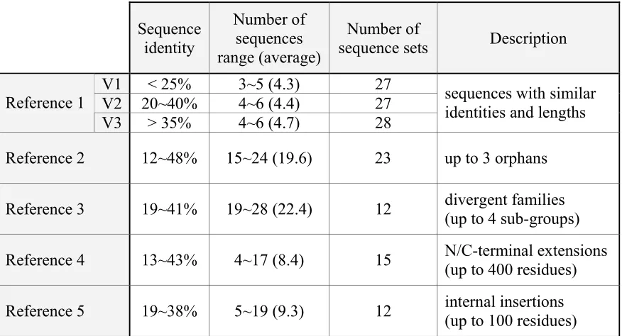
BAliBASE (benchmark alignment database) v1.0 provides 144 accurate reference alignments so that we can easily benchmark the performance of MSA methods. The sequence sets are categorized by length and sequence identity (%), compositional divergence, and the presence of orphan sequences (a sequence that has lower than 25% sequence identity with other members in a set), internal insertions, and N/C-terminal extensions (insertion of sub-sequence at the beginning or at the end of original sub-sequences). The core blocks (or conserved regions) in a sequence set are capitalized and marked with underlines so that we can see whether a test MSA method can catch biologically significant signals of residue

equivalencies.

Table 2.1: The description of BAliBASE categories

Sequence identity

Number of sequences range (average)

Number of

sequence sets Description V1 < 25% 3~5 (4.3) 27

V2 20~40% 4~6 (4.4) 27

Reference 1

V3 > 35% 4~6 (4.7) 28

sequences with similar identities and lengths

Reference 2 12~48% 15~24 (19.6) 23 up to 3 orphans

Reference 3 19~41% 19~28 (22.4) 12 divergent families _{(up to 4 sub-groups)}

Reference 4 13~43% 4~17 (8.4) 15 N/C-terminal extensions_{(up to 400 residues)}

(25)

BAliBASE also provides a standard program, BaliScore, that evaluates accuracies of the MSA results. The program computes two different scores for each alignment: one is sum-of-pairs score (or SP score) that estimates the ability to identify correct residue pairs, and the other is column score (or TC score) that assess the competence in correctly aligning the entire column. The two scores are calculated by the following equations.

SP Score =

∑

= = Mr j j Mt i i

r

t

1 1 (2.2)

where ti =

∑∑

= =

N

u N

v

p

iuv 1 1

, rj =

∑∑

= =

N

u N

v

p

juv 1 1

each for test and reference alignment,

N is the number of sequences contained in the problem set Mt is the number of columns in test alignment, and

Mr is the number of columns in reference alignment.

TC Score =

M

c

t Mt i i

∑

=1 (2.3)

where ci =

u≠v u≠v

1 if residues Ru and Rv in the i-th column are aligned

0 otherwise, piuv =

(26)

The performance (SP scores only) of other well-known MSA methods are available in the website http://www-igbmc.u-strasbg.fr/BioInfo/BAliBASE/prog_scores.html [28]. But T-Coffee outperformed all the other methods on average, so, in this research, we will

(27)

CHAPTER 3

The Principles of P-Coffee

In this chapter we explain the operation of our approach, P-Coffee. Specifically, we show in detail how partition walls are identified from a given set of sequences, and how P-Coffee aligns sequences with identified walls. An illustrative example of identifying a partition wall is also given.

3.1 Identification of Partition Walls

(28)

3.1.1 The Definition of Partitions and Partition Walls

A partition wall is defined as a set of residues, each of which is chosen from the given sequences. At most one residue can be chosen from each sequence. If no residue is chosen from a sequence, a gap is used in its place. A partition wall exactly corresponds to a column in a candidate alignment solution for a given sequence set. A complete wall refers to one that does not contain any gaps. Two walls are compatible if they are completely

separated and do not cross over each other. Otherwise, two walls are said to be conflicting. The residues in a partition wall are sorted in the order of sequence id (usually a unique integer assigned to each sequence) so that we can easily check the compatibility of two walls.

A partition is a set of sub-sequences between two complete walls. A sub-sequence can be a null string if no residues of a certain sequence are involved in the partition. A partition cannot include any walls. The partitioning refers to dividing a given sequence set into multiple disjoint partitions sectioned by single or multiple partition walls.

(29)

share some sub-sequences, which will be divided when more walls become available in later steps. Note that virtual walls cannot be used to construct the entire alignment, because they do not exist in reality.

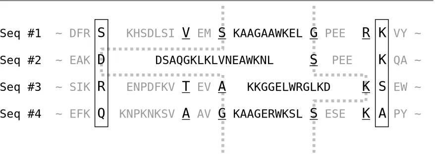
In the case illustrated in Figure 3.1, there are two complete walls {S, D, R, Q} and {K, K, S, A}, which are placed in solid boxes. There are four incomplete walls, which contain underlined residues: {V, −, T, A}, {S, −, A, G}, {G, S, −, S}, and {R, −, K, K}. Gaps are denoted by ‘−’. Walls are aligned because they correspond to the columns in some alignment, as mentioned earlier.

Figure 3.1: An example of virtual walls (sequences from 1aab_ref1 in BAliBASE v1.0)

Suppose we want the partition between the walls {S, −, A, G} and {G, S, −, S}. Because both of the walls are incomplete, we have to construct virtual walls to obtain the partition. In the left wall {S, −, A, G}, the gap for sequence #2 should be replaced with the residue in the nearest left wall with no gap for sequence #2. In this case, because {V, −, T, A} had again a

Seq #1 ~ DFR

S

Seq #2 ~ EAK

D

Seq #3 ~ SIK

R

Seq #4 ~ EFK

Q

R K VY ~

K QA ~

K S EW ~

K A PY ~

KHSDLSI

V

EM

S

KAAGAAWKEL

G

PEE

DSAQGKLKLVNEAWKNL

S

PEE

ENPDFKV

T

EV

A

KKGGELWRGLKD

(30)

gap for sequence #2, we had to borrow a residue from {S, D, R, Q}, one of the complete walls. Thus the left virtual wall is {S, D, A, G}. Similarly, for the gap in the right wall {G, S,

−, S}, we fill the gap for sequence #3 with the residue in the nearest right wall {R, −, K, K}. Note that {R, −, K, K} is not complete, but holds a residue for sequence #3. Thus the right virtual wall is {G, S, K, S}. The resulting partition is, therefore, {KAAGAAWKEL, DSAQGKLKLVNEAWKNL, KKGGELWRGLKD, KAAGERWKSL}.

3.1.2 The Advantages of Partitioning

Partitioning a set of sequences at hand has two major advantages.

First, it reduces the individual problem size by dividing the original sequence set into multiple independent sets of sub-sequences. Once a partition is fixed, we do not need to consider alignment between a residue inside the partition and others outside the partition. This significantly reduces the complexity in aligning the sub-sequences in a certain partition, when compared with aligning without partitioning. The most important point here is that the problem complexity reduces to O(L), linear time in the (average) length of the sequences, assuming the number of sequences is fixed. Some partitions will contain null strings as partitioning advances. For these partitions, we are only concerned with the remaining sequences. Because the running time of the depth-first tree search algorithm is O(Bd), where B is the branching factor and d is depth, the reduced depth of the problem will also result in considerable speedup. We can obtain the overall alignment solution by simply

“concatenating” the alignment of each partition and partition walls in the original order provided in the sequence set.

(31)

qualified partition walls during the running of the algorithm. As mentioned in the previous section, a partition wall corresponds to a column in the alignment solution. Thus, to reach an alignment solution, we can pay our attention only to unaligned portions, which are partitions.

3.1.3 Steps to Identify a Partition Wall

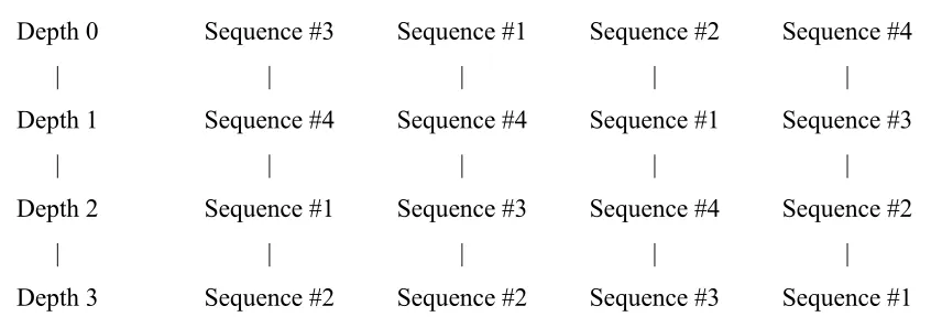
Step 1.Generate a random hierarchy

As mentioned in Chapter 2, T-Coffee aligns sequences using a progressive approach that relies on multiple running of dynamic programming in the order implied by a

precomputed phylogenetic tree. Instead of depending upon such a “hypothetical” tree, P-Coffee generates a random hierarchy, which defines the contingent rank of each sequence. This hierarchy is used when P-Coffee constructs a tree, and coordinates the parent-child relationship among residues. Some of possible random hierarchies are shown in Figure 3.2. In this four-sequence case, there exist 4! = 24 different hierarchies.

(32)

Step 2.Build a tree beginning with a residue randomly picked from the depth-0 sequence

Given a random hierarchy, P-Coffee starts building a tree by choosing one residue from the depth-0 sequence. Beginning with the chosen residue as the root of the tree being constructed, P-Coffee recursively attaches the residues that are contained in the T-Coffee library when paired with the current parent residue. The simple rule here is that residues in depth-(i) are rendered to be parent nodes of ones in depth-(i+1). In other words, edges are directed in increasing order of depth, from lesser to greater. A tree is built in depth-first fashion, and, when there are no residues that can be added to the current node, the tree extension can stop even before it reaches the maximum depth.

Step 3.Do the depth-first search for the highest-scored path in the fully-grown tree

(33)

3.2 Techniques to Speedup the Wall Identification Process

In order to speedup the identification process of partition walls, we use several tricks during the tree construction procedure. The tricks used here are not new, but helpful in making this recursive procedure affordable.

3.2.1 Combination of Tree Building and the Highest Scorer Searching

Because trees are needed only to obtain the highest-scored path, we can speed up the identification process by combining the tree construction and the highest-scored path search. Specifically, we update the position of current highest-scorer as well as its score whenever a node is added to the tree. In this way, we get the highest-scored path as soon as we finish constructing a tree. Trees are discarded without being stored in order to save memory.

3.2.2 Thresholding

Even if a residue found as a child lies within a partition range, we may not want to add it because we regard the entailed pair score to be unreliable and presumably safely neglected. The objective of thresholding is “not” to add a node that is expected to be

unreliable as a member of a path being extended. But of course, if the threshold pair score is set too high, the algorithm will branch away from a node that is required to successfully construct a wall with maximum available reliability.

(34)

consistency of each residue pair. Therefore, sequence identity is the minimum score that is guaranteed to any aligned residue pairs in T-Coffee extended library. In addition, it is reported that sequence comparison detects relationships between protein residues reliably down to about 30% sequence identity [5]. For all these reasons, it is expected that the appropriate threshold score can be determined near the range of “twilight zone” identities.

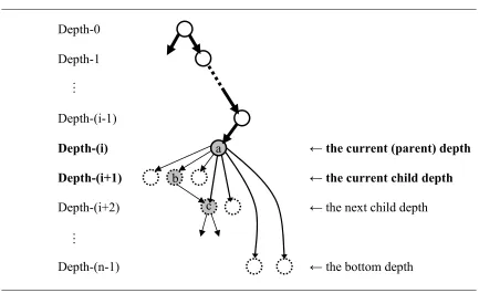
Under the sum-of-pairs scoring scheme, one additional child node brings in multiple pair scores. As shown in Figure 3.3 by the bold bi-directional arrows, we consider all possible pairs between the child node at hand and the predecessor nodes in the path being constructed.

Figure 3.3: The number of new residue pairs generated by adding a child Depth-0

Depth-1

Depth-(i-1)

Depth-(i)

Depth-(i+1)

Depth-(i+2)

… …

The path that is currently being extended

← the current (parent) depth

← the current child depth

← the next child depth

…

(35)

We apply a threshold pair score to the average of all the pair scores generated by adding a child node. In this way, a child node that has fewer but stronger connections with its predecessors can also be accepted.

3.2.3 Pruning

We can further save resources (computation time and memory) by “not” adding a child if no relevant future path can possibly outscore the current highest. The maximum substitution score can be trivially found in the T-Coffee extended library. And, we also know the remaining depths to go and, therefore, the maximum number of residue pairs that will be brought in under the sum-of-pairs scoring scheme. Therefore, by giving each residue pair the maximum substitution score in the T-Coffee library, we can easily compute the upper bound on the score that can be achieved by the path that is currently being extended. By comparing this estimated upper bound with the current highest that is previously found, we can decide whether to add a child node or not.

3.2.4 Sorting of Candidate Child Nodes

To maximize the effectiveness of pruning, it is better to come up with as high as possible a score in earlier stage of the tree construction. To promote this situation, we designed our method to consider pairs in decreasing order of score when examining

(36)

3.2.5 Jumping

Jumping describes finding related residues from lower depths than the current child depth. Since with jumping more candidate residues are within the scope of a parent node, this modification considerably increases the average branching factor. Thus, more candidate paths (partition walls) are examined while searching for the highest-scored path. There is a trade-off between the thoroughness of searching and the resulting computational cost.

Although a more branched tree would result, jumping does not mean that we can necessarily identify a more reliable path from the tree, because of a side effect incurred by jumping: jumping introduces a gap for the skipped sequence. For example, the one step jumping from node (a) to node (c) will result in the path {…, a, −, c, …} as shown in Figure 3.4.

Figure 3.4: Jumping Depth-0

Depth-1

Depth-(i-1)

Depth-(i)

Depth-(i+1)

Depth-(i+2)

Depth-(n-1)

……

← the current (parent) depth

← the current child depth

← the next child depth

← the bottom depth c

(37)

Dotted circles denote candidate nodes that may be added to the current (parent) node, which is currently the node (a). Since a gap significantly reduces the sum-of-pairs score of a wall by negating maximum (n – 1) substitution scores, where n denotes the total number of sequences, a path with jumping history is less likely to make the highest score in the tree. This can be easily noticed by comparing the score of the path {…, a, b, c, …} with that of the path {…, a, −, c, …}. The latter will lose every pair score that involves the node (b), under the sum-of-pairs scoring scheme.

(38)

3.3 Example of Identifying a Partition Wall

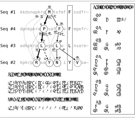
Figure 3.5 shows the 1aab (reference 1) case given in BAliBASE v1.0. Suppose a random hierarchy #1→ #4→ #3→#2 is generated, and 1-11 (residue #11 of sequence #1) is randomly picked as the root of the tree that is going to be constructed.

Figure 3.5: An example of tree construction. The path {F, F, L, Y} in a solid block denotes a previously identified complete wall, by which a partition is formed on its left side. Jumping is not allowed. The terms in the sum-of-pairs scores are given in the order of (1,4), (1,3), (1,2), (4,3), (4,2), and (3,2), where (i, j) denotes the pair of sequence id’s. The table of substitution scores is given as is in T-Coffee extended library.

kkdsnapkra M tsfmf F ssdfr~

dpnkpkra P saf F v F mgefr~

adkpkrp L aym L w L nsare~

kpkrp R sa Y N i Y V sa~

Seq #1

Seq #4

Seq #3

Seq #2

11 9 87 99 87 8 10 107 20 13 9 25 12 13 107 87 20

Related residue pair scores # 1 2

11 6 99 (*)

# 1 3

11 8 65

# 1 4

11 9 105

11 13 25

# 2 3

6 8 87

9 8 20

10 12 87

13 12 20

# 2 4

6 9 87

9 9 27

10 13 87

# 3 4

8 9 107

12 13 107

The sum-of-pairs score of each path

{M, P, L, R}: 105 + 65 + 99 + 107 + 87 + 87 = 550 {M, P, L, Y}: 105 + 65 + 0 + 107 + 27 + 20 = 324 {M, F, L, N}: 25 + 0 + 0 + 107 + 87 + 87 = 306 An example score calculation of a jumping path {M, P, –, Y}: 105 + 0 + 0 + 0 + 27 + 0 = 132

27 105 65

6

(39)

The relevant residue number is put on the top of each node. And, the substitution scores are placed at the bottom of each node, near the starting point of each directed edge. The relevant substitution scores are excerpted from the T-Coffee extended library that is computed beforehand for this sequence set. The lines with # sign specify the sequence numbers. Other lines indicate residue pair by their position indices in each sequence, and its score (bold face). For example, the line marked (*) means that the substitution score between 1-11 and 2-6 is 99.

A tree is built starting from the randomly picked root 1-11. So the current ongoing path is {1-11}. By the random hierarchy, sequence #4 is at the current child depth. So we refer to the category [# 1 4] in the T-Coffee library, and find out that 1-11 is related to 4-9 and 4-13, whose scores are 105 and 25 respectively. Because 4-9 makes higher score with 1-11, it is first checked for attachment. Suppose we set the threshold pair score to 10. Because the average score between 4-9 and every node in the ongoing path {1-11} is 107 / 1 = 107 > 10, it clears threshold condition. Next we check the pruning condition. From the current child depth, there are two more depths to go, so maximum 2 + 3 = 5 residue pairs would be

brought in until the path reaches to the bottom depth. Because the maximum pair score is found to be 107 for this set, the upper bound score the path {1-11, 4-9} can achieve is 107 + 107 × 5 = 642. This outscores the current highest, which is zero. So the candidate 4-9 also clears the pruning condition, thus it is added to the root 1-11. The current ongoing path becomes {1-11, 4-9}. The current highest is reset to node 4-9 with the score of 107.

(40)

According to the score, the path {M, P, L, R} is the highest-scored path. By sorting the nodes in the path in the order of sequence id, the partition wall {M, R, L, P} is obtained.

(41)

3.4 Partition Wall Selection for Alignment Solution Construction

The reliability of an alignment solution depends upon that of columns used to

construct the alignment. Since columns correspond to partition walls in P-Coffee, it is crucial to correctly evaluate the reliability of the walls found during the wall identification procedure. In this section, we propose an additional criterion other than the sum-of-pairs score to select reliable walls from the pool of identified walls.

3.4.1 Reliability of a Partition Wall

There are some issues about the reliability of partition walls. What is the reliability of a partition wall, and how can we evaluate it? Does a higher sum-of-pairs score mean a more reliable partition wall? Is the score the only criterion for reliability we can depend upon?

As for reliability, we can simply state that reliable walls should be able to catch biologically meaningful residue equivalency. In fact, discovering correct residue

equivalencies from given protein sequences is the essence of all sequence alignment tools, in that structure or function of proteins are predicted based on these equivalencies. On the other hand, evaluating residue equivalency is not as straightforward as the objective itself, because of the lack of dependable arrangements to incorporate information that relates residues into sequence-level analysis. There have been efforts to exploit other source of equivalency information such as structural data [29]. But, coming up with a sound objective function to evaluate residue equivalencies is still an important issue.

(42)

in the reference alignment. We found that walls falling in only upper 15% of score range can be used safely to construct alignment solutions.

Facing this challenge, we paid an attention to an important point: the sum-of-pairs scoring scheme reflects the interrelatedness among residues contained in a column (or a wall). Based on the idea, we invented a test that detects more reliable walls from the pool of identified walls.

3.4.2 The True Power of Random Hierarchy

The breakthrough for the difficulty in reliability evaluation is to accept walls that appear more than some specified number of times after a sufficiently large number of iterations of wall identification. As explained in Section 3.1.3, P-Coffee first generates a random hierarchy, and arbitrarily chooses one residue from the depth-0 sequence as root to be extended. In each iteration, a different sequence hierarchy as well as a root is used, and extended fully to a different tree. During this iterative procedure, a certain wall may be identified more than once if residues contained in the wall are closely interrelated. Therefore, by accepting reproducible walls, we can mimic the idea of the sum-of-pairs scoring scheme. The advantage of this test is that it does not depend upon any scoring metric, so even

relatively low scorers may be accepted.

(43)

hypothetical phylogenetic trees but also to provide a novel way to discover the interrelatedness among residues.

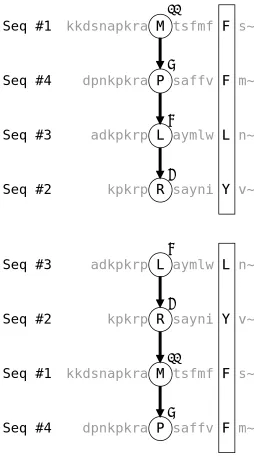
This can be illustrated by comparing Figure 3.5 and Figure 3.6. It can easily be noticed by directed edges that the residues in the highest-scored path {M, P, L, R} are

interrelated in Figure 3.5. In Figure 3.6, we use a different hierarchy #3→ #2→ #1→#4 and a different root 3-8, and found the different highest scored path {L, R, M, P}. But as indicated in Figure 3.7, these two paths imply the same wall, {M, R, L, P}.

Figure 3.6: Another random tree for the Section 3.3 example

a d k p k r p L aymlw L ns~

k p k r p R sa Y ni Y vs~

kkdsnapkra M ts F mf F ss~

dpnkpkra P sa F F v F M ~

Seq #3

Seq #2

Seq #1

Seq #4

11 9 99 87 8 12 105 14 9 25 16 13 25 ₁₀₅

Related residue pair scores # 1 2

11 6 99

14 9 99

# 1 3

11 8 65

67 8 28

# 1 4

11 9 105

11 13 25

14 12 105

14 16 25

# 2 3

6 8 87

9 8 20

# 2 4

6 9 87

9 9 27

# 3 4

8 9 107

The sum-of-pairs score of each path

{L, R, M, P}: 87 + 65 + 107 + 99 + 87 + 105 = 550 {L, R, M, F}: 87 + 65 + 0 + 99 + 0 + 25 = 276 {L, Y, F, F}: 20 + 0 + 0 + 99 + 0 + 105 = 224

20

6

99 107 65

(44)

Figure 3.7: The wall identified by two different random trees

kkdsnapkra M tsfmf F s~

dpnkpkra P saffv F m~

adkpkrp L aymlw L n~

kpkrp R sayni Y v~

Seq #1

Seq #4

Seq #3

Seq #2

11

9

8

6

adkpkrp L aymlw L n~

kpkrp R sayni Y v~

kkdsnapkra M tsfmf F s~

dpnkpkra P saffv F m~

Seq #3

Seq #2

Seq #1

Seq #4

8

6

11

(45)

3.4.3 The Construction Procedure of Alignment Solution

The target alignment is constructed by recursively partitioning the given sequence set. There are two base cases available for this recursive procedure. If a partition is composed of at most one residue for each sequence, P-Coffee fixes the partition as one partition wall. If a partition contains only residues that belong to a certain sequence, P-Coffee separates them into distinctive columns that contain only one residue. After all partitions are fixed, P-Coffee concatenates them into one big alignment solution. To save memory, we implemented this recursive procedure so as to keep only selected walls and to handle each partition between two walls one by one. Every partition from the leftmost one to the rightmost one undergoes further partitioning during one phase.

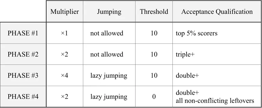
There are parameters to be determined before running P-Coffee. The threshold pair score is a parameter for screening out unreliable residues in order to speed up the wall identification process. The threshold score of 10 is used throughout the phases except the last one. The Multiplier is a parameter that defines the number of iterations for each phase. If it is “×2”, the wall identifying procedure is repeated twice the maximum sequence length number of times in the partition at hand. The Acceptance Qualification describes which walls to accept in each phase. If it is “double+”, we only accept walls that are identified more than once. We also have to decide whether to allow jumping. Detailed description of the parameters is given in the next section.

(46)

wall between them. Therefore, it is important to select more reliable walls in the earlier stages, so that partitions can safely disregard outsider residues during the iterative

partitioning process. Based on this idea, we designed P-Coffee to work in four phases. The values of the parameters are summarized in Table 3.1.

Table 3.1: Phases in P-Coffee. Jumping is not a parameter for the algorithm, but included in this table to show when it is activated. In phase #4, the acceptance qualification gives the priority in the order of double+’s, and then, the high scorers.

Multiplier Jumping Threshold Acceptance Qualification

PHASE #1 ×1 not allowed 10 top 5% scorers

PHASE #2 ×2 not allowed 10 triple+

PHASE #3 ×4 lazy jumping 10 double+

PHASE #4 ×2 lazy jumping 0 double+ _{all non-conflicting leftovers}

(47)

portion of all identified walls. The wall identification is repeated the maximum sequence length number of times. The reproducibility criterion is not applied in this phase.

In Phase #2, P-Coffee repeats the wall identification process for ×2 times to find more walls that are reproducible. Only walls that identified more than twice are accepted. In Table 3.1, these walls are denoted by “triple+”, meaning the walls that appear “three times or more” in one phase. The acceptance qualification is set to triple+ in order to select more reliable walls in the earlier stages. Jumping is not allowed, because we expect that there still remain many undiscovered complete walls since only 5% of walls are fixed in the previous phase. Note that scores are not used for acceptance checking.

In Phase #3, lazy jumping is allowed so as to effectively identify walls that contain gaps. Complete walls may still remain. But, if this is the case, lazy jumping will not actually be used, since it is called only when there is no candidate child to be added at the current child depth. To find more reproducible walls, we raise the multiplier to ×4. Walls identified more than once are accepted. We denote these walls “double+” to represent the ones that appear “two times or more” in one phase. No scores are used for acceptance either in this phase.

(48)

3.5 Parameters

There are four parameters that have to be set before running P-Coffee. The threshold pair score is required for efficient running of the wall identification process. The multiplier and the acceptance qualification including the initial acceptance rate control the wall selection procedure. In this section, we will describe in detail the features that these parameters have.

3.5.1 The Threshold Pair Scores

As explained in Chapter 2, sequence identity (%) is the minimum score that is guaranteed to the aligned residue pairs belonging to the sequences. Admitting that sequence comparison is reliable down to the twilight zone (25~30% identity), we may conclude that we can ignore residue pairs with substitution score below this zone when extending a tree. But if multiple sequences are used in search of hidden residue equivalencies, interrelatedness among residues may be helpful in identifying reliable equivalencies below this limit. More importantly, it is impossible to construct an alignment solution with columns that are

composed of only reliable residues, because in MSA we have to assign every residue to some position in the alignment, irrespective of its reliability. Therefore, in the big picture, we cannot ignore residues just because they entail substitution scores below the twilight zone.

Because of the lack of information sufficient to overcome this complexity, we decided the proper level of the threshold pair score experimentally by observing the effect of threshold values on algorithm performance.

(49)

amount of computational resources. Note that this tree-based procedure has exponential time complexity, so controlling the branch factor is crucial. On the other hand, if we set the threshold excessively high, it will prevent the paths being constructed from reaching to the bottom depth without gaps, thus making them unlikely to survive the competition among paths in the tree. We want to find the optimum threshold value that controls the exponential time complexity without sacrificing the reliability of identified walls.

3.5.2 The Multiplier and The Acceptance Qualification

As described in Section 3.4.3, the multiplier specifies the number of iterations used to form a pool of partition walls in each phase, and the acceptance qualification describes a condition for the walls to be accepted. We use the maximum sequence length as a multiplicand so that each residue in the maximum length sequence can be examined

probabilistically at least once. Note that the closest number to the resulting alignment length currently available is the maximum sequence length, because no two residues in the same sequence can be in the same alignment column.

(50)

number of qualified walls will be reduced, since walls do not have enough chance to appeal their reliability.

3.5.3 The Initial Acceptance Rate

The initial acceptancerate is one of the acceptance qualifications that is used only in the initial phase of P-Coffee. The motivation of using the initial acceptance rate is that there may exist a minimum score that we can use as a cutoff criterion when selecting a wall from the pool of identified walls. Since this minimum will be different case by case, we normalize it by the highest score found during the repetition of wall identification process.

The initial acceptance rate is defined by the following formula. So, for example, if the rate is set to 10%, we will accept only the top 10% highest scorers from the identified walls in Phase #1.

the initial acceptance rate = 1 − normalizedminimum score for guaranteed hit score

highest overall

the

score fail highest the

−

= 1 (3.1)

(51)

CHAPTER 4

Tests and Results

In the previous chapter, we explained some features that are introduced for more effective and accurate running of the algorithm. We pointed out four parameters to be determined before the running of P-Coffee. In this chapter, we will demonstrate how the parameters have been determined. And then, we will show the competency of P-Coffee by comparing its performance with T-Coffee using BAliBASE v1.0 test cases.

4.1 Tests

(52)

4.1.1 Test #1: The Optimum Threshold Pair Score

One of the most important benefits of BAliBASE is that we can evaluate the correctness of an identified wall by simply seeing whether it is really included in the

reference alignment or not. We call it a hit if we can find a match, and a fail otherwise. Using this feature, we can obtain the hit rate of the identified walls after repeating the wall

identification process for a specified number of times. In this test, we want to know to what extent the algorithm should allow unreliable (lower scored pair) residues to be added to a tree being constructed. So we can find out the optimum threshold value by selecting one that makes the maximum hit rate. We tested 5, 10, 15, and 20 as the threshold values with the multiplier value of ×1. We did not allow jumping in this test.

4.1.2 Test #2: The Optimum Initial Acceptance Rate

In this test, we wanted to find out the maximum level of acceptance rate that would cover most of the test cases. This test can be done alongside Test #1, since we can obtain the initial acceptance rate of each test case by simply keeping track of the highest fail score and the overall highest during the iteration.

4.1.3 Test #3: The Optimum Combination of the Multiplier and the

Acceptance Qualification

(53)

We tested the multiplier values of ×1, ×2, ×3, and ×4, and analyzed the hit rate as well as the number of identified walls for the qualification values of singles, double+’s, and triple+’s for each multiplier value. We used the threshold pair score of 10, and did not allow jumping in this test.

4.1.4 Test #4: The Performance of P-Coffee

BAliBASE also provides a program, BaliScore, so that we can score our results according to the standardized guideline. This score can be used to benchmark the

(54)

4.2 Test

Results

4.2.1 The Optimum Threshold Pair Score

As expected, if the threshold pair score is smaller, an exponentially larger amount of CPU time is used to identify partition walls, because the branch factor of trees will increase. The result is shown in Table 4.1 and Figure 4.1. But lower thresholds did not always result in higher hit rates. This means that a branchy tree does not guarantee finding more reliable partition walls. Rather, in many cases, hit rates decreased with the threshold values lower than the optimums, because it is more likely that unnecessary residues are included in the surviving walls.

Table 4.1: The performance of the partition wall identification with the varying threshold pair scores. 1idy (ref 2), 1lvl (ref2), 1tgxA (ref2), and 1idy (ref3) are excluded from this result to avoid a bias that can be arise as a result of their excessive amount of CPU time (in seconds) used.

Threshold = 5 Threshold = 10 Threshold = 15 Threshold = 20 Hit

Rate

CPU Time

Hit Rate

CPU Time

Hit Rate

CPU Time

Hit Rate

CPU Time

Ref 1 0.819 47 0.828 53 0.793 35 0.747 42

Ref 2 0.542 15200 0.542 5043 0.400 1141 0.305 811

Ref 3 0.541 18242 0.565 1265 0.423 227 0.317 157

Ref 4 0.575 425 0.519 211 0.469 92 0.383 88

Ref 5 0.730 576 0.731 216 0.726 96 0.692 95

(55)

0.000 0.100 0.200 0.300 0.400 0.500 0.600 0.700 0.800 0.900 1.000

5 10 15 20

The Threshold Pair Score

Hi t Ra te 0 500 1000 1500 2000 2500 3000 3500 4000 C P U T im e (s ec onds ) Ref1 Ref2 Ref3 Ref4 Ref5 Avg Hit Rate Avg CPU Time

Figure 4.1: Effect of the threshold pair score on the performance of the wall identification process. The average hit rate declines from the threshold value of 10.

(56)

4.2.2 The Optimum Initial Acceptance Rate

For each threshold value that was used in the previous test, the initial acceptance rates were observed. The result is summarized in Table 4.2. For example, the cell that is marked (*) in Table 4.2 means that only the top 3.9% of the highest scoring walls were correct in Reference 2 test cases when we use the threshold value of 10. Walls with scores below that level are no longer safe to use to construct alignment solutions without further analysis.

The rates turn out to be insensitive to the threshold values. This is because the highest fail score and the overall highest could be found no matter what threshold value below the twilight zone is used.

Table 4.2: Reliable score range of sum-of-pairs scoring scheme

Threshold 5 10 15 20

Ref 1 0.209 0.207 0.210 0.200

Ref 2 0.039 (*) 0.039 0.039 0.041

Ref 3 0.071 0.070 0.063 0.066

Ref 4 0.092 0.086 0.087 0.089

Ref 5 0.199 0.137 0.140 0.135

(57)

The data shows that, on average, only the top 15% highest scorers were reliable under the sum-of-pairs scoring scheme. But, considering the narrowest range among all categories (see the cell marked (*) in Table 4.2), we decided to accept only the top 5% highest scorers in the first phase of P-Coffee. Figure 4.2 illustrates how many categories the optimum initial acceptance rate covers.

0.000 0.050 0.100 0.150 0.200 0.250

Ref1 Ref2 Ref3 Ref4 Ref5 OVERALL

BAliBASE Categories T he Low e s t F a il S c o re / T h e M a x im u m S c or e

Threshold = 5 Threshold = 10 Threshold = 15 Threshold = 20

Figure 4.2: The reliable range of the sum-of-pair scores Reference 2 has the

(58)

The selected initial acceptance rate does not fully cover the test cases in Reference 2. But even incorrect walls with scores near this region will not harm the reliability of an overall alignment solution, since they would not have reached such high scores without containing enough of the residue equivalencies we are looking for.

4.2.3 The Optimum Combination of Multiplier-Qualification

(59)

Table 4.3: The reliability of reproducible walls in various combinations of multiplier-qualification. The test cases, 1idy, 1lvl, and 1tgxA (all in reference 2), are excluded from this result. Because we counted the walls that are identified more than three times as three, the raw hit rates are estimated slightly lower than the real values.

Qualification Singles

Multipliers ×1 ×2 ×3 ×4

Ref1 0.681 0.479 0.304 0.176

Ref2 0.338 0.186 0.100 0.057

Ref3 0.345 0.177 0.090 0.050

Ref4 0.232 0.154 0.169 0.111

Ref5 0.510 0.275 0.156 0.097

Overall 0.497 0.298 0.190 0.110

Num of Walls 11272 9137 6861 4783

Qualification Double+

Ref1 0.945 0.928 0.905 0.879

Ref2 0.895 0.856 0.844 0.830

Ref3 0.988 0.979 0.968 0.961

Ref4 0.826 0.757 0.660 0.593

Ref5 0.948 0.942 0.923 0.903

Overall 0.928 0.907 0.878 0.848

Num of Walls 8115 17473 23186 26545

Qualification Triple+

Ref1 0.966 0.961 0.961 0.950

Ref2 0.919 0.911 0.901 0.894

Ref3 0.987 0.993 0.987 0.984

Ref4 0.925 0.908 (*) 0.841 0.802

Ref5 0.959 0.978 0.965 0.962

Overall 0.954 0.953 0.946 0.934

Num of Walls 2732 9767 16794 21840

Raw (estimated)

(60)

0.000 0.100 0.200 0.300 0.400 0.500 0.600 0.700 0.800 0.900 1.000

Ref1 Ref2 Ref3 Ref4 Ref5

BAliBASE Categories

Hit Rate

x1- Singles

x2- Singles

x3- Singles

x4- Singles

x1- double+

x2- double+

x3- double+

x4- double+

x1- Triple+

x2- Triple+

x3- Triple+

x4- Triple+

(61)

The overall average accuracy of each qualification is illustrated in Figure 4.4.

Compared with the raw accuracy, the selected combination achieved an accuracy increase of (0.953 – 0.602) / 0.602 ≈ 58%. Note that the limit we could have achieve was (1 – 0.602) / 0.602 ≈ 66%. Since over 95% of walls identified in Phase #2 are hits, this will significantly contribute to the reliability of overall alignment solution.

0.000 0.100 0.200 0.300 0.400 0.500 0.600 0.700 0.800 0.900 1.000

x1 x2 x3 x4

Multiplier

Hi

t Ra

te

Singles Double+ Triple+ Raw

(62)

The numbers of correct walls that are identified during the tests are illustrated in Figure 4.5. As mentioned in Section 3.5.2, the number of singles decreased as the multiplier was set to a larger value. Instead, more double+’s and triple+’s could be identified.

0 5000 10000 15000 20000 25000 30000

x1 x2 x3 x4

Multiplier

The Number of Correct Walls

Singles Double+ Triple+

Figure 4.5: The number of correct walls identified

(63)

(64)

4.2.4 The Performance of P-Coffee

The competency of P-Coffee is demonstrated by comparing its performance with that of Coffee. The differences between the percent accuracy achieved by P-Coffee and T-Coffee are plotted along with the average sequence identity of test sets. Both the residue pair accuracy and the column accuracy are compared, and each result is drawn separately as in Figure 4.6 (a) and (b). To make the differences clearer, we divided the data into two parts, Reference 1 and the others. As shown in Figure 4.7, we could not identify any improvement for the test cases in Reference 1. But, for References 2 to 5, which are composed of problem sets with more sequences, P-Coffee improved both the residue pair accuracy and the column accuracy on average by 6% and 18% respectively. As validated by the P-values for the Wilcoxon signed rank tests both less than 10-7_{, the difference between P-Coffee and T-Coffee}

is significant. This improvement can also be easily noticed by the dispersion of data points shifted towards upper region of x-axis in Figure 4.8.

Table 4.4: The average accuracy P-Coffee compared with that of T-Coffee.

SP Score TC Score

T-Coffee P-Coffee T-Coffee P-Coffee

Ref 1 94.1% 93.8% 89.3% 89.9%

Ref 2 86.6% 93.1% 35.5% 59.6%

Ref 3 92.2% 97.5% 62.9% 85.0%

Ref 4 78.5% 85.5% 57.0% 70.2%

Ref 5 93.7% 97.5% 82.8% 90.8%

Overall 91.1% 93.5% 74.6% 82.7%

(65)

-40% -20% 0% 20% 40%

0 20 40 60 80

Average % Identity

P -C o ff ee - T -C o ff ee (% A c c u ra c y ) -120% -100% -80% -60% -40% -20% 0% 20% 40% 60% 80% 100% 120%

0 20 40 60 80

Average % Identity

(66)

-40% -20% 0% 20% 40%

0 20 40 60 80

Average % Identity

0 20 40 60 80

Average % Identity

P -C o ff ee - T -C o ff ee (% A c c u ra c y )

Figure 4.7: The difference in (a) SP Score and (b) TP Score (Ref1 Only)

)

(a)

(67)

-40% -20% 0% 20% 40%

0 20 40 60

Average % Identity

0 20 40 60

Average % Identity

(68)

4.2.5 Further Analysis of the Performance of P-Coffee

P-Coffee outperformed T-Coffee in References 2 to 5 test cases. These categories contain 15.5 sequences on average, while Reference 1 contains only 4.5 sequences. If the number of sequences increases, the length of partition walls also increases. As a result, the probability that a certain wall is identified more than once gets smaller, since more residues should be interrelated. This makes the reproducible walls more reliable than those in cases with fewer number of sequences. As shown in Figure 4.9, the hit rates of both double+’s and triple+’s are distributed in the higher value range as the number of sequences increases.

0.000 1.000

0 5 10 15 20 25 30

The number of sequence

H

it r

a

te

Double+

Triple+

(69)

4.2.6 The Run Time Analysis of P-Coffee algorithm

We analyzed the run time of P-Coffee with a fixed number of sequences, in order to prove the advantage of partitioning. If the number of sequences is fixed, the run time of the algorithm is expected to be O(L), where L is the average length of the sequences, because the number of partition walls to be identified will increase proportional to the average length of the sequence set in most cases. The analysis was done only with Reference 1 test cases, because it is the only category that has enough data points that share the same number of sequences. As illustrated in Figure 4.10 and Figure 4.11, the CPU time increased linearly in the length of the sequence set.

-100.0 0.0 100.0 200.0 300.0 400.0 500.0 600.0

0 200 400 600 800 1000 1200

The Alignment Length

CPU Time (seconds)

ref1 v1 ref1 v2 ref1 v3 ref4

Linear (ref1 v2)

(70)

-100.0 0.0 100.0 200.0 300.0 400.0 500.0 600.0

0 100 200 300 400 500 600 700 800 900

The Alignment Length

CPU T

ime (s

ec

onds

)

ref1 v1 ref1 v2 ref1 v3 ref4 ref5

Linear (ref1 v3)

Figure 4.11: Run time analysis of P-Coffee with a fixed number of sequences (5-sequence cases). The trend line in each graph of Figure 4.10 and Figure 4.11 is drawn only for the sub-category that has the maximum range in the sequence length. We used the length of the reference alignment instead of the average sequence length in this graph.

(71)

guarantee to hold an arbitrary sequence sets within the linear time complexity, as suggested by the outlier.

0.0 500.0 1000.0 1500.0 2000.0 2500.0 3000.0 3500.0

0 5 10 15 20

The number of Sequences

CPU Time (seconds)

ref4 ref5 Linear (ref5)

Figure 4.12: Run time analysis with varying number of sequences (Ref 4 and 5 only). A trend line is added for reference 5 cases.

(72)

T-environmental factors can be augmented. For this reason, it was difficult to analyze the influence of the techniques for speedup. This is well illustrated in Figure 4.13 by the widespread dispersion of data points. That is, for References 2 and 3 categories, it was not possible to identify any trend in the run time with varying number of sequences.

0 10000 20000 30000 40000 50000 60000 70000 80000

15 17 19 21 23 25 27 29

The Number of Sequences

CPU Times of Ref 2 (seconds)

0 1000 2000 3000 4000 5000 6000 ref2 ref3

Figure 4.13: Run time analysis with varying number of sequences (Ref 2 and 3 only)

CPU

Time

s

o

f Ref 3 (se

P-Coffee: A New Divide-and-conquer Method for Multiple Sequence Alignment

ABSTRACT

P-Coffee: a new divide-and-conquer method

for multiple sequence alignment

DEDICATION

BIOGRAPHY

ACKNOWLEDGMENTS

TABLE OF CONTENTS

LIST OF FIGURES

LIST OF TABLES

CHAPTER 1

Introduction

1.1

Cells and Proteins

1.2

Evolution from the Standpoint of Molecular Level

1.3

Phylogenetic Relationship among Proteins

1.4

The Importance of Sequence Alignment Methods

1.5

Multiple Sequence Alignment

1.6

Our Approach

1.7

Outline

CHAPTER 2

Background Information

2.1

Optimization Algorithms

2.1.1

Progressive Methods

2.1.2

Iterative Methods

2.2

Objective Functions

2.2.1

PAM Matrices

2.2.2

BLOSUM Matrices

2.2.3

Consistency-based Objective Function

∑

∑∑

2.3

BAliBASE

∑

∑

r

t

∑∑

p

∑∑

p

M

c

∑

CHAPTER 3

The Principles of P-Coffee

3.1

Identification of Partition Walls

3.1.1

The Definition of Partitions and Partition Walls

S

D

R

Q

R K VY ~

K QA ~

K S EW ~

K A PY ~

V

S

G

S

T

A

3.1.2

The Advantages of Partitioning

3.1.3