ABSTRACT
YI, SHENG. Shape Dynamic Analysis. (Under the direction of Dr. Hamid Krim.)
Shape has already been a critical feature to many vision applications like object detec-tion, contour tracking and activity recognition. In contrast to singularity based features like edge or texture, a shape is a structured feature with a more explicit geometric defi-nition. The mathematical elegance of shape representation brings in a lot of theoretical analysis of shape space, for instance, the metric, the geodesic path and the statistic in shape space. These theoretical results provide a fundamental support for shape based applications.
Most of the previous shape analyses focused on the point-wise geometry in a shape space, for example, the distance between two arbitrary shapes. However, only a few works elaborated on the dynamics in shape space. In this dissertation, we address the problem of shape dynamics analysis through different levels: (1) the bottom level segmentation in an image; (2) the middle level shape tracking, dimension reduction; and (3) the high level shape dynamic modeling, recognition.
c
Copyright 2011 by Sheng Yi
Shape Dynamic Analysis
by Sheng Yi
A dissertation submitted to the Graduate Faculty of North Carolina State University
in partial fulfillment of the requirements for the Degree of
Doctor of Philosophy
Electrical Engineering
Raleigh, North Carolina
2011
APPROVED BY:
Dr. Larry K. Norris Dr. Michael B. Steer
Dr. Griff L. Bilbro Dr. Hamid Krim
DEDICATION
BIOGRAPHY
ACKNOWLEDGEMENTS
I am very lucky in my PhD studies. I received a lot of help from many great people. First I would like to thank my adviser Dr. Hamid Krim for his insightful advise and invaluable support for my crazy ideas. His stimulating suggestions and ideas, continued mentoring and encouragement made my research really enjoyable. I also want to thank my committees, Dr. Michael Steer, Dr. Griff Bilbro, Dr. Larry Norris and Dr. Demetrio Labate for their support and comments to my research.
Particularly, I am greatly thankful to Dr. Demetrio Labate and Dr. Larry K. Norris, whose enlightening mathematical advice and education is invaluable for my research.
I am also very grateful to my lab-mates, Shuo Feng, Alex Chen, Aouada Djamila, Deokwoo Lee, Tian Wang, Scott Clouse, Xiao Bian, Sun Miao, Harish Cintacunta, Jen-nifer Gamble and Lu Han. The time we spent together were so happy and meaningful. I believe, one day, the dreams we shared will come true. I am very lucky to have met all of you in my life at NCSU.
Reviewing the very beginning of my research, I want to thank Dr. Xutao Li. Your talent, passion and belief in the signal and image processing have motivated me ever since 2005. The research integrity you are hold is always a reference for my own.
I want to thank my parents for your love support for all my life. I won’t have all of these without you.
TABLE OF CONTENTS
List of Tables . . . vii
List of Figures . . . viii
Chapter 1 Introduction . . . 1
1.1 Motivation . . . 1
1.2 Organization and Publications . . . 3
Chapter 2 Background . . . 6
2.1 Review of Wavelet Framework for Image Analysis . . . 6
2.1.1 Separable Wavelet: A Direct Extension from 1D to 2D . . . 9
2.1.2 Shearlet: A special case of Composite Wavelet . . . 9
2.2 Review of Shape Space . . . 13
2.2.1 Kendal’s Shape Manifold . . . 13
2.2.2 Klassen’s Shape Manifold . . . 15
2.2.3 Michor’s Shape Manifold . . . 16
2.2.4 Comparison of Different Shape Spaces . . . 17
2.3 Bayesian Filtering Framework . . . 18
2.3.1 Kalman Filter . . . 18
2.3.2 Extended Kalman Filter . . . 20
2.4 Geometry and Stochastic Analysis on Manifolds . . . 21
2.4.1 Connection on Manifolds . . . 22
2.4.2 Stochastic Horizontal Lift and Development . . . 27
2.5 Stochastic Analysis on Manifolds . . . 29
2.6 Summary . . . 30
Chapter 3 Image Feature Extraction with Shearlet . . . 31
3.1 Introduction . . . 31
3.1.1 Edge detection using wavelets. . . 32
3.2 Singularity analysis using the shearlet transform . . . 35
3.3 Computational nature of shearlet transformation . . . 38
3.4 Analysis and Detection of Edges . . . 44
3.4.1 Shearlet-based Orientation Estimation . . . 45
3.4.2 Feature classification . . . 51
3.4.3 Edge Detection Strategies . . . 55
Chapter 4 A Lower Dimensional Representation of a Manifold Valued
Dynamics . . . 66
4.1 Introduction . . . 66
4.2 Dimension Reduction for A Random Process on a Manifold . . . 71
4.3 Reconstruction from the Lower Dimensional Representation . . . 75
4.3.1 Generative Reconstruction . . . 77
4.4 Extended Kalman Filtering on Shape Manifold with Subspace Learning . 78 4.4.1 Subspace Tracking . . . 85
4.4.2 Data Association . . . 87
4.5 Experiment . . . 88
4.6 Summary . . . 88
Chapter 5 Stochastic Modeling of Human Activities on Shape Manifolds 92 5.1 Introduction . . . 92
5.2 Fourier Approximation of Shape Manifold . . . 96
5.3 Dynamics of Human Activity on a Shape Manifold . . . 98
5.4 Flat Connection on a Shape Manifold . . . 101
5.5 Stochastic Development of Human Activity . . . 105
5.6 Statistical Analysis in a Euclidean Space with flat connection . . . 106
5.6.1 Non-stationary Process with Stationary Increments . . . 108
5.6.2 Piecewise Stationary Process . . . 111
5.7 Summary . . . 113
Chapter 6 Conclusions and Future Research . . . 119
6.1 Conclusions . . . 120
6.1.1 Feature Extraction of Shape . . . 120
6.1.2 Dimension Reduction of Shape Dynamics . . . 121
6.1.3 Shape Dynamics Modeling and Recognition . . . 122
6.2 Future Research . . . 122
6.2.1 Generative Modeling in a Lower Dimensional Space . . . 123
6.2.2 Parametric Modeling for Shape dynamics . . . 124
6.2.3 The Initial Condition of Shape Dynamics . . . 124
LIST OF TABLES
Table 2.1 Notation Table . . . 22
Table 3.1 Pratt’s FOM for the image of Figure 3.9 . . . 64
Table 5.1 Table of recognition rate for data base in [64]. . . 110
Table 5.2 Table of recognition rate for CMU data base in [69]. . . 110
Table 5.3 Table of recognition rate. the number in () is the result in [64]. . . 111
Table 5.4 Segmentation Algorithm . . . 111
Table 5.5 Table of recognition rate for data base in [64]. . . 113
LIST OF FIGURES
Figure 2.1 Frequency support of the horizontal shearlets (left) and vertical shearlets (right) for different values ofa and s. . . 11 Figure 2.2 A connectionH as a distribution inF(M),where the yellow plane
represents theHp as the subspace of TpF(M). ˜γ is the horizontal lift of curveγ on manifold M. ˜γ∗ is the tangent along ˜γ, such that ∀t,γ˜∗ ∈Hγ˜(t). . . 26 Figure 2.3 The curve development of γ is R0t < γ˜(s)−1, γ
∗(s) > ds, where
˜
γ(s)−1,˜γ(s) are the dual basis and basis ofTγsM. γ
∗ is the tangent
alongγ ∈M. . . 27 Figure 3.1 Analysis of the edge response. The magnitudes of the shearlet
(re-spectively, wavelet) transform of an edge point on the star-shaped figure (a) are plotted on a logarithmic scale as a black (respectively, gray) line. Figure (b) shows the response of the shearlet transform when its orientation variable is tangent to the edge. Figure (c) shows the response when the orientation variable is normal to the edge. . . 34 Figure 3.2 The mappingϕP from a Cartesian grid to a pseudo-polar grid. The
shaded regions illustrate the mapping ϕ−P1(ˆδP[k1, k2] ˜w(d)[a−1/2k2−
ℓ]), for fixed a, ℓ. . . 41 Figure 3.3 Examples of spline based shearlets. Figure (a) corresponds toℓ = 5
using a support window of size 16. Figure (b) corresponds toℓ = 2 using a support window of size 8. . . 41 Figure 3.4 A representation of shearlet coefficients of the characteristic
func-tion of a disk (shown above), at multiple scales (ordered by rows), for several values of the orientation indexℓ (ordered by columns). 44 Figure 3.5 The directional response of the shearlet transform DR(θ, ℓ, j) is
plotted as a greyscale value, for j = 1,0. The orientationsθ of the half-planes range over the interval [45,225] (degrees), ℓranges over 1, . . . ,16 . . . 45 Figure 3.6 Comparison of the average error in the estimation of edge
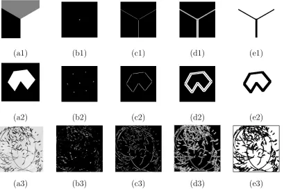
Figure 3.7 (a) Representative points on the test image. (b) Shearlet Trans-form pattern s(ℓ), as a function of ℓ for the points indicated in (a). . . 50 Figure 3.8 (a1-a3) Test images. ((b1-b3) Identification of corners and
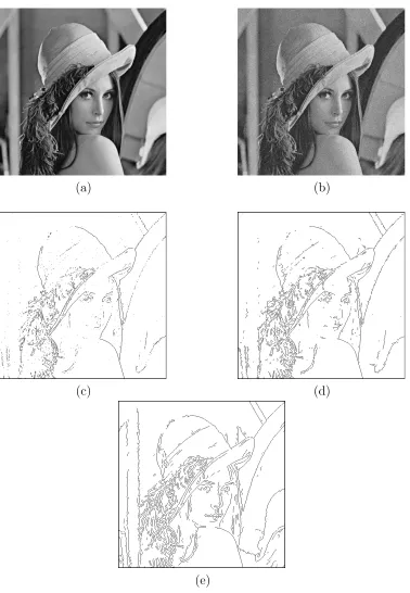
junc-tions. ((c1-c3) Identification of smooth edge points. ((d1-d3) Iden-tification of points near the edges. ((e1-e3)Identification of regular points (smooth regions). . . 54 Figure 3.9 Results of edge detection methods. From (a) to (e): (a)
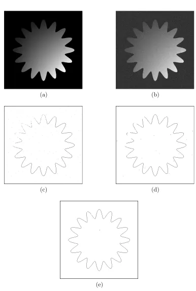
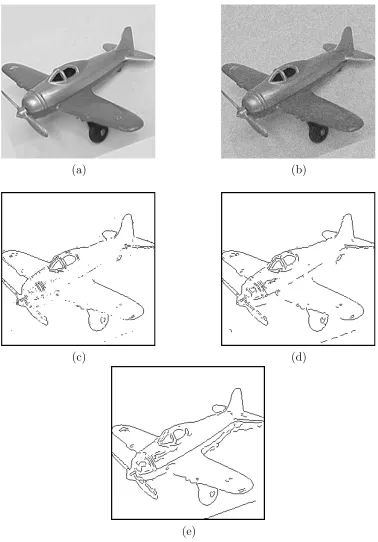
Orig-inal image, (b) noisy image (PSNR=24.61 dB), (c) Sobel result (FOM=0.79), (d) wavelet result (FOM=0.88), (e) shearlet result (FOM=0.92). . . 58 Figure 3.10 Results of edge detection methods. From (a) to (e): (a)
Orig-inal image, (b) noisy image (PSNR=24.58 dB), (c) Sobel result (FOM=0.54), (d) wavelet result (FOM=0.84), and (e) shearlet re-sult (FOM=0.94) . . . 59 Figure 3.11 Edge detection based on a linear fit to the decay of{log|Mw
n[n1, n2]|}Jn=1 and{log|Mn[n1, n2]|}Jn=1. From left to right: Noisy image (PSNR=22.08 dB), edges found analyzing the wavelet transform, and edges found analyzing the shearlet transform. . . 60 Figure 3.12 Results of edge detection methods. From (a) to (e): (a)
Orig-inal image, (b) noisy image (PSNR=24.61 dB), (c) Sobel result (FOM=0.32), (d) wavelet result (FOM=0.60), and (e) shearlet re-sult (FOM=0.89) . . . 61 Figure 4.1 The original shape sequence for activity: Running. . . 75 Figure 4.2 The embedding of a shape sequence in Figure 4.1 into R3. . . . . 76 Figure 4.3 (a) The original shape sequence; (b) The embedding into R3; (c)
The reconstruction of the shape sequence from the embedding curve inR3. . . . 77 Figure 4.4 (a) A original shape sequence; (b) The embedding into R3; (c)
the reconstruction of the shape sequence from its corresponding embedding curve in R3. . . . 78 Figure 4.5 (a) A original shape sequence; (b) The embedding into R3; (c)
The reconstruction of the shape sequence from its corresponding embedding curve in R3. . . . 79 Figure 4.6 (a) A original shape sequence; (b) The embedding into R3; (c)
The reconstruction of the shape sequence from its corresponding embedding curve in R3. . . . 80 Figure 4.7 The reconstruction result for original sequence in Figure 4.1 with
Figure 4.8 Generated sequence start from a circle with walking dynamic. . . 82
Figure 4.9 Generated sequence start from a square with walking dynamic. . 82
Figure 4.10 Generated sequence start from a triangle with walking dynamic. . 83
Figure 4.11 Generated sequence start from a triangle with walking dynamic. . 84
Figure 4.12 Conceptual illustration of the subspace learning from training se-quence. The two red curve denoted as Y1 t , Yt2are the training se-quence while the dark curve denoted as Xt is the testing sequence. The optimal frame, as defined in 4.3 at TY1 0M, TY02M are parallel transported toTX0M along two geodesic curves connectingX0 with each ofY1 0, Y02. . . 86
Figure 4.13 The tracking result for walking. . . 89
Figure 4.14 The tracking result for walking. . . 90
Figure 4.15 The tracking result for walking. . . 91
Figure 5.1 The original shape manifold isM,the ambient space ofM isA(L2). The approximation shape manifold ˆM and its ambient spaceA(S) is a submanifold of M and A(L2). Mˆ is also the intersection of A(s) and M. . . 97
Figure 5.2 implementation of σ : (a) the basis in the ambient space, which yields Bi as the result of Gram Schmidt procedure (b) the fourier approximation of Bi by BSi. . . 104
Figure 5.3 Curve development of Xt ∈ M in RN=30: (a) The original shape sequence represented by angle functionsXt; (b) The horizontal lift U1, U2, U3; and (c) The development (Ut)−1dXt. . . 115
Figure 5.4 The evolutionary spectrum of kWtk: a1, a2, a3 are the EPSD corresponding to the original shape sequence (a), (b), (c) in Figure 5.3. . . 116
Figure 5.5 Distance matrix of data base in [64]. . . 116
Figure 5.6 Distance matrix of CMU Mobo data base. . . 117
Figure 5.7 Nonstationary time series segmentation: (a),(b),(c) is the segmen-tation results of activity bending, running, skipping. . . 117
Figure 5.8 Distance matrix for database in [64]. . . 118
Chapter 1
Introduction
1.1
Motivation
Shape has been well studied and widely utilized as a critical feature for many vision techniques, such as object recognition [1], contour tracking [2] and facial recognition [3]. The previous shape analysis [4, 5, 6] concentrated on how to compare two different shapes, mathematically a metric study of shape. However, the dynamics of shape only received attention recently in the application of human activity modeling [7], [8], [9]. In the current work of shape dynamic analysis there are a few problems, as listed in the following, which still need to be improved.
1. The linear assumption of a nonlinear shape space.
2. The distortion due to the projection from shape manifold to flat space.
3. Computation and invertibility of dimensional reduction of shape dynamics.
In detail, the above problems are explained as follows. In [2] the shape space is globally approximated by a vector space spanned by a modified B-spline basis. Such approximation indeed simplifies the shape dynamics formulation, however, violates the nonlinearity of the underlying shape space as indicated in [4, 5, 6]. In [7] a nonlinear shape space formulation in [5] is adapted however the landmark based shape representation is problematic for general shape dynamics when the landmark is not available or well defined. In addition, in [7], an orthogonal projection is applied to regress the manifold dynamics to flat space, which distorts the original metric and one-one correspondence on other shape manifolds, which is not based on landmarks [4, 6].
Motivated by the current problem of shape dynamic analysis and its urgent need in many vision technologies, in this thesis we concentrate on the problem of how to effectively represent, model and recognize the shape dynamics. Practically in a vision system, the study of shape dynamics is based on segmentation and tracking, for example, how to extract the robust shape features and how to carry out contour tracking. Most of the existing shape analysis techniques assume the perfect segmentation results. In this dissertation, I developed a systematic view of shape dynamic analysis by addressing the problem through different levels: (1) the bottom level segmentation in an image, (2) the middle level shape tracking, dimension reduction, (3) the high level shape dynamic modeling, recognition. The contributions of this dissertation are summarized as follows:
1. An efficient one-one mapping of a manifold valued dynamics to a Euclidean valued dynamics is proposed in Chapter 5.
3. An invertible and computationally efficient dimension reduction for shape dynamics is proposed in Chapter 4.
4. A contour tracking based on the proposed shape dynamic modeling on shape man-ifolds is proposed in Chapter 4.
5. An edge feature extraction with Shearlet transformation is proposed in Chapter 3.
1.2
Organization and Publications
The rest of the dissertation will be organized as follows. In Chapter two, the mathematical backgrounds of this thesis is briefly reviewed. In Chapter three, the feature extraction of edges in an image is discussed. A singularity analysis in shearlet domain is proposed, which better captures the multi-orientation singularities of different types of edge points, for example, edge points on a single edge path and edge points that join different edge paths. This part of the work was also published at,
1. “A Shearlet Approach to Edge Analysis and Detection”, Sheng Yi, Demetrio La-bate, Glenn R. Easley, Hamid Krim,IEEE Transaction on Image Processing, Vol 18, No 5, May, 2009, pp 929-941.
2. “Edge Detection and Processing using Shearlets” Sheng Yi, Demetrio Labate, Glenn R. Easley, Hamid Krim, Proceedings of IEEE International Conference on Image Processing (ICIP), 2008, pp 1148.
in Chapter two. The dimension reduction proposed is invertible and more efficient in computation in comparison to other related works in dimension reduction of curves on manifolds. This part of the work is prepared for publication as follows:
1. “A Invertible Dimension Reduction of Curves on a Manifold”, Sheng Yi, Hamid Krim and Larry K. Norris, Proceedings of IEEE Workshop on Information Theory in Computer Vision and Pattern Recognition, 2011.
2. “A Lower Dimensional Representation of Dynamics on Shape Manifolds”, Sheng Yi, Hamid Krim and Larry K. Norris,IEEE Transaction on Image Processing, 2011
In Chapter five, with the segmentation and tracking results from the techniques in Chapter two and three, the shape dynamics of human activities are studied by regressing a manifold valued random process back to a flat space with a stochastic curve develop-ment. This should be compared with other techniques based on projections to tangent space. Such mapping from a manifold to a Euclidean space generally hold one-one corre-spondence for any differentiable manifold. Based on the proposed mapping to a Euclidean space, we build a Brownian motion model for the resulting random process in a Euclidean space, which well captures the original shape dynamics of human activities. This part of the work is also published as follows:
1. “Human Activity Modeling on Shape Manifold”, Sheng Yi, Hamid Krim, Larry K. Norris, Proceedings of Eurographics Workshop on 3D Object Retrieval, 2011.
And a Journal submission is currently under review,
1. “Human Activity Analysis as Random Process on Shape Manifold”, Sheng Yi, Hamid Krim, Larry K. Norris, IEEE Transaction on Image Processing, 2011 (sub-mitted)
Chapter 2
Background
This thesis utilizes some recent developments in mathematics and statistics, such as, composite wavelet theory, shape analysis, Bayesian filtering and manifold geometry. To make the dissertation self-contained for reading, in this chapter the necessary theoretical foundations are briefly introduced.
2.1
Review of Wavelet Framework for Image
Analy-sis
In the view point of dimensionality, the recent evolution of wavelet theory is essentially the extension from a low dimension to a high dimension, from isotropic to directional. Early on, most 1D wavelet basis is constructed for 1D signal processing. With the tra-ditional 1D wavelet basis application to image processing, a direct extension is made from 1D wavelet to 2D wavelet, as a separable basis. However, facing the lack of char-acterization of orientation selectivity, many oriented wavelet basis are proposed such as Gabor wavelet and Steerable filter [16, 17]. Further more, to better characterize the line-wise singularity [18, 19], Shearlet [20, 21], and Curvelet[22, 23] are constructed to systematically justify the problem of how to better represent edge in image.
In Chapter 3, the proposed image feature extraction is under the Shearlet transforma-tion. To review and compare with other popular wavelet base, we first lay out theoretical formulation of wavelet and frame theory. The definition of wavelet function is as in [24]:
Definition 1 A wavelet is a function ψ ∈L2(R) with zero average:
Z +∞ −∞
ψ(x)dx= 0. (2.1.1)
such that kψk= 1. A family of wavelet basis functions derived fromψ with scalinga and dilation t is:
ψa,t = √1
aψ( x−t
a ). (2.1.2)
The wavelet transformation of f ∈L2(R) at scale a and position t is,
W f(a, t) =
Z +∞ −∞
f(t)√1
aψ
∗(t−x
a )dx. (2.1.3)
representation of a function f in terms of the dual wavelet basis:
f =X
n
< f, ψn >ψ˜n. (2.1.4)
In most image representation problems, for example image compression, the complete-ness of representation is very important. In frame theory [24] the following admissible condition is derived to test if a wavelet functions ψnn∈Γ is a complete basis of a signal space.
Definition 2 (Admissible Frame) The sequence ψnn∈Γ is a frame of H if there exist two constants A >0 and B >0 such that for any f > H
Akfk2 ≤X n∈Γ
|< f, ψn >|2 ≤Bkfk2. (2.1.5)
Given the above frame condition satisfied, there exists a dual frame ˜ψ such that the complete reconstruction from the wavelet coefficients of the original signal is possible. The following theorem describes in detail how to carry out the reconstruction.
Theorem 2.1.1 (Reconstruction with Dual Basis) suppose that ψnn∈Γ is a frame with frame bounds A and B. Let ψ˜be the dual basis of ψ. For any f ∈H,
1
Bkfk
2
≤X
n∈Γ
|< f,ψn˜ >|2 ≤ 1 Akfk
2, (2.1.6)
and
f =X
n∈Γ
2.1.1
Separable Wavelet: A Direct Extension from 1D to 2D
A direct product of two one dimensional wavelets bases leads to a simple extension to a two dimensional wavelet basis. Given any two one dimensional wavelet basis ψxj,n(j,n)∈Z2
and ψyl,m
(j,n)∈Z2 of L
2(R), one can create 2D wavelet basis as follows:
ψxyj,n,l,m=ψj,nx ψl,my . (2.1.8)
2.1.2
Shearlet: A special case of Composite Wavelet
The definition of a composite wavelet is as followsψp,k =ψ(Gp(x−Cpk)), (2.1.9)
where p∈ P,Gp and Cp are invertible matrixes.
Shearlet is a special case of composite wavelet framework. Let G be a subgroup of the group of 2×2 invertible matrices. The affine systems generated by ψ ∈ L2(R2) are the collections of functions
ψM,t(x) =|detM|−
1
2ψ(M−1(x−t)), t∈R2,M∈G. (2.1.10)
If any u∈L2(R2) can be recovered via the reproducing formula
u=
Z
Rn
Z
Gh
u, ψM,tiψM,tdλ(M)dt,
wavelet transform is the mapping
u→Wψu(M, t) =hu, ψM,ti, (2.1.11)
for (M, t)∈G×R2.
The separable wavelet is also a special case of the composite wavelet with the matrix
M as aI, where a > 0 and I is the identity matrix. In this situation, one obtains the isotropic continuous wavelet transform:
Wψu(a, t) =a−1
Z
R
u(x)ψ(a−1(x−t))dx,
where the dilation factor is the same for all coordinate directions. This is the “standard” wavelet transform used in most wavelet applications (including the wavelet-based edge detection by Mallat et al. [24] described in Chpater 3).
It is well known that the continuous wavelet transform has the ability to identify the singularities of a signal. In fact, if a function uis smooth apart from a discontinuity at a pointx0, then the continuous wavelet transformWψu(a, t) decays rapidly asa→0, unless
(2.1.11) called thecontinuous shearlet transform. This is defined as the mapping
SHψu(a, s, t) = hu, ψasti, (2.1.12)
whereψast(x) =|detMas|−12ψ(M−1
as (x−t)), andMas =
a−√as
0 √a
fora >0, s∈R, t∈R2. Observe thatMas =BsAa, whereAa=a 0
0√a
and Bs =1−s 0 1
. Hence to each matrix
Mas are associated two distinct actions: an anisotropic dilation produced by the matrix
Aa and a shearing produced by the non-expansive matrix Bs.
H H Y
(a, s) = (1 32,1)
@ @ R
(a, s) = (14,0)
6
(a, s) = ( 1 32,0)
ξ1 ξ1
ξ2 ξ2
@ @@R
@ @ R
(a, s) = (14,0)
@ @ I
(a, s) = (1 32,0)
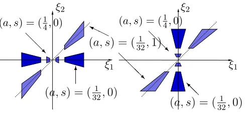
Figure 2.1: Frequency support of the horizontal shearlets (left) and vertical shearlets (right) for different values ofa and s.
The generating function ψ is a well localized function satisfying appropriate admissi-bility conditions [18, 19], so that each u∈L2(R2) has the representation
u= Z R2 Z ∞ −∞ Z ∞ 0 h
u, ψastiψast da a3 ds dt.
smooth functions with supp ˆψ1 ⊂[−2,−12]∪[12,2] and supp ˆψ2 ⊂[−1,1]. In addition, to obtain the edge detection results presented in the next section, ˆψ1 (respectively, ˆψ2) is assumed to be odd (respectively, even). In the frequency domain:
ˆ
ψast(ξ1, ξ2) =a
3
4 e−2πiξtψˆ1(a ξ1) ˆψ2(a−12(ξ2
ξ1 −s)),
and, thus, each function ˆψast is supported on the set
{(ξ1, ξ2) :ξ1 ∈[−2a,−21a]∪[21a,2a], |ξξ21 −s| ≤√a}.
Thus each shearlet ψast has frequency support on a pair of trapezoids, at various scales, symmetric with respect to the origin and oriented along a line of slopes. As a result, the shearlets form a collection of well-localized waveforms at various scales a, orientations s
and locations t.
Notice that the shearing variable s corresponds to the slope of the line of orientation of the shearlet ˆψast, rather than its angle with respect to the ξ1 axis1. It follows that the shearlets provide a nonuniform angular covering of the frequency plane when the variablesis discretized, and this can be a disadvantage for the numerical implementation of the shearlet transform. To avoid this problem, the continuous shearlet transform is modified in [18, 19] as follows. In the definition of SHψ, given by (2.1.12), the values
of s will be restricted to the interval [−1,1]. Under this restriction, in the frequency plane, the collection of shearlets ψast will only cover the horizontal cone {(ξ1, ξ2) : |ξξ21| ≤ 1}. To compensate for this, a similarly defined second shearlet transform is added,
1The curvelets are indexed by scale, angle and location, where the angle is the angle of orientation in
whose analyzing elements are the “vertical” shearlets ψ(1)ast. In the frequency plane they are obtained from the corresponding “horizontal” shearlets ψast through a rotation by
π/2. The frequency supports of some representative horizontal and vertical shearlets are illustrated in Figure 1. By combining the two shearlet transforms, any u ∈ L2(R2) can be reproduced with respect to the combination of vertical and horizontal shearlets. In the rest of the dissertation, when it will be needed to distinguish the two transforms the notation SH(0)ψ is used(respectively, SHψ(1)) for the continuous shearlet transform associated to the horizontal cone (respectively, the vertical cone).
2.2
Review of Shape Space
The shape space has been of great interest to both mathematics and engineering com-munities. The first formulation of shape space can be traced back to Kendal’s work [5] in 1984. After Kendal’s landmark based shape representation, different shape spaces are developed by adapting to different shape representations. For example, in [4] the shape is represented by the angle function of the arclength parameterized curve and in [6] the shape is considered to be a smooth embedding fromS1 toR2. In this section, in addition to the Kendal’s shape space, two recent developments of shape space in [6] [4] is also reviewed.
2.2.1
Kendal’s Shape Manifold
The shape manifold is defined in [5] as a quotient space
where (Rm)k−1 is the space of the k landmark in Rm, and Sim represent the similarity
transformation including, translation, rotation and scaling in Rm. The zero shape is
excluded from (Rm)k−1 to avoid degeneration of all the landmarks to a single point. In terms of the coordinates of landmarks in R2, the shape manifold can be described as invariants to similarity transformations. Let the k landmark be represented by the vector X
X= (x1, x2,· · · , xk), (2.2.14)
where, ∀i, xi ∈R2.
By normalizing the size of X, and translating the mean of X to zero, the preshape
Z ∈Sk
m is invariant to scaling and translation.
Z = X−X¯
||X−X¯||. (2.2.15)
Given the fact that kZk= 1, the preshape space Sk
m is a sphere of dimension m(k−1)
The left invariancy to rotation could be formulated as quotient preshape space on the rotation group SO(m)
Σkm =Smk/SO(m). (2.2.16)
Kendal in [5] showed that the quotient metric of Σk
m is explicitly related to the metric
on the preshape space. LetpW1, pW2 be two points on Σkm, as the projection of two point W1, W2 on preshape space Smk. The distance between two points pW1, pW2 on Σkm can be
written as the following.
ρ(pW1, pW2) = inf
Thus instead of working directly on the quotient space Σk
mmost of the existing techniques
take advantage of the simple geometry of Sk m.
2.2.2
Klassen’s Shape Manifold
According to [4], a planar shape is a simple and closed curve in R2,
α(s) :I →R2, (2.2.18)
where an arc-length parameterization is adopted. A shape is represented by a direction index function θ(t). With such a parameterization, θ(s) may be associated to the shape by
∂α ∂s =e
jθ(s). (2.2.19)
The ambient space of the manifold of θ is an affine space based on L2. Thus
θ∈A(L2). (2.2.20)
The restriction of a shape is that it must be a closed and simple curve, and invariant over rigid Euclidean transformations. The shape manifoldM is defined by a level function
φ as
φ(θ) =
Z 2π
0
θds,
Z 2π
0
cos(θ)ds,
Z 2π
0
sin(θ)ds
. (2.2.21)
M =φ−1(π,0,0). (2.2.22)
computation possible,
TθM ={f ∈L2|f ⊥ span{1,cos(θ),sin(θ)}}. (2.2.23)
In addition, an iterative projection is proposed in [4] to project the point in ambient space back to the shape manifold M. The idea is that each timeθ is updated asθ+dθ, wheredθ is orthogonal to the level setφ−1(φ(θ)). The dθ is calculated asdφ−1((π,0,0)−
φ(θ)). For the detailed form of the Jacobian ofdφ, one could refer to [4].
The problem of this manifold for our stochastic modeling is the infinite dimension. The mapping of random process in [26] from a manifold to a flat space is only defined on a finite dimensional manifold. Therefore, in Chapter 4, a Fourier approximation of the shape manifold we discussed above is developed, such that the dimension is reduced to a finite number.
2.2.3
Michor’s Shape Manifold
In [27, 6], the shape manifold is considered to be the quotient of the space of planar curve by similarity transformations and parameterizations. The curve space construction in [27] is base on the work in [6], in which the simple and closed curve is represented by a embedding from S1 to R2. Accordingly the curve space is defined as the base manifold
Be(S1, R2) of the principle bundle (Emb(S1, R2),Diff(S1))
where Emb(S1, R2) are embeddings from a circle S1 to R2, which implyies that the embedding result in R2 is simple and closed. The quotient factor Dif f(S1) are dif-feomorphisms from circle to circle, which represent the reparameterization effect. Thus
Be(S1, R2) represents a simple and closed planar curve which is invariant to reparame-terization.
The geodesic in the quotient space Be(S1, R2) is derived out of the horizontal field. The horizontal field at c ∈ Emb(S1, R2) is defined as a vector field h along c(θ) such that,
h,∂c ∂θ
= 0. (2.2.25)
Letc(t, θ) be a path in Be(S1, R2). Then the geodesic equation for c(t, θ) is a immediate result from horizontal field as the following,
∂c ∂t,
∂c ∂θ
= 0. (2.2.26)
In this work the metric on the quotient space Be(S1, R2) is projected fromH0 metric [6] in Emb(S1, R2) by horizontal lifting.
2.2.4
Comparison of Different Shape Spaces
However in [6], the principle bundle structure is not a frame bundle and it is hard to effectively formulate the frame bundle on this particular manifold. Thus in this thesis, we follow the shape space setting in [4] in the rest of the thesis.
2.3
Bayesian Filtering Framework
Bayesian Filtering solves the ill-posed inverse problem for dynamical system such as prediction and smoothing. The development of filtering method for a dynamic system has a long history as documented in [28]. This section focus on the Kalman Filter, and its extension to nonlinear condition. The Particle Filter is not considered in this work because of the high dimensionality of the shape space.
2.3.1
Kalman Filter
The discrete Kalman filter [28] is a estimation of a random processxkwhich is the solution of the following linear differential equations.
State Equation:
xk =Axk−1+Buk−1+wk. (2.3.27)
Observation Equation:
zk=Hxk+vk. (2.3.28)
wherewk∼N(0, Q) andvk∼N(0, R) are white noises. ukis the optional input process,
and zk is the observation.
Ac-cording to [29],
P(xk|zk) =N(ˆxk, Pk). (2.3.29)
Obviously the mean ˆxkis the Beyesian estimation for xk. Through linear calculation, the closed form of ˆxk is
ˆ
xk = ˆx−k +Kk(zk−Hxˆ−k), (2.3.30)
where ˆx−k is the initial estimation given xk−1:
ˆ
x−k =Axk−1+Buk. (2.3.31)
In addition the coefficient Kk provides a proper correction from observation error (zk− Hxˆ−k) to the initial estimation.
Kk=Pk−HT(HPk−HT +R)−1, (2.3.32)
where
Pk− =APk−1AT +Q, (2.3.33)
and
Pk = (1−KkH)Pk−. (2.3.34)
Recall the posterior probability P(xk|zk) in Equation (2.3.29), the covariance matrixPk
2.3.2
Extended Kalman Filter
One of the limitations of the discrete Kalman filter discussed in the previous subsection is that the linear assumption of the state and observation function as shown in Equations (2.3.28) and (2.3.27). The goal of Extended Kalman filter is to generalize the Kalman filtering to the nonlinear processes. The core idea is to use the first order derivative to linearly approximate the increments of the state and observation functions.
In contrast to the state and observation function in Equation 2.3.28 and 2.3.27, the nonlinearity is considered here, by introducing a non-linear stochastic difference equation.
xk =f(xk−1, uk−1, wk), (2.3.35)
zk=h(xk, vk). (2.3.36)
The linearization of the above two equations at time k is as follows: let ˆxk =f(xk−1,0) and ˆzk =h(xk,0). Then the state Equation (2.3.35) can be written as
xk≈xkˆ +A(xk−1−xkˆ −1) +W(wk−1−0), (2.3.37)
where
Aij = ∂fi
∂xj(ˆxk−1, uk−1,0), (2.3.38)
and
Wij = ∂fi
∂wj
Similarly for the observation function,
zk≈zˆk+H(xk−1−xˆk−1) +V(vk−1−0), (2.3.40)
where
Hij = ∂hi
∂xj(ˆxk−1, uk−1,0), (2.3.41)
vij = ∂hi
∂vj(ˆxk−1, uk−1,0). (2.3.42)
With the linear approximation in Equation (2.3.40), the estimation of xk is regressed to
the linear problem as in previous subsection.
2.4
Geometry and Stochastic Analysis on Manifolds
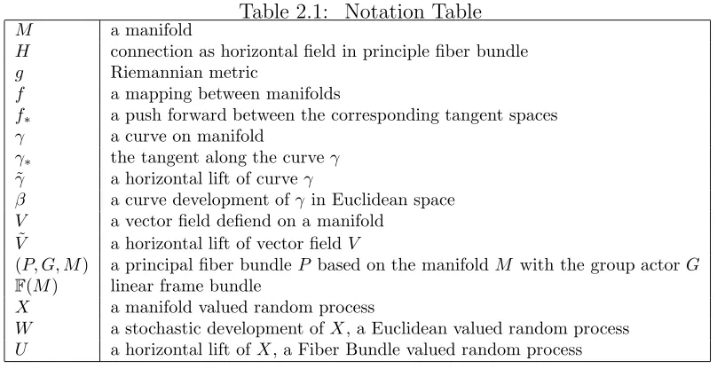
Table 2.1: Notation Table
M a manifold
H connection as horizontal field in principle fiber bundle
g Riemannian metric
f a mapping between manifolds
f∗ a push forward between the corresponding tangent spaces
γ a curve on manifold
γ∗ the tangent along the curveγ
˜
γ a horizontal lift of curve γ
β a curve development ofγ in Euclidean space
V a vector field defiend on a manifold
˜
V a horizontal lift of vector fieldV
(P, G, M) a principal fiber bundle P based on the manifoldM with the group actor G
F(M) linear frame bundle
X a manifold valued random process
W a stochastic development of X, a Euclidean valued random process
U a horizontal lift of X, a Fiber Bundle valued random process
2.4.1
Connection on Manifolds
To study a random process on a manifold, the difficulty resulting from the curvature of the manifold needs to be overcomed. For example, to define a Brownian motion process
Xt on a manifold M, one may define a vector field V ∈ T M and Euclidean Brownian motion Z as the driving process as
Xt =X0+
Z t
0
X
i
Vi(Xs)Zids. (2.4.43)
Such modeling considers Xt as a solution of SDE(X0, V, Z). The incremental of Xt is unique in terms of the distribution estimation from data. However the selection of V
and Z is not unique. From a geometric view in [26], one can select the vector field V
by the concept of connection. A connection defines the relations among tangents along a curve on a manifold. Such a relation may be used to determine the parallelism of two tangent vectors in two different tangent spaces. Mathematically there exist many valid connections for a particular manifold. In Chapter 4 and 5, two particular connections are developed on a shape manifold: one is a flat connection defined as a cross section in a frame bundle and the other one is a nonflat connection as a Levi-Civita connection with the metric induced from the ambient space of the shape manifold. Specifically, we can set up a parallelism between different tangent spaces by defining a ”standard basis” in each tangent space, and by then declaring these standard bases to be parallel. Such a form of connection is much simpler to calculate and takes place in a so-called principal fiber bundle as a horizontal distribution.
The frame bundle F(M) [26] will be encountered in the following sections is a special
case of a principal bundle.
Definition 3 (Principal Fiber Bundle) As in [30] a principal fiber bundle is a set
(P, G, M), where P, M are C∞ manifolds, and G is a Lie group such that
(1) G acts freely on the right of P, P ×G →P. For g ∈ G, we shall also write Rg for
the map defined by g
(2) M is the quotient space of P by an equivalence relation under G (any shape subjected
to a g ∈G is equivalent to itself ), and the projection π:P →M isC∞, so for m ∈M,
G is simply transitive on π−1(m)
(3) P is locally trivial. Thus for any open set U ⊂M, π−1(U)∼U×G.
structure in P. For any point m ∈ M, we have a equivalent class of π−1(m), in which one can ”move up and down” by applying group element g ∈G. In Figure 2.2 the fiber structure is illustrated as a line in the cube corresponding to a point in a manifold. One example of a principal bundle is the orthogonal frame bundle F(M) of a n-dimensional manifold. F(M) will be extensively used in this dissertation. A point u inF(M) can be
written as
u= (x, b) (2.4.44)
wherem ∈M andb =e1, e2, ..., en is an orthogonal basis of the associated tangent space
TmM. The group Gacting on a fibre is SO(n))
Referring to the definition of a principal bundle, the equivalent class for each point
m ∈M is all the orthogonal basis for the tangent space TmM. The rotation matrix can
be utilized to transform one basis to another.
Definition 4 (Connection) A connection [30] on the principal bundle (P, G, M) is a
n-dimensional distribution H on P, where n=dim(M), such that (1) H ∈C∞
(2) for every p∈P,Hp+Vp =TpP, where Vp is the vertical space andHp is a horizontal
space of TpP. A vector Y ∈TpP is vertical if π∗(Y) = 0 (3) for every p∈P, g ∈G, (Rg)∗(Hp) =Hpg.
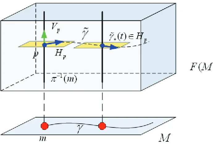
a result, we discover the appropriate distribution2 of bases along the curve accomplishing the parallel transport of a shape to its next evolution in the sequence. With the parallel bases along a curve, the tangent of a curve can be represented by its corresponding coefficients. By preserving the coefficients, we can move all the tangents to a single tangent plane. Such an operation is called a parallel transport along a curve. If we reintegrate all the parallelly transported tangents in that single tangent plane, we have a curve in the flat space. This is referred to as a curve development in the tangent plane. Figure 2.2 illustrates the definition of H in one particular principal fiber bundle, the frame bundleF(M). Hp could be understood as a subspace ofTpF(M) which is smoothly defined for all p∈F(M).
Definition 5 (Horizontal Lift) Let γ be a piecewise C∞ curve in M, γ : [0,1]→ M.
Let p ∈ π−1(γ(0)). According to [30], then there exists a unique lift γ˜ of γ such that ˜
γ∗(t)∈H˜γ(t) and γ˜(0) =p. We say that γ˜ is the horizontal lift of γ that starts at p∈P.
Definition 6 (Curve Development with orthogonal frames) Let γ be a piecewise
C∞ curve in M starting at m, Ei
j(m) an orthogonal basis at m, where i is the index for
different basis vectors and j is the index for elements of each basis vector. Let γ˜ be the horizontal lift of γ in F(M) with ˜γ = (γ(s), Ei(γ(s))). According to [30], then by writing
β =
Z t
0 ˜
γ−1γ∗ds, (2.4.45)
Figure 2.2: A connectionH as a distribution inF(M),where the yellow plane represents the Hp as the subspace of TpF(M). ˜γ is the horizontal lift of curve γ on manifoldM. ˜γ∗
is the tangent along ˜γ, such that∀t,γ˜∗ ∈Hγ(˜t).
where (˜γ−1γ
∗)i(s) is defined as the following inner product
(˜γ−1γ∗)i(s) = X
j
Eji(γ(s))(γ∗)j(s). (2.4.46)
we define a curve in RN which is called a development of γ into RN with respect to
b. And PiEi
j(γ(s))βi(s) is a curve in TmM called the development of γ in TmM. A
conceptual distribution is illustrated in Figure (2.3)
Definition 7 (Parallel Transport) Let γ be a piecewise C∞ curve in M and let F M
parallel transport of V(γ(t)) from γ(t) to γ(t+h) can be defined as the mapping between tangent planes τ :Tt1M →Tt2M,
τh(V(γ(t))) =γ(^t+h)◦γg(t)
−1
◦V(γ(t)). (2.4.47)
One may parallel transport the vector V(γ(t)) fromγ(t) toγ(t+h) as follows. First find the components of V(γ(t)) with respect to the frame γg(t), namely eγ−1(V(γ(t))). Then use these coefficients to construct the parallel transported vector atγ(t+h) using the parallel transported framee(γ(t+h)), namely γ^(t+h)◦(γg(t)−1◦V(γ(t)))
Figure 2.3: The curve development of γ is R0t < ˜γ(s)−1, γ
∗(s) > ds, where ˜γ(s)−1,˜γ(s)
are the dual basis and basis of TγsM. γ∗ is the tangent along γ ∈M.
A more expanded and detailed discussion of connections may be found in [31] [30].
2.4.2
Stochastic Horizontal Lift and Development
technique is extended to map a manifold valued random process to a Euclidean process. According to [26], a stochastic horizontal lift and its development are defined as follows,
Definition 8 (Stochastic Horizontal Lift and Development) (1)AnF(M)-valued
random process U is said to be horizontal if there exists an Rd-valued semi-functional W
such that,
dUt=
d
X
i=1
Hi(Ut)◦dWti (2.4.48)
where Hi are the fundamental horizontal vector fields that span H.
(2) Let W be an Rd-value random process and U
0 an F(M)-valued, F0-measurement random variable. The solution U of SDE (2.5.49) is called the stochastic development of
W in F(M). Its projection X =πU is called a stochastic development of W in M.
(3)Let X be an M-valued random process. AnF(M)-value horizontal random processU
such that its projection πU =X is called a stochastic horizontal lift of X.
2.5
Stochastic Analysis on Manifolds
The horizontal lift and curve development mentioned in the last section may also be extended to a stochastic setting. According to [26], a stochastic horizontal lift and its development may be defined as follows,
Definition 9 (Stochastic Horizontal Lift and Development) (1)AnF(M)-valued semimartingaleU is said to be horizontal if there exists an Rd-valued semi-functional W
such that,
dUt= d
X
i=1
Hi(Ut)◦dWti (2.5.49)
where Hi are the fundamental horizontal vector fields that span H.
(2)Let W be anRd-value semimartingale and U
0 anF(M)-valued, F0-measurement ran-dom variable. The solution U of SDE (2.5.49) is called the stochastic development of W
in F(M). Its projection X =πU is called a stochastic development of W in M.
(3)Let X be an M-valued semimartingale. An F(M)-value horizontal semimartingaleU
such that its projection πU =X is called a stochastic horizontal lift of X.
2.6
Summary
Chapter 3
Image Feature Extraction with
Shearlet
3.1
Introduction
Edges are prominent features in images and their analysis and detection are an essential goal in computer vision and image processing. Indeed, identifying and localizing edges are a low level task in a variety of applications such as 3D reconstruction, shape recognition, image compression, enhancement and restoration.
is particularly designed to deal with directional and anisotropic features typically present in natural images, and has the ability to accurately and efficiently capture the geometric information of edges. As a result, the shearlet framework provides highly competitive algorithms, for detecting both the location and orientation of edges, and for extracting and classifying basic edge features such as corners and junctions.
Our shearlet approach has similarities with a number of other methods in applied mathematics and engineering to overcome the limitations of traditional wavelets. These methods includecontourlets[34, 35]complex wavelets[36],ridgelets[37] andcurvelets[22]. In contrast to all these methods, the shearlet framework provides a unique combination of mathematical rigidness and computational efficiency when addressing edges, optimal efficiency in dealing with edges, and computational efficiency. In addition, its continuous formulation is particularly well-suited for designing an implementation, presented in this work, for the purpose of edge analysis and detection.
3.1.1
Edge detection using wavelets.
In the classic Canny edge detection algorithm [38], an image u is smoothed by a convo-lution with a Gaussian filter:
ua =u∗Ga, (3.1.1)
heavily depends on the scaling factora [39, 40].
It was observed by Mallat et al. [10, 11] that, at a single scale, the Canny edge detector is equivalent to the detection of the local maxima of the wavelet transform of
u, for some particular choices of the analyzing wavelet. In fact, the function ψ =∇G is a wavelet known as the first derivative Gaussian wavelet. Thus, each imageu ∈L2(R2) satisfies:
u(x) =
Z
Wψu(a, y)ψa(x−y)dy,
where ψa(x) =a−1ψ(a−1x), and Wψu(a, x) is thewavelet transform of u, defined by
Wψu(a, x) =
Z
u(y)ψa(x−y)dy=u∗ψa(x).
The significance of this representation is that the wavelet transform provides a space-scale decomposition of the image u, where u ∈ L2(R2) is mapped into the coefficients
Wψu(a, y) which depend on the location y∈R2 and the scaling variable a >0. Another useful observation is that the wavelet transform of u is proportional to the gradient of the smoothed image ua:
∇ua(x) =u∗ ∇Ga(x) =u∗ψa(x) =Wψu(a, x). (3.1.2)
This shows that the maxima of the magnitude of the gradient of the smoothed image ua
wavelet transform [24].
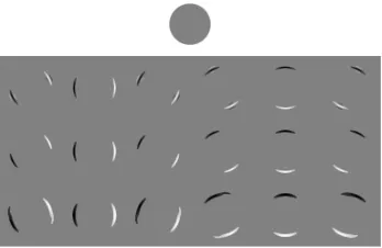
Figure 3.1: Analysis of the edge response. The magnitudes of the shearlet (respectively, wavelet) transform of an edge point on the star-shaped figure (a) are plotted on a log-arithmic scale as a black (respectively, gray) line. Figure (b) shows the response of the shearlet transform when its orientation variable is tangent to the edge. Figure (c) shows the response when the orientation variable is normal to the edge.
The difficulty of edge detection is particularly prominent in the presence of noise, and when several edges are close together or cross each other, e.g., 2–dimensional projections of 3–dimensional objects [41]. In such cases, the following limitations of the wavelet approach (and other traditional edge detectors) become evident:
• Difficulty in distinguishing close edges. The isotropic Gaussian filtering causes edges running close together to be blurred into a single curve.
• Poor angular accuracy. In the presence of sharp changes in curvature or crossing curves, the isotropic Gaussian filtering leads to an inaccurate detection of edge orientation. This affects the detection of corners and junctions.
and curves. For example, in [42, 43, 44] it is proposed to replace the scalable collection of isotropic Gaussian filters Ga(x1, x2), a > 0 in (3.1.1) with a family of steerable and scalable anisotropic Gaussian filters
Ga1,a2,θ(x1, x2) =a
−1/2 1 a−
1/2
2 RθG(a−11x1, a−21x2),
wherea1, a2 >0 andRθ is the rotation matrix byθ. Unfortunately, the design and imple-mentation of such filters is computationally demanding. In addition, the justification for this approach is essentially intuitive, and there is no proper theoretical model to indicate how to “optimize” such family of filters to best capture edges.
3.2
Singularity analysis using the shearlet transform
The continuous shearlet transform is able to precisely capture the geometry of edges. Indeed, the asymptotic decay rate of the continuous shearlet transform SHψu(a, s, t), for
a → 0 (fine scales), can be used to obtain both location and orientation of edges in an imageu. This is a significant refinement with respect to traditional wavelets, which only detect the location. We now present a brief summary of the most relevant results which are useful for our analysis. We refer to [18, 19] for more details.
To model an image, let Ω = [0,1]2 and consider the partition Ω =SL
n=1Ωn∪Γ, where: 1. each “object” Ωn, for n= 1, . . . , L, is a connected open set (domain);
2. the set of edges of Ω be given by Γ =SLn=1∂ΩΩn, where each boundary ∂ΩΩn is a
smooth curve of finite length.
form
u(x) =
L
X
n=1
un(x)χΩn(x) for x∈Ω\Γ
where, for each n = 1, . . . , L, un ∈ C1
0(Ω) has bounded partial derivatives, and the sets Ωn are pairwise disjoint in measure. Foru∈I(Ω), it yields the following results.
Theorem 3.2.1 If t /∈ Γ, then
lim
a→0a
−34 SH
ψu(a, s, t) = 0. (3.2.3)
If t ∈ Γ and, in a neighborhood of t = (t1, t2), the boundary curve is parametrized as (E(t2), t2), and s6=−E′(t
2), then also (3.2.3) holds. Otherwise, if s=−E′(t2), there is a constant C >0 such that
lim
a→0a
−34 SHψu(a, s, t) =C|[u]
t|,
where [u]t is the jump of u at t, occurring in the normal direction to the edge.
This shows that asymptotic decay of the continuous shearlet transform of u is the slowest for t on the boundary of Ω, and s corresponding to the normal orientation to Ω att (see Figure 3.1). Other useful results from [18, 19] are the following:
• If u ∈ I(Ω) and t is away from the edges, then SHψu(a, s, t) decays rapidly as
a→ 0, and the decay rate depends on the local regularity of u. In particular, if u
is Lipschitz–α near t0 ∈R2, then the following estimates hold: for α≥0,
|SHψu(a, s, t0)| ≤C a
1
while for α <0,
|SHψu(a, s, t0)| ≤C a(α+34), as a→0.
We refer to [24] for the definition of Lipschitz regularity. Classification of points by their Lipschitz regularity is important as it can be used to distinguish true edge points from points corresponding to noise [10, 11].
• If u contains a corner point, then locally, as a → 0, SHψu(a, s, t) decays as a3/4
when s is the direction normal to the edges. It decays asa5/4 otherwise.
• Spike-type singularities produce a different behavior for the decay of the shearlet transform. Consider, for example, the Dirac delta centered at t0. Then
|SHψδt0(a, s, t0)| ≍a−
3/4, as a →0,
so that the transform actually grows at fine scales. The decay is rapid for t6=t0.
These observations show that the geometric information about the edges of u can be completely resolved by looking at the values of its continuous shearlet transform SHψu(a, s, t) at fine scales. Additionally, similar to the wavelet case, the behavior of
3.3
Computational nature of shearlet transformation
A numerically efficient implementation of the shearlet transform was previously intro-duced in [45]. It was based on the use of a Laplacian pyramid combined with appropriate shearing filters. That particular implementation, however, was specially designed for im-age denoising. Since its direct application to edge detection suffers from large sidelobes around prominent edges (which is the same problem with the curvelet implementations), a different implementation will be presented here. This new implementation is based on separately calculating the vertical and horizontal shearlets and is amenable to a continu-ous (non-dyadic) scaling. For its development, consistent with the theoretical analysis in [19], special properties on the shearlet generating functionψ (see Chapter 2) are utilized. We start by reformulating the operations associated with the shearlet transform in a way which is suitable to its numerical implementation. Forξ = (ξ1, ξ2)∈Rb2,a <1, and |s| ≤1, let
b
w(0)a,s(ξ) = a−
1
4 ψˆ2(a−12 (ξ2
ξ1 −s))χD0(ξ)
b
wa,s(1)(ξ) = a−14 ψˆ2(a−12 (ξ1
ξ2 −s))χD1(ξ),
where D0 = {(ξ1, ξ2) ∈ Rb2 : |ξξ21| ≤ 1}, D1 = {(ξ1, ξ2) ∈ Rb2 : |ξξ12| ≤ 1}. For a < 1, |s| ≤1, t∈R2, d= 0,1, the Fourier transform of the shearlets can be expressed as
ˆ
ψ(a,s,td) (ξ) = a V(d)(a ξ)wb
(d)
a,s(ξ) e−2πiξt,
where V(0)(ξ
u∈L2(R2) is:
SH(ψd)u(a, s, t) =a
Z
ˆ
u(ξ)V(d)(a ξ)wba,s(d)(ξ)e2πiξtdξ, (3.3.4)
whered= 0,1 correspond to the horizontal and vertical transforms, respectively. Hence, from (3.3.4) it yields that
SHψ(d)u(a, s, t) =va(d)u∗w(a,sd)(t) (3.3.5)
where
va(d)u(t) =
Z
R2
auˆ(ξ)V(d)(aξ)e2πiξtdξ.
To obtain a transform with the ability to detect edges effectively, the functions ˆψ1 is chosen to be odd and ˆψ2 to be even.
We are now ready to derive an algorithmic procedure to compute a discrete version of (3.3.5). ForN ∈N, anN×N image can be considered as a finite sequence{u[n1, n2] :
n1, n2 = 0, . . . , N −1}. Thus, identifying the domain with Z2N, ℓ2(Z2N) is viewed as
the discrete analog of L2(R2). Consistently with this notation, the inner product of the images u1 and u2 is defined as
hu1, u2i=
NX−1
n1=0
NX−1
n2=0
u1[n1, n2]u2[n1, n2],
and, for −N/2 ≤ k1, k2 < N/2, its 2D Discrete Fourier Transform (DFT) ˆu[k1, k2] is given by:
ˆ
u[k1, k2] = 1
N N−1
X
n1,n2=0
u[n1, n2]e−2πi(
n1
Nk1+nN1k2).
(·,·) denote function evaluations. We shall interpret the numbers ˆu[k1, k2] as samples ˆ
u[k1, k2] = ˆu(k1, k2) from the trigonometric polynomial ˆu(ξ1, ξ2) =PNn1−,n12=0u[n1, n2]e
−2πi(nN1ξ1+nN1ξ2).
To implement the directional localization associated with the shearlet decomposition described by the window functions w(a,sd), the DFT will be computed on a grid consisting
of lines across the origin at various slopes called the pseudo-polar grid, and then apply a one-dimensional band-pass filter to the components of the signal with respect to this grid. To do this, let us define the pseudo-polar coordinates (ζ1, ζ2)∈R2 by:
(ζ1, ζ2) = (ξ1,ξξ21) if (ξ1, ξ2)∈ D0; (ζ1, ζ2) = (ξ2,ξξ12) if (ξ1, ξ2)∈ D1.
Using this change of coordinates, the following result is obtained.
g
ˆ
va(d)f(ζ1, ζ2) = ˆv(ad)f(ξ1, ξ2),
gˆ
w(d)(a−1/2(ζ
2−s)) = wˆa,s(d)(ξ1, ξ2).
This expression shows that the different directional components are obtained by sim-ply translating the window function wgˆ(d). For an illustration of the mapping from the Cartesian grid to the pseudo-polar grid, see Figure 3.2.
At the scale a = 2−2j, j ≥ 0, the discrete samples of a function v(d)
2−2ju(x1, x2) is de-noted byvj(d)u[n1, n2], whose Fourier transform isbva(d)u(ξ1, ξ2). Also, the discrete samples
gˆ
vj(d)u[k1, k2] =
]
ˆ
v2(d−)2ju(k1, k2) are the values of the DFT ofv
(d)
a u[n1, n2] on the pseudo-polar grid. One may obtain the discrete Frequency values ofv(ad)u on the pseudo-polar grid by
-ϕ−P1
ϕP
ξ1
ξ2
ζ1
ζ2
Figure 3.2: The mappingϕP from a Cartesian grid to a pseudo-polar grid. The shaded
regions illustrate the mapping ϕ−P1(ˆδP[k1, k2] ˜w(d)[a−1/2k2−ℓ]), for fixed a, ℓ.
or by using the Pseudo-polar DFT (PDFT) with the same complexity.
(a) (b)
Figure 3.3: Examples of spline based shearlets. Figure (a) corresponds to ℓ= 5 using a support window of size 16. Figure (b) corresponds to ℓ = 2 using a support window of size 8.
To discretize the window function, consider a function wg(d) such that 1
X
d=0 2j
−1
X
ℓ=−2j
gˆ
w(d)[2jk
2−ℓ] = 1. (3.3.6)
That is, the shearing variable s is discretized as sj,ℓ= 2−jℓ. LettingϕP be the mapping
can thus be expressed in the discrete frequency domain as
ϕ−P1(ˆv]j(d)u[k1, k2])ϕ−P1
ˆ
δP[k1, k2]wgˆ(d)[2jk2−ℓ]
,
where ˆδP is the discrete Fourier transform of the Dirac delta function δP in the pseudo-polar grid. Thus, the discrete shearlet transform can be expressed as the discrete convo-lution
SH(d)u[j, ℓ, k] =vj(d)u∗wj,ℓ(d)[k],
where ˆwj,ℓ(d)[k1, k2] = ϕ−P1
ˆ
δP[k1, k2]wgˆ(d)[2jk2−ℓ]
.
The discrete shearlet transform will be computed as follows. Let Hj and Gj be the
low-pass and high-pass filters of a wavelet transform with 2j−1 zeros inserted between
consecutive coefficients of the filters H and G, respectively. Given 1-dimensional filters
H andG, define u∗(H, G) to be the separable convolution of the rows and the columns of u with H and G, respectively. Notice thatG is the wavelet filter corresponding toψ1 where ˆψ1 must be an odd function and H is the filter corresponding to the coarse scale. Finally as indicated above, the filters ˆw(d) are related to the function ˆψ
2, which must be an even function and can be implemented using a Meyer-type filter. Hence, we have:
Discrete Shearlet Cascade Algorithm.
Let u∈ℓ2(Z2
N). Define
S0u = u
For d= 0,1, the discrete shearlet transform is given by
SH(d)u[j, ℓ, k] =vj(d)u∗wj,ℓ(d)[k],
where j ≥0, −2j ≤ℓ ≤2j −1, k ∈Z2 and v(0)
j u =Sju∗(Gj, δ), v
(1)
j u=Sju∗(δ, Gj).
For simplicity of notation, it will be convenient to combine the vertical and horizontal transforms (d= 0,1) by re-labeling the orientation index ℓ as follows:
SHu[j, ℓ, k] =
SH(0)u[j, ℓ−1−2j, k], 1≤ℓ≤2j+1; SH(1)u[j,3(2j)−ℓ, k], 2j+1 < ℓ≤2j+2.
Using the new notation, at the scale a= 2−4 (j = 2), the index ℓof the discrete shearlet transform SHu[2, ℓ, k] ranges over ℓ = 1, . . . ,16. Here the first (respectively, last) eight indices correspond to the orientations associated with the horizontal (resp. vertical) transform SH(0) (resp. SH(1)).
The proposed implementation used the finite impulse response filters H and G that correspond to a quadratic spline wavelet. A reflexive boundary condition on the borders of the image is assumed for the convolution operation. For anN×N image, the numerical complexity of the shearlet transform is O(N2log(N)). In some experiments, non-dyadic scaling will be used, i.e. no zeros will be inserted in the filters Hj and Gj.
Figure 3.3 displays examples of shearlets associated with the discrete shearlet trans-form. Figure 3.4 shows the shearlet coefficients SHu[j, ℓ, k], where u is the characteristic function of a disk, at multiple scales, for several values of the orientation index ℓ.
Figure 3.4: A representation of shearlet coefficients of the characteristic function of a disk (shown above), at multiple scales (ordered by rows), for several values of the orientation index ℓ (ordered by columns).
be assembled through a simple summation. Other directionally oriented filters such as steerable Gaussian filters do not typically share this property [46, Ch.2].
3.4
Analysis and Detection of Edges
3.4.1
Shearlet-based Orientation Estimation
The discrete shearlet transform can be applied to provide a very accurate description of the edge orientations. We will show that this approach has several advantages with respect to traditional edge orientation extraction methods.
2 4 6 8 10 12 14 16
65 85 105 125 145 165 185 205 225
(j = 1) ℓ
θ
2 4 6 8 10 12 14 16
65 85 105 125 145 165 185 205 225
(j = 0) ℓ
θ
Figure 3.5: The directional response of the shearlet transform DR(θ, ℓ, j) is plotted as a greyscale value, for j = 1,0. The orientations θ of the half-planes range over the interval [45,225] (degrees), ℓ ranges over 1, . . . ,16 .
Recall that, in the continuous model where the edges of u are identified as local maxima of its gradient, the edge orientation is associated with the orientation of the gradient ofu, an idea used, for instance, in the Canny edge detector. Similarly, using the continuous wavelet transform Wψu(a, t), the orientation of the edges of an imageu can be obtained by looking at the horizontal and vertical components of Wψu(a, t). In fact, letting ψa =∇Ga and ψx
a = ∂Ga∂x ,ψay = ∂Ga∂y , the edge orientation of uat τ is given
arctan
u∗ψy a(τ) u∗ψx
a(τ)
According to (3.1.2), the expression (3.4.7) measures the direction of the gradient ∇ua
atτ.
1 2 3 4 5 6 7 8
0 2 4 6 8 10 12 14 16 18 a error No noise
1 2 3 4 5 6 7 8
0 2 4 6 8 10 12 14 16 18 a error SNR=16.94dB
1 2 3 4 5 6 7 8
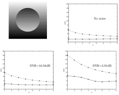
0 2 4 6 8 10 12 14 16 18 a error SNR=4.91dB
Figure 3.6: Comparison of the average error in the estimation of edge orientation (ex-pression (3.4.9)), for the disk image shown on the left, using the wavelet method (dashed line) versus the shearlet method (solid line), as a function of the scale a, for various SNRs (additive white Gaussian noise).