Scholarship@Western
Scholarship@Western
Electronic Thesis and Dissertation Repository
9-16-2013 12:00 AM
Resource Allocation in Uplink Long Term Evolution
Resource Allocation in Uplink Long Term Evolution
Aidin Reyhanimasoleh
The University of Western Ontario
Supervisor
Dr. Abdallah Shami
The University of Western Ontario
Graduate Program in Electrical and Computer Engineering
A thesis submitted in partial fulfillment of the requirements for the degree in Master of Engineering Science
© Aidin Reyhanimasoleh 2013
Follow this and additional works at: https://ir.lib.uwo.ca/etd
Part of the Systems and Communications Commons
Recommended Citation Recommended Citation
Reyhanimasoleh, Aidin, "Resource Allocation in Uplink Long Term Evolution" (2013). Electronic Thesis and Dissertation Repository. 1627.
https://ir.lib.uwo.ca/etd/1627
This Dissertation/Thesis is brought to you for free and open access by Scholarship@Western. It has been accepted for inclusion in Electronic Thesis and Dissertation Repository by an authorized administrator of
by
Aidin ReyhaniMasoleh
Graduate Program in Electrical and Computer Engineering
A thesis submitted in partial fulfillment
of the requirements for the degree of
Masters of Engineering Science
The School of Graduate and Postdoctoral Studies
The University of Western Ontario
London, Ontario, Canada
c
One of the crucial goals of future cellular systems is to minimize the transmission power while increasing the system performance. This thesis presents two channel-queue-aware schedul-ing schemes to allocate frequency channels among the active users in uplink LTE. Transmission power, packet delays and data rates are three of the most important criteria critically affecting the resource allocation designs. In the first algorithm, a resource allocation scheme is proposed which aims at minimizing system packet delays of three different data types (video, voice and data) and system transmission power at the same time. After formulating power consumption and packet delays, the four objective functions are collated into a single objective function by using the sum weighting method. propose a way to determine the weights of each objective function and solve the problem by using Binary Integer Programming (BIP). In the second work, we first develop an energy efficient rate adaptive scheduling approach that assigns sub-channels, transport block size, modulation and coding schemes as well as power to the active users in the uplink LTE. The objective function is to maximize the overall throughput of all the active users with respect to uplink standard restrictions and power threshold, which is adaptive at any given frame, per user. Another goal is to guarantee the users’ QoS requirements. In the proposed algorithm, we present an approach to reduce power consumption that adjusts the user maximum transmission power threshold according to the QoS requirement for each user. Sec-ondly, due to the high complexity of the adaptive algorithm, a less-complex heuristic algorithm is proposed. The numerical results prove that the adaptive and heuristic algorithms substan-tially improve the system performance in terms of transmission power while maintaining the demanding users’ QoS. In both of the proposed algorithms, the contiguity constraint, which makes the scheduling problem more complicated in uplink rather than downlink is considered.
I would like to first and foremost thank my supervisor, Dr. Abdallah Shami, not only for enthusiastically discussing my work with me, answering my questions and giving me good advice, but also for his patience and brilliant personality.
I would also like to thank my parents because without them I would not be here, my siblings (Arash, Azita and Aida) and my uncle (Hooshang) for all of their support. I cannot find a proper word to express my gratitude to them.
Thank you also to everyone in my Lab for all of your scientific and spiritual help.
Certificate of Examination ii
Acknowlegements ii
Abstract iii
List of Figures vii
List of Tables viii
Abbreviations ix
1 Introduction 1
1.1 Contributions . . . 3
1.2 Thesis Outline . . . 3
2 Long Term Evolution standard overview 4 2.1 System Performance Requirements . . . 4
2.2 Targets for the Long Term Evolution . . . 5
2.2.1 Maximum data rate and spectral efficiency per user . . . 5
2.2.2 Cell throughput and spectral efficiency . . . 5
2.2.3 Mobility . . . 5
2.2.4 User and control plane latency . . . 6
2.2.5 Other parameters . . . 6
2.3 Network Structure . . . 6
2.4 Protocol Architecture . . . 7
2.5 Physical Layer . . . 9
2.5.1 OFDM/OFDMA/SC-FDMA . . . 9
2.5.2 Radio Frame Structures . . . 10
2.5.3 Frequency Domain Organization . . . 12
2.6 Radio Resource Management . . . 14
2.6.1 Admission Control . . . 14
2.6.2 ARQ and HARQ . . . 15
2.6.3 Downlink Dynamic Scheduling and Link Adaptation . . . 16
2.6.4 Uplink Dynamic Scheduling and Link Adaptation . . . 18
2.6.5 Channel State Information . . . 19
3 Resource Allocation in Uplink LTE 23
3.1 Resource Allocation Definition . . . 23
3.2 Resource Allocation Modelling . . . 25
3.3 Search-based Scheduling Models . . . 27
3.3.1 Matrix-based Algorithms . . . 27
3.3.2 Pattern-based Algorithms . . . 28
3.4 The Size of Search Space . . . 30
3.4.1 Scenario 1: assignment of the whole PRBs among users . . . 30
3.4.2 Scenario 2: assignment of all or some PRBs among users . . . 31
3.5 Scheduling Strategy . . . 32
3.5.1 Channel-unaware . . . 32
3.5.2 Channel-aware/QoS-unaware . . . 34
3.5.3 Channel-aware/QoS-aware . . . 36
3.5.4 Power-aware . . . 38
3.6 Literature Review in Uplink LTE Scheduling . . . 38
4 Heterogeneous Delay-Power Resource Allocation in Uplink LTE 48 4.1 Queueing Theory Basics . . . 49
4.1.1 Little’s Law . . . 50
4.2 System Model . . . 50
4.2.1 Power criteria . . . 52
4.2.2 Packet delay criteria . . . 54
4.3 Problem Formulation . . . 55
4.3.1 Objective functions and variables . . . 55
4.3.2 Constraints . . . 56
4.4 Resource Allocation Solution . . . 57
4.5 Simulation and Numerical Results . . . 61
4.6 Chapter Summary . . . 65
5 Adaptive Power-efficient scheduler for LTE Uplink 66 5.1 Introduction . . . 66
5.2 System Model . . . 68
5.3 Adaptive Power-Efficient scheduling . . . 69
5.3.1 Delay analysis . . . 70
5.3.2 Adaptive MATP Design and The Objective Function . . . 71
5.4 Heuristic algorithm . . . 72
5.4.1 Complexity of the Heuristic Algorithm . . . 72
5.5 Numerical evaluation . . . 73
5.6 Chapter Summary . . . 75
6 Conclusion and Future Works 77 6.1 Future works . . . 78
A Source code of chapter 4 84
B Source code of chapter 5 89
Curriculum Vitae 94
2.1 Overall EPS architecture . . . 7
2.2 LTE Protocol Architecture . . . 8
2.3 Physical Structure in LTE . . . 11
2.4 Frame Structure type 2 . . . 12
2.5 Schematic of Downlink Scheduling. . . 17
2.6 The effect of contiguity constraint on FDPS . . . 19
2.7 Overall view of uplink scheduling in LTE . . . 20
3.1 TDPS/FDPS model . . . 27
3.2 Associated tree for given example.Thick line indicates the assignment . . . 40
3.3 A sample metric matrix . . . 40
3.4 Allocation difference between uplink and downlink . . . 41
3.5 Carrier by carrier method . . . 41
3.6 Bad example of carrier by carrier method . . . 42
3.7 Largest-metric-value-PRB-first method . . . 42
3.8 Bad example of largest-metric-value-PRB-first method . . . 43
3.9 Riding peaks method . . . 43
3.10 Bad example of riding peaks method . . . 44
3.11 The drawback of riding peaks method [1] . . . 45
3.12 PRB grouping method . . . 45
4.1 Queue model . . . 49
4.2 System schematic . . . 51
4.3 PDF of packet delay - one user in the cell . . . 62
4.4 PDF of packet delay - two users in the cell . . . 63
4.5 Average packet delay for different values of MTBS . . . 63
4.6 Average power delay for different values of MTBS . . . 64
4.7 Measure of complexity vs. MTBS . . . 64
4.8 Average power and packet delay vs. No. of users . . . 65
5.1 Average Delay . . . 74
5.2 Average Rates . . . 74
5.3 Normalized Average Power . . . 75
5.4 Normalized Average Time Consumptions . . . 75
2.1 downlink-uplink frame configuration in LTE . . . 12
2.2 Scalable Channel Bandwidth . . . 13
2.3 QCI Characteristics . . . 15
2.4 Supported MCS in LTE . . . 21
3.1 UE-PRB metric matrix . . . 28
3.2 A sample UE-PRB allocation . . . 31
3.3 Example of UE-PRB metric matrix . . . 39
4.1 Summary of notations . . . 52
4.2 Least-Squares Approximate Model Parameters for BLER=10% . . . 54
5.1 List of MCS Indices . . . 69
5.2 Heuristic Allocation . . . 72
5.3 Parameter settings of the uplink LTE model . . . 73
3GPP Third Generation Partnership Project
AMC Adaptive Modulation and Coding
BET Blind Equal Throughput
BIP Binary Integer Programming
BSR Buffer Status Reporting
CDMA Code Division Multiple Access
CQI Channel Quality Indicator
CSI Channel State Information
EDF Earliest Deadline First
EESM Exponential Effective SNR Mapping
FDPS Frequency Domain Packet Scheduling
FIFO First In First Out
GBR Guaranteed Bit Rate
HARQ Hybrid Automatic Repeat reQuest
LTE Long Term Evolution
LWDF Largest Weighted Delay First
MAC Medium Access Control
MCS Modulation and Coding Scheme
MIESM Mutual Information Effective SNR Mapping
MME Mobility Management Entity
MMSE Minimum Mean Square Error
MT Maximum Throughput
OFDM Orthogonal Frequency Division Multiplexing
PAPR Peak to Average Power Ratio
PF Proportional Fair
PRB Physical Resource Block
QoS Quality of Service
QSI Queue State Information
RBG Radio Bearer Group
RR Round Robin
SC-FDMA Single-Carrier Frequency Division Multiple Access
SDU Service Data Unit
SRS Sound Reference Signal
Introduction
The development of wireless communication systems has been non-stop in the past decade. First generation cellular networks (1G) were analog-based and limited to voice services only. The first 1G cellular mobile communication system was the Advanced Mobile Phone System (AMPS) that was developed by Bell Labs in the late 1970s [2] and used commercially in the United States in 1983. While these 1G systems give reasonably good voice quality, they offer low spectral efficiency.
This is why the evolution toward 2G was necessary to overcome the drawbacks of 1G technology. The main design objective in Second Generation (2G) cellular networks was to increase voice quality. The second generation of cellular systems, first deployed in the early 1990s, was based on digital communications. The two main categories of 2G cellular systems are GSM (Global System for Mobile Communications) and CDMA (Code Division Multiple Access). The most significant features of GSM that differ from 1G are: (1) using digital cel-lular technology and (2) exploiting the Time Division Multiple Access (TDMA) transmission method. In the US, 2G cellular networks use direct-sequence CDMA technology with phase shift-keyed modulation and coding. There are three sophisticated versions of GSM [3]:
• High Speed Circuit Switched Data (HSCSD): which yields higher data rates for circuit-switched services as a result of a changing coding scheme and using multiple time slots.
• General Packet Radio Service (GPRS): which had efficient support for non real time packet data traffic. Maximum peak data rates of GPRS are 140 Kbps.
• Enhanced Data rates for Global Evolution (EDGE): which has the maximum data rate 384 Kbps by employing a high-level modulation and coding scheme.
Further progress on the GSM-based and CDMA-based systems have been handled under 3GPP and 3GPP2, respectively. 3GPP introduced the Universal Mobile Telecommunications System (UMTS) as the first global third generation cellular network. The main components of this system are the UMTS Terrestrial Radio Access Network (UTRAN) where Wideband Code Division Multiple Access (WCDMA) radio technology is employed due to its 5 MHz band-width, and the GSM/EDGE radio access network based on GSM-enhanced data rates [4].The third generation continues its improvements and so 3GPP has introduced High-Speed Down-link Packet Access (HSDPA) that resulted in higher speed data services in 2001. Then in 2005, High-Speed Uplink Packet Access (HSUPA) was introduced. The combination of HSDPA and HSUPA is called HSPA [5]. The last evolution of the HSPA category was the HSPA+, which has features such as Multiple Input/Multiple Output (MIMO) antenna capability and 16 QAM (uplink)/64 QAM (downlink) modulation. Due to improvements in the radio access network for packets, HSPA+will allow speeds of 11 Mbps and 42 Mbps for uplink and downlink, re-spectively. One of the new concepts in HSPA+ is combining multiple cells into one with a technique known as Dual-Cell HSDPA.
4G networks are sophisticated IP solutions that provide voice, data, and video to mobile users. They offer significantly improved data rates compared with previous generations of wireless technology. Faster wireless connections enable wireless devices to support higher level data services, such as streamed audio and video, video conferencing, gaming and naviga-tion.
specifica-tions of LTE equipment were released (Release 8) at the end of 2008. However, some small enhancements were introduced in Release 9, a release that was functionally finalized in De-cember 2009.
1.1
Contributions
The two main contributions of this thesis are:
In the first algorithm, a resource allocation method which includes packet delays and trans-mitted power consumption simultaneously is proposed. In this work, after formulating the objective functions (packet delays and power consumption) the scheduler uses the weighted sum method to convert multiple objective functions into a single one. Finally a binary integer optimization method is employed to solve the scheduling problem.
In the second algorithm, a power threshold mechanism is introduced. This power threshold mechanism adapts power threshold for each frame based on the user’s Quality of Service (QoS) requirements. The required QoS is power outage delay which implies that probability of out-age delay should be less than 2%. In other words, for users who are demanding high QoS, the scheduler increase their power threshold to meet their QoS requirements and the scheduler for users who have low traffic loads decrease their power threshold to save power.
1.2
Thesis Outline
Long Term Evolution standard overview
This chapter provides preliminary system information on different specifications of the LTE system. At first, system performance requirements and targets for LTE are presented. The discussion is followed by the network structure and protocol architecture of LTE. Then some aspects of the physical layer in LTE are clarified . Finally, the chapter concludes with the radio resource management concept in LTE with a focus on the scheduling process.
2.1
System Performance Requirements
Before standardization of LTE, 3GPP highlighted the most basic requirements for the LTE:
• The LTE system should be packet switched optimized
• A true global roaming technology with the inter system mobility with GSM, WCDMA and CDMA2000
• Reduced latency with radio round trip time below 10 ms and access time below 300 ms
• Scalable bandwidth from 1.4 MHz to 20 MHz
• Increased spectral efficiency and user data rates
• Simple protocol architecture
• Increased cell-edge bit-rate
2.2
Targets for the Long Term Evolution
The following list is some of the important targets of LTE.
2.2.1
Maximum data rate and spectral e
ffi
ciency per user
The most important parameter by which the different standards compare with each other is the achievable maximum per-user data rate. This peak data rate depends on used bandwidth and the number of transmitter and receiver antennas in MIMO systems. The maximum data rates for downlink and uplink in the LTE system were set at 100 Mbps and 50 Mbps respectively by using a 20 MHz bandwidth, with the assumption of two receiver antennas and one transmit-ter antenna for each transmit-terminal. Hence maximum spectral efficiencies of 5 and 2.5 bps/Hz are achieved in downlink and uplink LTE, respectively.
2.2.2
Cell throughput and spectral e
ffi
ciency
Performance at cell level critically depends on the number of cell sites that a network operator needs and therefore determine the main cost of developing a new system. To access the per-formance at the cell level, 2 metrics are defined: (1) average cell spectral efficiency which is around 1.6-2.1 bps/Hz/cell, (2) cell-edge user spectral efficiency (which used to assess 5% of user throughput) is about 0.04-0.06 bps/Hz/user.
2.2.3
Mobility
2.2.4
User and control plane latency
The average time between the sending of a data packet and the reception of a physical layer Acknowledgement (ACK) determines user plane latency (by considering typical HARQ re-transmission rates). Simplicity, the round trip time is twice of user plane latency. Reduction of call set-up delay is one of the significant requirements of LTE system. This results in both good user satisfaction and more importantly affects the battery life of terminals. In other words, con-trol plane latency is the amount of time delay between the sending of a command message or the initiation of a service request to when the command begins to process or the service begins to operate.
2.2.5
Other parameters
Besides the system performance aspects, a number of other criteria are important for network operators. These include reduced deployment cost, bandwidth flexibility, compatibility with other radio access technologies, and lower power consumption terminals [7].
2.3
Network Structure
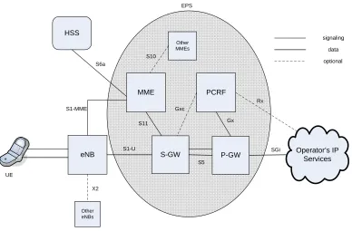
and (3) Packet Data Network Gateway (PDN-GW) which is responsible for IP address alloca-tion for the UE, as well as QoS enforcement for Guaranteed Bit Rate (GBR) bearers. Note that E-UTRAN and EPC together constitute the Evolved Packet System (EPS). Figure 2.1 shows the overall EPS architecture.
eNB
Other eNBs
Operator’s IP Services
S-GW P-GW
MME PCRF
Other MMEs
HSS
X2
S1-U
S5
SGi Rx Gxc
Gx S10
S11 S6a
S1-MME
EPS
signaling data optional
UE
Figure 2.1: Overall EPS architecture
2.4
Protocol Architecture
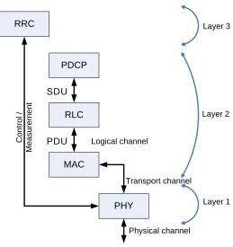
sub-layer of the link layer i.e. Radio Link Control (RLC). RLC is responsible for reassembly of SDUs into Protocol Data Units (PDUs). This reassembly can be either segmentation of one SDU into several PDUs or, concatenation of several SDUs to form one PDU due to the transmission data rate. The lowest sub-layer of the link layer is the Medium Access Control (MAC) sub-layer that handles Hybrid Automatic Repeated reQuest (HARQ) functionality and scheduling problems. The Physical (PHY) layer performs all of the tasks regarding the trans-mission of actual data to air interface such as modulation and coding. Figure 2.2 depicts the protocol architecture of LTE. As shown in the Figure the channel between air and PHY layer is the physical channel, the channel between PHY layer and the MAC sub-layer is the transport channel and between the MAC and the RLC sub-layers is the logical channel.
RRC
PDCP
RLC
MAC
PHY
Layer 3
Layer 2
Layer 1
Physical channel Transport channel Logical channel
Control
/
Measurement
SDU
PDU
2.5
Physical Layer
In this section, different features and specifications of the physical layer in LTE are briefly investigated. A comprehensive investigation of this concept by itself needs several hundred pages to cover them. For the sake of brevity, this section just explores the key concepts of the physical layer.
2.5.1
OFDM
/
OFDMA
/
SC-FDMA
• High spectral efficiency, which is also called bandwidth efficiency. This term means that more data can be transmitted in presence of the noise in a given bandwidth during a fixed time interval. The unit of spectral efficiency is bits per second per Hertz (b/s/Hz).
• Robustness to multi path delay spread as a result of long symbol time and guard interval
• Flexible utilization of frequency spectrum
• Low-complexity receivers, by exploiting frequency-domain equalization
• Effectiveness against Channel Distortion due to utilization narrow bandwidth
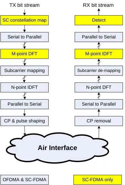
However, despite its many advantages, OFDMA has certain drawbacks such as high sensitivity to frequency offset and high peak-to-average power ratio (PAPR) due to in-phase addition of subcarriers. The second one plays an important role in uplink direction where transmitters are cell phones with limited power storage. 3GPP selected Single Carrier FDMA (SC-FDMA) as multiple access method of uplink in LTE because this scheme possesses the same advan-tages of OFDMA while experiencing lower PAPR. The adoption of SC-FDMA enhances the power consumption efficiency of the cell phone batteries, hence prolonging their lifetimes. SC-FDMA exhibits 3-6 dB less PAPR than OFDMA. The main reason for the selection of SC-FDMA among other PAPR reduction methods is the similarity of SC-FDMA to OFDMA in implementation structure. Figure 2.3 illustrates the structure of the physical layer in LTE. As can be seen, the only difference between SC-FDMA and OFDMA is the presence of a DFT and an IDFT block in the transmitter and receiver, respectively. That is why that SC-FDMA is also known as DFT pre-coded OFDMA.
2.5.2
Radio Frame Structures
SC constellation map
Serial to Parallel
Subcarrier mapping
N-point IDFT
Parallel to Serial
CP & pulse shaping M-point DFT
Detect
Parallel to Serial
Subcarrier de-mapping
N-point DFT
Serial to Parallel
CP removal M-point IDFT
TX bit stream RX bit stream
Air Interface
SC-FDMA only OFDMA & SC-FDMA
Figure 2.3: Physical Structure in LTE
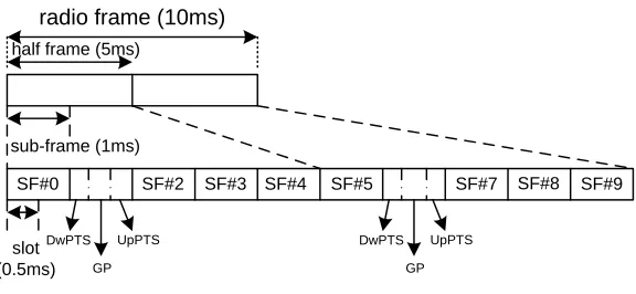
processing, like scheduling. Each sub-frame consists of two time slots, which are each 0.5ms long. Each time slot depends on the duration of Cyclic Prefix (CP), which has 6 or 7 OFDM/ SC-FDMA symbols. Frame structure Type 2 is only applicable to TDD, which utilizes the same frequency band in uplink and downlink and shares frames in time domain. The structure of each Type 2 frame is identical to Type 1. The only difference is the existence of one or two special sub-frames that help switching between uplink and downlink transmissions. These special sub-frames have three special fields: the downlink pilot timeslot (DwPTS), the guard period (GP) and the uplink pilot timeslot (UpPTS). The duration of these three fields is equal to one sub-frame. Figure 2.4 shows the Type 2 frame structure of LTE.
radio frame (10ms)
half frame (5ms)
SF#0 SF#2 SF#3 SF#4 SF#5 SF#7 SF#8 SF#9 sub-frame (1ms)
slot (0.5ms)
DwPTS UpPTS
GP
DwPTS UpPTS
GP
Figure 2.4: Frame Structure type 2
a special sub-frame for the switching purpose. Note the sub-frame 0 and sub-frame 5 in all configurations are for downlink. Sub-frames immediately following the special sub-frame (i.e., sub-frame 2 in all configurations and sub-frame 7 in 5ms periodicity) are always reserved for the UL transmission.
Configuration DL to UL sub-frame number
# switch priority 1 2 3 4 5 6 7 8 9 10 0 5ms D S U U U D S U U U 1 5ms D S U U D D S U U D 2 5ms D S U D D D S U D D 3 10ms D S U U U D D D D D 4 10ms D S U U D D D D D D 5 10ms D S U D D D D D D D 6 5ms D S U U U D S U U D
Table 2.1: downlink-uplink frame configuration in LTE
2.5.3
Frequency Domain Organization
Resource Element is one 15 kHz subcarrier by one symbol. Resource Elements aggregate into Resource Blocks. A Resource Block has dimensions of subcarriers by symbols. Twelve consecutive subcarriers in the frequency domain and six or seven symbols in the time domain form each Resource Block. As noted, the number of symbols depends on the Cyclic Prefix (CP) in use. When a normal CP is used, the Resource Block contains seven symbols. When an extended CP is used, the Resource Block contains six symbols. A delay spread that exceeds the normal CP length indicates the use of extended CP. Various channel bandwidths that may be considered for LTE deployment are shown in Table 2.2.
Channel Bandwidth (MHz) 1.4 3 5 10 15 20 No. of Sub-carriers 73 181 301 601 901 1201 FFT Size 128 256 512 1024 1536 2048 Sampling Rate (MHz) 1.92 3.84 7.68 15.36 23.04 30.72 No. of PRBs 6 15 25 50 75 100
Table 2.2: Scalable Channel Bandwidth UL/DL resource grid definitions are summarized as:
• Resource Element (RE): One element in the time/frequency resource grid. One sub-carrier in one OFDM/SC-FDMA symbol for DL/UL. Often used for Control channel resource assignment.
• Physical Resource Block (PRB): 12 consecutive sub-carriers (180 kHz) over the duration of one slot, which is the minimum scheduling size for DL/UL data channels.
• Resource Block Group (RBG): Group of Resource Blocks where the size of RBG de-pends on the system bandwidth in the cell.
• Resource Element Group (REG): Groups of Resource Elements to carry control infor-mation. The size of REG is four or six REs depending on the number of reference signals per symbol, cyclic prefix length.
2.6
Radio Resource Management
The aim of RRM is to maximize the radio resource efficiency by utilization of the adaptation techniques and satisfying the configured users’ Quality of Services. There are two categories of RRM algorithms: (1) semi-dynamic category; which are mainly executed during the setup of new data flows and (2) fast dynamic category named such since every action is carried out at each sub-frame (1 ms). The semi-dynamic category consists of three algorithms: QoS man-agement, admission control, and semi-persistent scheduling, all of which are in Layer 3. The fast dynamic category includes Hybrid Adaptive Repeat and Request (HARQ) management, dynamic packet scheduling, and link adaptation in Layer 2 as well as the Channel Quality Indicator (CQI) manager, and power control in Layer 1.
2.6.1
Admission Control
QCI # Type Priority Packet delay budget Packet loss rate Example services 1 GBR 2 100ms 10−2 Conversational voice
2 GBR 4 150ms 10−3 Conversational video
3 GBR 5 300ms 10−6 Buffered streaming 4 GBR 3 50ms 10−3 Real time gaming
5 non-GBR 1 100ms 10−6 IMS signalling
6 non-GBR 7 100ms 10−3 Live streaming
7 non-GBR 6 300ms 10−6 Buffered streaming, email,
8 non-GBR 8 300ms 10−6 browsing, file download,
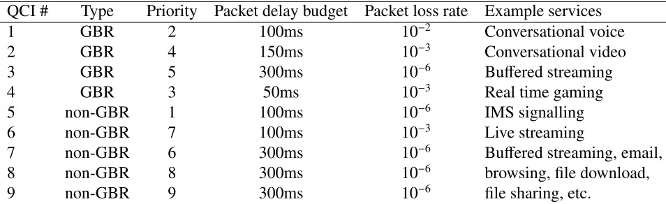
9 non-GBR 9 300ms 10−6 file sharing, etc. Table 2.3: QCI Characteristics
In uplink, per bearer, there is another QoS parameter named prioritized bit rate (PBR). The aim of PBR is to avoid uplink scheduling starvation problems for UEs with multiple bearers. PBR differs from GBR and can also be defined for non-GBR bearers. The uplink rate control mechanism ensures that the UE serves at first the radio bearers in decreasing priority order up to their PBR, and then the radio bearers in decreasing priority order for the remaining resources.
2.6.2
ARQ and HARQ
As in any communication system, there are data transmission errors, which can be due to noise and interference. Most of the protocols are not able to correct errors in the data packets. To solve this problem, complementary mechanisms are required. An approach is to deploy backward error correction (aka Automatic Repeat Request). In ARQ, the receiver informs the transmitter whether a data packet was received correctly or not. If the reception is erroneous, the transmission is repeated. Although this mechanism is simple and significantly efficient, there are some drawbacks as listed below:
• ARQ results in delay in transmission of data packets and this delay is grown out of feedback response and retransmission if data are transmitted incorrectly.
• ARQ is efficient if the average packet error rate is reasonably small.
ARQ is not optimal because it throws away the information in the erroneous packet. A su-perior method is that the receiver stores and exploits all of the past received information. Even if the received data from the first transmission is not enough for successful decoding, it can still be helpful if combined with the second transmission. This scheme is called Hy-brid ARQ (HARQ). In general, HARQ schemes can be categorized as adaptive-synchronous, non-adaptive-synchronous, adaptive-asynchronous and non-adaptive-asynchronous. In a syn-chronous HARQ schemes, the retransmission time relative to the first transmission is specified and so there is no need for an information signal, for example a HARQ process number. How-ever, in an asynchronous HARQ scheme, the retransmissions can happen at any time after the first transmission, which causes asynchronous HARQ to need extra signalling to transmit the HARQ process number to the receiver. As a result, synchronous HARQ schemes have the ad-vantage of decreasing the signalling load and the disadad-vantage of less flexibility in scheduling compared to asynchronous HARQ schemes. In an adaptive HARQ scheme, the retransmissions can be employed either the same or with another modulation and coding scheme and resource allocation in the frequency domain relative to initial transmission. The changes in transmission attributes arises from variation in the channel condition. This means this scheme needs addi-tional signalling. By contrast, in the non-adaptive HARQ scheme, the retransmissions do not need the explicit signalling of new transmission attributes, since retransmissions are executed either the same as the initial transmission or with new attributes, which is determined accord-ing to a predefined regulation. In summary, adaptive schemes have more schedulaccord-ing gain at the expense of increased signalling overhead. In LTE, asynchronous adaptive HARQ is used for the downlink, and synchronous HARQ for the uplink. In the uplink, the retransmissions may be either adaptive or non-adaptive depending on whether new signalling of the transmission attributes is provided.
2.6.3
Downlink Dynamic Scheduling and Link Adaptation
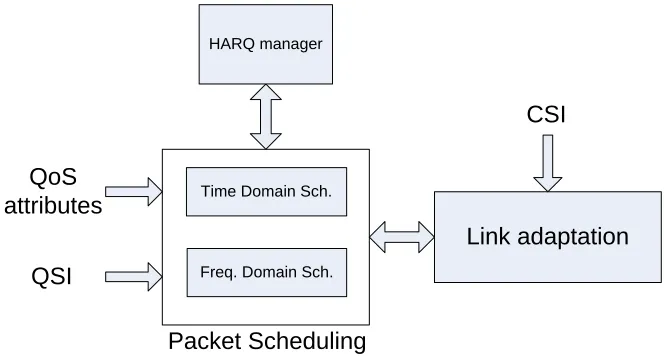
transmission parameters such as modulation and coding schemes, which is called link adapta-tion. In other words, the purpose of packet scheduling is to maximize the cell throughput, while the minimum QoS requirements for the EPS bearers are met and remain adequate resources for best-effort bearers. The best-effort bearers have no strict QoS requirements. Figure 2.5 depicts the general schematic of downlink scheduling.
Time Domain Sch.
Freq. Domain Sch.
QoS attributes
QSI
Link adaptation
HARQ manager
CSI
Packet Scheduling
Figure 2.5: Schematic of Downlink Scheduling.
the frequency domain scheduler and then the frequency domain scheduler assigns PRBs to the selected users. The complexity of this method is much lower than fully time/frequency domain scheduler, while it has almost the same performance. If HARQ retransmissions are included in scheduling, Time Domain Scheduler (TDS) passed all of the users that have pending HARQ retransmission to FDPS. Two scenarios exists for HARQ-aware FDPS. In scenario #1, in the first step, Nharq PRBs are reserved for all of the users with pending HARQ retransmissions. In the second step, all of the remaining PRBs are assigned to the users with new data packets based on FDPS metric value (this metric depends on many parameters such as channel gain and so on) and in the third step, the remaining PRBs are allocated to HARQ retransmissions. Scenario #2 is the same as #1 but exchanges the order of the second and third steps. In both scenarios, it is assumed the number of required PRBs for retransmission is the same as the initial transmission. It is obvious that the latter scenario gives the higher priority to the HARQ retransmission relative to the former scenario.
2.6.4
Uplink Dynamic Scheduling and Link Adaptation
In uplink LTE, there are some special features that make the scheduling in uplink different from that in downlink. The three main differences are listed as follows:
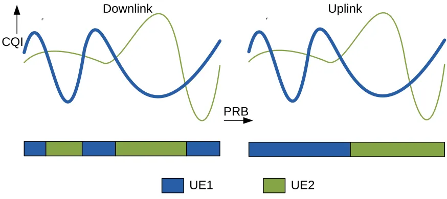
1. The first and the most important distinction is PRB contiguity allocation constraint. Con-tiguity constraint implies all of the multiple PRBs assigned to a certain user have to be adjacent to each other. This limitation is derived from SC-FDMA. Figure 2.6 illustrates the comparison of uplink/downlink FDPS with/without contiguity constraint. This con-straint limits both frequency and multi-user diversity.
2. In uplink, data transmitters are UEs that have limited transmitter power compared to base stations in downlink. On the other hand, UEs tend to decrease power consumption to prolong the battery life time of UEs. In summary, uplink has less power budget relative to downlink.
CQI
PRB
Downlink Uplink
UE1 UE2
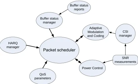
Figure 2.6: The effect of contiguity constraint on FDPS Figure 2.7 shows the overall view of uplink scheduling in LTE.
High efficient packet scheduling and link adaptation are strongly related to two main cate-gories of information, which are Channel State Information (CSI) and Queue State Information (QSI).
2.6.5
Channel State Information
CSI is applied to AMC block to affect selection of MCS and Scheduling block to perform FDPS. CSI is calculated based on the SNR measurements of Sound Reference Signals (SRSs) in uplink. Allocation of SRS resources among the users is one of the RRM functions in up-link. The purpose of allocation is to update channel state information. There is a compromise between measurement precision and SRS bandwidth in such a way that, by decreasing the SRS bandwidth, the measurement becomes more accurate. However, to know of the entire bandwidth, several SRS transmissions are required.
2.6.6
Adaptive Modulation and Coding
Buffer status reports
HARQ manager
QoS parameters
Adaptive Modulation and Coding
Power Control
SNR measurements
CSI manager Buffer status
manager
Figure 2.7: Overall view of uplink scheduling in LTE
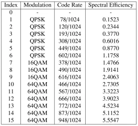
manager and the packet scheduler. The second task is to select the most efficient MCS for a certain user once the allocated bandwidth for the corresponding user is specified. By using a proper AMC, obviously the spectral efficiency of a wireless system is increased. In practice, AMC is performed by employing AMC mapping tables. These tables return the MCS and the corresponding Transport Block Size based on SNR value and the given Block Error Rate (BLER). At any TTI, AMC selects the MCS that maximizes the expected transport block size (T). Expected transport block size is a function of TBS and Block Error Probability (BLEP), which infers the probability of the erroneous transmitted block as shown in the following:
commands and (2) fast AMC; in which AMC is performed at each TTI. Clearly, the fast AMC leads to better gain compared to the slow one. That is why all of the schedulers select fast AMC as a default. All of the supported MCS in LTE and their characteristics are illustrated in Table 2.4.
Index Modulation Code Rate Spectral Efficiency
0 - -
-1 QPSK 78/1024 0.1523 2 QPSK 120/1024 0.2344 3 QPSK 193/1024 0.3770 4 QPSK 308/1024 0.6016 5 QPSK 449/1024 0.8770 6 QPSK 602/1024 1.1758 7 16QAM 378/1024 1.4766 8 16QAM 490/1024 1.9141 9 16QAM 616/1024 2.4063 10 64QAM 466/1024 2.7305 11 64QAM 567/1024 3.3223 12 64QAM 666/1024 3.9023 13 64QAM 772/1024 4.5234 14 64QAM 873/1024 5.1152 15 64QAM 948/1024 5.5547
Table 2.4: Supported MCS in LTE
2.6.7
Power Control
The main goal of power control is to limit inter-cell interference while considering QoS require-ments and to minimize UE power consumptions to prolong the battery life of users. Based on [10], transmit power of each UE can be calculated by the following equation:
P=min{Pmax,P0+10log10N+αL+ ∆MCS + f(∆i)} (2.2)
wherePmaxis the maximum user transmission power,N is the number of allocated PRB at a given TTI,P0 andαare power control parameters, Lis the downlink path-loss measured in
the UE and is a function of distance, path loss, shadowing and antenna gain. ∆MCS is a cell
correction. It is noticed that α is cell-dependent and takes the value zero or 0.4 to 1.0 with the step of 0.1, whileP0 can either be cell- or user- dependent. As a result, the task of power
control is to (1) modify the transmission power of users with respect to radio propagation channel, including path loss, shadowing and fast fading and (2) overcome interference from inter-cell and intra-cell users.
2.6.8
Bu
ff
er Status Reporting
In LTE, Buffer Status Reporting (BSR) includes the buffer size of several Radio Bearer Groups (RBGs) for each user. This scheme offers relatively low signalling load and high flexibility in scheduling. BSR consists of at most four different RBGs to report. The mapping of each radio bearer to the corresponding RBG is performed based on vendor-specific mapping tables by considering the radio bearer QoS. The buffer size of each RBG represents the amount of data relevant to radio bearers of a certain RBG. There are two formats of BSR in LTE.
• Short BSR format: in this format, a certain user just sends the buffer size of one RBG and the identifier of the transmitted RBG.
• Long BSR format: all of the four buffer sizes of each user are transmitted.
Resource Allocation in Uplink LTE
This chapter provides more detailed discussion of the resource allocation problem. This chapter starts by the defining resource allocation problem and modelling. Then, two types of search-space scheduling models, as well as the largeness of the search search-space, are explained. Different scheduling strategies are then investigated. Finally, a literature review of existing works re-garding resource allocation in uplink LTE has been provided.
3.1
Resource Allocation Definition
In wireless shared bandwidth networks, resource allocation is defined as allocation of a portion of bandwidth and power to different users to improve network performance. In uplink LTE, since different MCSs can be supported, the most efficient MCS should be assigned to the user in addition to physical resource blocks and power. All of the scheduling tasks are performed in the MAC sub-layer located in the eNB. Because of SC-FDMA characteristics, channel variation in space, time and frequency per user can be utilized by the scheduler. A good scheduler should contain two attributes at the same time. The first one is to satisfy the QoS requirements of users and the second one is to increase the efficiency of resources allocated to the users. In general, the scheduler should take into account some or all of the following factors simultaneously as follows:
• CSI: provide the channel quality information between users and eNB over different PRBs. The information is used by the scheduler to efficiently assign the PRBs to users.
• QSI: with knowledge of users’ QSI, the scheduler assigns more PRBs to the users which have more available data in their buffers. Also the scheduler ensures not to assign trans-port block sizes more than the available queue size of each user.
• QoS requirements: the scheduler must guarantee to provide the user’s QoS. In the so-phisticated schedulers, each user has different traffic types which have their own QoS (such as average delay, guaranteed bit rate and packet error rate).
• HARQ retransmission: the scheduler decides which PRBs should be reserved for HARQ retransmissions and which ones for new transmissions.
• Maximum No. of users: in some of the scheduling algorithms, a predefined maximum No. of users is allowed to be served at each TTI.
• History of user rates: this history can be deployed to consider the fairness of the users. In the channel-aware scheduling, the users close to the edge of the cell experience pretty bad channel quality rather than users close to the eNB and so have a lower chance to take the bandwidth. To avoid this unfairness in taking sub-channels, the history of user rates are included in the scheduling.
• User priority: some users have more priority than others. This priority should be consid-ered in the scheduling problem.
• Allocation constraint: as with other shared bandwidth resource allocation schemes, each PRB can be assigned to at most one user.
• Contiguity constraint: SC-FDMA imposes contiguity constraints in the uplink schedul-ing. According to this limitation, all of the allocated PRBs to each user have to be adjacent to each other. This restriction makes the scheduling problem more complicated in uplink compared to downlink.
• Complexity: packet scheduling decisions are made in sub-frame duration (1ms). Thus the scheduling scheme should have low complexity to limit processing time and memory usage.
The scheduling algorithm takes into account some of or all of the above factors to maximize or minimize a desired aim. The most important objectives are listed as follows:
• Maximization of the overall cell throughput: one of the most important performance indicators in effective utilization of radio interface in any cellular network is the actual throughput or spectral efficiency (expressed in bit/s/Hz). Actual throughput refers to data rate without including HARQ retransmissions. The overall cell throughput can be calculated as a summation of active user throughput of the cell.
• Maximization of fairness: a blind maximization of the overall cell throughput leads to an unfair resource sharing among users. If the scheduler just focuses on spectral efficiency, the users with bad channel quality (such as cell-edge users) can have less opportunity to take allocation resources.
• Minimization of power consumption: in uplink, power consumption is an important fea-ture which should be considered in scheduling to prolong the battery life time of cell-phones. Power consumption in uplink is more important than that in downlink because transmitter units in uplink are cell-phones fed from limited energy batteries while in downlink the transmitter units are eNBs with unlimited energy suppliers.
• QoS provisioning: some schedulers just emphasize the satisfaction of users’ QoS re-quirements.
3.2
Resource Allocation Modelling
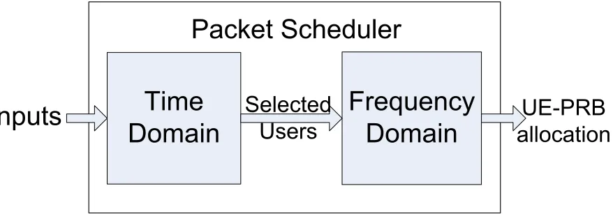
with the optimal solution can be complicated. By using this model, each scheduling scheme includes two stages:
1. Determination of the objective function: objective function is a mathematical formula which maps a satisfaction level of the system performance to a quantitative value. Based on the scheduler’s strategy, the desired system performance can include one or a combi-nation of the mentioned objectives in Section 3.1. The satisfaction level of the system is related to the satisfaction level of the available users in the cell. Hereafter, quantitative value of the user’s satisfaction level will be known as user utility and denotes asUi and the quantitative value of the system’s satisfaction level will be known as system utility and denotes asUsys. Apparently, Usys is a function of Ui and the simplest form of this function is summation.
Usys = K
X
i=1
Ui (3.1)
Depending on the parameters which are included in the utility function, system utility values differ in each TTI.
2. Determination of the search based allocation scheme: the scheduler runs an algorithm which searches among all of the UE-PRB allocation patterns until it comes up with the pattern which best optimizes the defined system utility function. The scheduler should implement search based allocation algorithms once per sub-frame (1ms). Hence, devis-ing a low complex algorithm that approximates to that of the optimal algorithm is of great importance. According to the selected performance strategy, the optimization problem can be a minimization algorithm (e.g. packet delay or packet loss rate) or maximization one (like system throughput or fairness among users).
The simplified version of this model is that it bypasses the first block. In other words, all of the active users in the cell passed into the FDPS block.
Figure 3.1: TDPS/FDPS model
3.3
Search-based Scheduling Models
As noted, the solution in packet scheduling is to find the best UE-PRB pattern to maximize or minimize system performance utility. Almost all of the search based algorithms in uplink LTE can be classified as one the following models.
3.3.1
Matrix-based Algorithms
In this model, the scheduler forms a matrix. The matrix hasKrows according to the number of active users in the cell andMcolumns relevant to the number of PRBs which can be scheduled. Each element of this matrix represents a metric value that is achieved from the utility function whereMi,mdenotes the metric value for useriand PRBm. Table 3.1 shows the UE-PRB metric matrix. The allocation algorithms select the maximum metric value in the matrix and assign the corresponding PRB to the associated user by keeping in mind the defined standard constraint (allocation and contiguity constraints).
PRB1 PRB2 . . . PRBM
U E1 M1,1 M1,2 . . . M1,M
U E1 M2,1 M2,2 M2,M
... ... ...
U EK MK,1 MK,2 . . . MK,M
Table 3.1: UE-PRB metric matrix
the importance of users based on the selected policy and then select the set of users with maximum metric to pass into the FDPS block. Therefore, in this model, two utility functions and accordingly two metrics should be defined.
3.3.2
Pattern-based Algorithms
In this model, the scheduler forms one binary matrix corresponding to all of the feasible PRB allocation patterns and one cost or reward vector based on the selected utility function. The binary matrix, which is named the constraint matrix and shown byA, has Mrows regarding the number of available PRBs andC×Kcolumns corresponding the number of feasible allocation patterns for each user (C) and number of users (K). Each entry of this matrix has a binary value which indicates whether a certain PRB is assigned to the associated user or not. The idea can be described by a simple example. Suppose that there are four PRBs and two users (M = 4,K = 2). For a given user, by ignoring the PRB allocation of the other users, in this case there are a few feasible allocation patterns that can be allocated to the given user. Now for the particular useri, the constraint matrix (Ai) will be shown as:
Ai =
0 1 0 0 0 1 0 0 1 0 1 0 0 1 0 0 1 1 0 1 1 1 0 0 0 1 0 0 1 1 1 1 1 0 0 0 0 1 0 0 1 0 1 1
columns for each user is
C= 1+
M
X
m=1
(M−(m−1))= 1 2M
2+ 1
2M+1 (3.3) The system constraint matrix (A) is two replicas of theAi because there are two users in the system and can be shown as:
A=
user 1
z }| {
0 1 0 0 0 1 0 0 1 0 1 0 0 1 0 0 1 1 0 1 1 1 0 0 0 1 0 0 1 1 1 1 1 0 0 0 0 1 0 0 1 0 1 1
user 2
z }| {
0 1 0 0 0 1 0 0 1 0 1 0 0 1 0 0 1 1 0 1 1 1 0 0 0 1 0 0 1 1 1 1 1 0 0 0 0 1 0 0 1 0 1 1
(3.4)
It is worthwhile to mention three important points with respect to the constraint matrix (A): (1) each pattern in this matrix contains the contiguity constraint and (2) for each user just one of the patterns fromAmhas to be selected as well as (3) each PRB should be allocated to at most one user. The cost or reward vector (R) is calculated based on the selected utility function and scheduling strategy for each column of matrix A. For each column of matrixA, the allocated PRBs for the associated user are determined and the utility function can be calculated according to the known utility function. Therefore, the reward vector hasC×Kdifferent elements. These search-based algorithms use set partitioning approach to solve the scheduling problem. The reward vector for the given example is shown as follows:
R=
R1,1 · · · R1,C R2,1 · · · R2,C
3.4
The Size of Search Space
In this section, the number of feasible solutions to allocate M PRBs among K users is calcu-lated. This calculation just considers the FDPS search space. Two scenarios can be regarded in computation of search space. This section specifies how large the search space of scheduling can be in the allocation problem. In the following parts of this section, it is assumed that there areK active users and M available PRBs. In practic e, the set of allowed value of M is given as{6,15,25,50,75,100}based on Table 2.2 concerning the selected bandwidth.
3.4.1
Scenario 1: assignment of the whole PRBs among users
In this scenario, it is assumed that all of the PRBs are assigned to the users and there is no unallocated PRB after scheduling. At first we selectµusers out ofKand distribute theMPRBs among these users. Due to the contiguity constraint in uplink LTE, we should share M PRBs intoµordered set wherein each set has mi adjacent PRB, which is assigned to useri. Hence, we should calculate the number of different combinations that satisfiesM =m1+m1+. . .+mµ.
In combination theory, this problem has
M−1
µ−1
different solutions [11] and there are µ permutations ofK patterns to selectµusers out ofK total users by considering the sequence. Therefore, there are
M−1
µ−1
P(K, µ) possible PRB allocations whichµusers employ the M
PRB. Adding all the allowable numbers of the users, the search space will be
K
X
µ=1
M−1
µ−1
P(K, µ)=
K
X
µ=1
K µ µ!
M−1
µ−1
(3.6) As a practical case, assuming of 25 PRBs (M = 25) and 10 active users (K = 10), the search space has 5.26 ×10¹² possible allocation patterns and the scheduler should traverse among
them and choose the most efficient one. Assume that checking for one possible solution takes 1×10⁻⁹ seconds. The running time of a complete search is about 5.26×10³seconds and this
PRB allocation Set of assigned Set of assigned Relevant column inA Relevant column inA
No. PRBs for user 1 PRBs for user 2 matrix for user 1 matrix for user 2
1 ∅ {1,2,3,4} 1 22
2 {1} {2,3,4} 2 21
3 {1,2} {3,4} 6 19
4 {1,2,3} {4} 9 16
5 {1,2,3,4} ∅ 11 12
6 {2,3,4} {1} 10 13
7 {3,4} {1,2} 8 17
8 {4} {1,2,3} 5 20
Table 3.2: A sample UE-PRB allocation
3.4.2
Scenario 2: assignment of all or some PRBs among users
In this scenario, it is assumed that either all or some of the PRBs are assigned to the users and it is likely that, after scheduling, some of the PRBs are not allocated to the users. Again we assumeµout of K users are chosen for scheduling. The set of allocated PRBs for each of µ user is shown as ai where i is the index of the user. We arrange these sets in order of PRB number and define starting the PRB number (ais) and finishing (aif) PRB number for each of the differentµsets. Due to the contiguity constraint in uplink, we have
1≤a1s ≤ a1f <a2s ≤ a2f . . . <asµ ≤aµf ≤ M (3.7) as noted Mis the number of available PRBs. By a little manipulation of Equation 3.7:
1≤a1s <a1f +1< as2+1<a2f +2. . . <asµ+µ−1< aµf +µ≤ M+µ (3.8) Thus, the number of choices of µ sets of contiguous PRBs is equal to the number of 2µ integer that satisfy the 1 ≤ b1 < . . . < b2µ ≤ M+µ. By using combination theory, there are
M+µ
2µ
different solutions for this equation. By considering of the distribution of theseµ sets toµusers, there are
M+µ
2µ
P(K, µ) possible PRB allocations whichµusers employ the
K
X
µ=0
M+µ
2µ
P(K, µ)=
K
X
µ=0
K µ µ!
M+µ
2µ (3.9) As a practical case, assuming 25 PRBs (M = 25) and 15 active users (K = 15), the search space is more than 1021and the running time of a complete search is unacceptable compared to the duration time of the scheduler (1ms). Back to the simplified given example with two users and four PRBs, we have 51 different allocation combinations.
3.5
Scheduling Strategy
In this section, different allocation strategies are introduced for LTE systems. The schedul-ing policy determines the metric formula for matrix-based algorithms and the reward formula for pattern-based algorithms. All of the metric functions can be broken into four main cat-egories: (1)channel-unaware ,(2)channel-aware/QoS-unaware, (3)channel-aware/QoS-aware and (4)power-aware. In the following, some of the most common metric functions in each category are introduced.
3.5.1
Channel-unaware
This category of metrics is widely used in wired networks where the media is time-invariant. In wireless networks, this type of metrics has less efficiency than other types due to the time-variation of the channel.
1) First In First Out (FIFO): in this allocation policy, users are served according to the order of resource requests. The corresponding metric of this policy can be expressed as
Mi,mFIFO =t−Ti (3.10) wheretis the current time andTiis the time when the request was issued by useri.
3) Blind Equal throughput (BET): the throughput fairness among users can be achieved by using this scheme. The metric of this scheme is
Mi,mBET = 1
Ri(t−1) (3.11) whereRi(t) is the achieved average throughput until current timetby the useri. Ri(t) is calcu-lated by
Ri(t)=(1− 1
Tw)Ri(t−1)+
1
Twri(t) (3.12)
where Tw is the scheduling time window size (usually in the order of 1000), and ri(t) is the achieved data rate of useriat time t. In this scheme, BET assigns resources to the users that have lower average throughput rather than other users. As is obvious, this policy does not care about the arrival rate of the users and its goal is only to equalize the moving average throughput among users.
4) Weighted Fair Queuing (WFQ): this approach both includes user priority and avoids the possibility of users’ starvations. A sample approximation metric of WFQ is expressed as
MW FQi,m = wi.Mi,mRR (3.13) wherewiis the specific weight of userirelated to the associated priority of that user and Mi,mRR
is the RR metric explained before. In other words, the scheduler allocates the resources to the users with higher priority and shorter waiting time.
5) Earliest Deadline First (EDF): this approach is a type of guaranteed delay scheme and its goal is to assign the resources in such a way that all of the packets are received within a certain deadline. To accomplish this goal, the metric has to include both the time when the packet is received and the allowable deadline for the packet. EDF, as its name itself clearly states, allocates first users who have the closest deadline expiration. Mathematically, the EDF metric can be formulated as
Mi,mEDF = 1
τi−DHOL,i
(3.14) whereτiis the delay threshold for the useriandDHOL,iis the head of line delay that means the
6) Largest Weighted Delay First (LWDF): in the delay-aware schemes, all of the packets which expire after the allowable deadline are dropped. This scheme includes the acceptable packet loss rate into the metric as well as the head of line delay and delay threshold of the users. The metric can be calculated as
Mi,mLW DF =αi.DHOL,i =− logδi
τi
.DHOL,i (3.15)
On the other hand,αiacts like a weight for the LWDF metric which is calculated by considering
both the acceptable packet loss rate and delay threshold.
3.5.2
Channel-aware
/
QoS-unaware
Thanks to CQI feedback, the scheduler can estimate the channel quality between users and eNB. With knowledge of the channel Signal to Noise Ratio (SNR) between users and eNB, the maximum achievable throughput can be predicted by using either the AMC tables or Shannon channel capacity formula as
dmi (t)=log[1+S NR m
i (t)] (3.16)
wheredim(t) is the expected achievable throughput for the useriover the PRBm.
1) Maximum Throughput (MT): the aim of this scheme is to maximize the overall through-put of the system without regard for QoS provisioning and fairness among users. Its metric can be shown as
Mi,mMT =dim(t) (3.17) In this way, the allocation in the uplink is not as simple as that in downlink due to the contiguity constraint. The uplink scheduler should do a comprehensive search among all of the feasible allocation patterns to come up with a pattern which maximizes the following expression
max
K
X
i=1 X
m∈ai
Mi,mMT = K
X
i=1 X
m∈ai
2) Proportional Fair (PF): in general, this approach includes fairness and spectral efficiency simultaneously. Its metric is obtained by combining those of MT and BET as follows
Mi,mPF = Mi,mMT.Mi,mBET =dim(t)/Ri(t−1) (3.19)
in terms of fairness, this scheme is between MT(without fairness) and BET(complete fairness). In this scheme, the parameter Tw in Equation 3.12 plays an important role which determines the window size over which fairness wants to be executed. It is worth pointing the difference betweendim(t) and ri(t), wheredim(t) is the expected (predicted) data-rate of useriover PRBm
at timetwhileri(t) is the actual achieved data rate of useriat timet. On the other hand, at the particular timetscheduler knows the last achieved data rate for all users (i.e. all of theri(t−1)) and based on the CQI feedback can predict the expected data rates for current time (i.edm
i (t)).
The Generalized Proportional Fair metric can be developed as an extended version of the PF metric by introducing two new parameters,ξandψ
MGPFi,m = [d m i (t)]
ξ
[Ri(t−1)]ψ (3.20) By changing the values ofξ and ψ, there is an effect on the instantaneous data rate and past achieved data rates on the metric. This metric is an exhaustive metric which covers different scheduling policies such as PF metric (ξ = ψ = 1), BET metric (ξ = 0) and MT metric (ψ=0). In this developed metric, these two new parameters can be either fixed or adaptive. In the adaptive GPF scheme,ξandψare updated depending on the system condition to tune the achievable fairness level.
3)Throughput to Average (TTA): This approach can be considered an intermediate between MT and PF. Its metric is
Mi,mT T A= d m i (t)
an additive gaussian White noise channel [12]. For the EESM method [13] the effective SNR of useriis calculated by
γi =βzLn
1
|Ni| X
m∈Ni
exp(γi,m
βz ) (3.22) whereγi,m, Ni andzare the SNR of useriover PRBm, the set of assigned PRBs to useriand
the index of selected MCS, respectively. |.| operator returns the size of inside set. βz is the
adjusting factor corresponding to the selected MCS which can be obtained from [14]. For the MIESM method [15, 16], the effective SNR can be obtained by
γi = I−1z
1
|Ni| X
m∈Ni
Iz(γi,m)
(3.23) whereIzis the mutual information function which depends on the specific modulation alphabet
zand can be computed from [15, 16].
In uplink, the SNR per sub-carrier is not directly related to the data symbol. This is because of the SC-FDMA transmission, which spreads each data symbol over the whole bandwidth (see Figure 2.3). The effective SNR of an SC-FDMA symbol cannot be approximated using EESM or MIESM (as in OFDM), but rather it can be approximated as the averaged SNR over the transmission bandwidth (i.e., the sum of SNR over the different PRBs, divided by the number of PRBs) divided by the average interference over the transmission bandwidth [17] as
γi =
1
|Ni| X
m∈Ni γi,m
|Ni| (3.24)
3.5.3
Channel-aware
/
QoS-aware
By increasing the high rate demands, the need for transmissions with QoS is unavoidable. It is worthwhile to note that QoS-aware does not necessarily mean QoS provisioning. It means the scheduler makes allocation decisions depending on the user quality requirement without necessarily guaranteeing the users’ requirements.
associated target data rates and users who satisfy the target data rates. Users belonging to the first and second sets are prioritized by using BET and PF metrics. After prioritization of the users, a number of candidate users has been selected for the FDPS phase. FDPS performs PRB allocation based on the PF Scheduled (PFsch) metric as
Mi,mPF sch =dim(t)/R sch
i (t−1) (3.25)
whereRschi (t−1) is similar to Equation 3.12 with the difference that it is updated only when the useriis actually served. Another approach is followed in [19] where the authors prioritized the users at each sub-frame depending on head of line and delay threshold by using the following formula
Pi =DHOL,i/τi (3.26)
After selecting the user with the highest priority, the scheduler assigns resources to that user to reach the guaranteed bit rate. Then if some resources are left free, the same operation is done for the next user in the priority list. This procedure is continued until all of the resources are allocated.
2) Guaranteed Delay Requirements schedulers: the aim of this category of scheduler is to guarantee the delay requirement for users. As noted, each user has different types of data traffic (flow). In a simple case, two types of flow are considered: real-time flow, which has an associated delay requirement, and non-real-time flow without any bounded delay.
The Modified LWDF (M-LWDF) is a channel aware version of LWDF which was explained before. The metric is the weighted PF where weight is determined by head of line delay for real time flows. In other words, the metric is
Mi,mM−LW DF =αi.DHOL,i.Mi,mPF = αi.DHOL,i. dm
i (t)
Ri(t−1) (3.27) M-LWDF metric offers a good balance among spectral efficiency, fairness and QoS provi-sioning, by using the channel quality information.
as
Mi,mEXP/PF =exp αi.DHOL,i−χ
1+ √χ
! . d
m i (t)
Ri(t−1) (3.28)
3.5.4
Power-aware
Nowadays, green networking is a hot topic for both researchers and mobile operators. The goal of green networking is to minimize power consumption of network structures to ensure eco-sustainability. Without regarding the ecological effect, power consumption is an important issue in uplink compared to downlink, since the transmitter units of the uplink are UEs with limited energy batteries. In downlink, a simple way to reach this goal is to maximize the spectral efficiency (employing MT metric). With high data rates, a given amount of data can be transmitted during a low time interval that leads to eNb switches more frequently to the sleep mode. To the best of my knowledge, there are a few research studies regarding power-aware schedulers in uplink LTE and almost all of them are pattern based. In the next chapter, a new scheme for this scheduling is presented in detail.
3.6
Literature Review in Uplink LTE Scheduling
In this section, some of the previous works regarding to uplink LTE scheduling are investigated. One of the first works in uplink scheduling is presented in [21]. In this paper the objective is to derive low complex algorithms for channel dependent scheduling to maximize sum data rate in uplink LTE. The algorithms consist of PRB or chunk (a subset of PRBs) assignments and power allocations for multiple chunks with constrained transmit power to the UEs. Authors consider Minimum Mean Square Error (MMSE) equalizer. From [22, 23], in MMSE the effective SNR of each user can be written as
γi =
1 1 |Ni|
P
m∈Ni
γi,m
γi,m+1
un-fairness disadvantage. To address this drawback authors use the logarithmic user data rate as a utility function provides proportional fairness as shown in [25].
Calabrese et. al in [26] provides a search-tree-based channel- aware packet scheduling algorithm. The allocation is performed by searching and choosing the path, within the tree, with the highest system metric. This algorithm introduces a critical variable named out-degree. We exemplify the main idea of the algorithm and effect of out-degree parameter with a simple case. Assuming three UEs and three PRBs with metric matrix shown in Table 3.3
PRB1 PRB2 PRB3
U E1 M1,1= 380 M1,2 =670 M1,3 =1530
U E1 M2,1= 300 M2,2 =730 M2,3 =1390
U E3 M3,1= 650 M3,2 =810 M3,3 =1280
Table 3.3: Example of UE-PRB metric matrix
By setting the out-degree (Deg) to one, the algorithm has the following procedure: 1. Find the UE-PRB pair with the highest metric value
2. Assign that PRB to the associated UE
3. Delete the assigned UE and corresponding PRB from the metric matrix 4. Repeat from 1 until all of the PRBs are assigned
M2,3=1390 M1,3=1530
M1,2= 670
M3,2= 810
M3,1 =650
M1,1= 380
M2,2= 730
M3,2= 810
M3,1= 650
M2,1 =300
2710 2580 2910 2640
Figure 3.2: Associated tree for given example.Thick line indicates the assignment
et. al in [1] studied the FDPS problem and proposed four different matrix-based algorithms which consider contiguity constraint in uplink LTE. The metric value of these approaches is logarithmic data rate to include fairness and maximize cell throughput. At first, the effect of contiguity constraint on the scheduling is compared. Consider a sample case that is shown in Figure 3.3. In this Figure, each element denoted the PF metric value for the corresponding PRB and user. The most efficient allocations of this case are shown in Figure 3.4 in downlink and
users\PRBs
A 8 7 6 5 4 3 4 5 6 7 8
B 1 8 1 8 2 8 3 8 2 7 1
C 6 6 6 5 5 6 4 4 6 6 5
D 3 4 5 6 7 8 9 8 7 6 5
E 7 8 6 3 6 4 5 8 2 8 6
Figure 3.3: A sample metric matrix
uplink, respectively. The difference between these two scheduling arises from contiguity con-straint which should be considered in uplink. In downlink without contiguity the total metric is 85 while in uplink this value is 83 which is obviously less than 85 due to using SC-FDMA in uplink. In this case, to come up with the best solution in uplink, the scheduler should search among all of 42505 (based on Equation 3.6) feasible pattern allocations, calculate the total metric and select the pattern with the highest metric value as final solution.
3.6. LiteratureReview inUplinkLTE Scheduling 41
users\PRBs Without contiguity constraint
A 8 7 6 5 4 3 4 5 6 7 8
B 1 8 1 8 2 8 3 8 2 7 1
C 6 6 6 5 5 6 4 4 6 6 5
D 3 4 5 6 7 8 9 8 7 6 5
E 7 8 6 3 6 4 5 8 2 8 6
users\PRBs With contiguity constraint
A 8 7 6 5 4 3 4 5 6 7 8
B 1 8 1 8 2 8 3 8 2 7 1
C 6 6 6 5 5 6 4 4 6 6 5
D 3 4 5 6 7 8 9 8 7 6 5
E 7 8 6 3 6 4 5 8 2 8 6
Figure 3.4: Allocation difference between uplink and downlink
optimal solution with lower complexity and accordingly lower computational time. Leeet. al
introduce four heuristic algorithm and compare them with each other in terms of short-term and long-term fairness as well as cell throughput.
1)Carrier by carrier in turn: in this algorithm, scheduler assigns PRBs from the first PRB to the last PRB consecutively. The starting PRB is the rightmost one. For each PRB, at first the scheduler selects the maximum PF metric value and assigns that PRB to the corresponding user if one of these two conditions meets: (a) none PRB is assigned to the corresponding user, and (b) the previous PRB is assigned to the corresponding user. With this procedure, the scheduler assigns all of the PRBs. For the given example, the result of the carrier by carrier algorithm is shown in Figure 3.5. For the first PRB the maximum metric value is 8 and because no PRB has
users\PRBs
A 8 7 6 5 4 3 4 5 6 7 8
B 1 8 1 8 2 8 3 8 2 7 1
C 6 6 6 5 5 6 4 4 6 6 5
D 3 4 5 6 7 8 9 8 7 6 5
E 7 8 6 3 6 4 5 8 2 8 6
Figure 3.5: Carrier by carrier method