On one method of comparison experimental and
theoreti-cal data
SergeyBityukov1,2,∗,NikolaiKrasnikov2,3,∗∗, andVeraSmirnova1,∗∗∗
1Institute for High Energy Physics named by A.A. Logunov of NRC “Kurchatov Institute”, Protvino,
Russia
2Institute for Nuclear Research of the Russian Academy of Science, Moscow, Russia 3Joint institute for Nuclear Research, Dubna, Russia
Abstract. The method for statistical comparison of data sets (experimental and theoretical) is discussed. The method now is in development. The key parts of the method are presented in the paper.
1 Introduction
The new approach for comparison of data, namely, method for statistical comparison of his-tograms was proposed in papers [1, 2]. This approach also was applied for statistical com-parison of dependencies [3]. Some of ideas of this approach are used for many practical applications. For example, the modification [4] of this method is used for detection of the changing of parameters in the context of wireless transmition. Corresponding formulae with reference to method for statistical comparison of histograms are used in studies [5, 6]. In the paper the key parts of the approach are presented. The statistical duality and confidence den-sities are discussed in Section 2. Section 3 is devoted to notion “significance of difference”. The comparison of histograms and the comparison of dependencies are presented in Section 4. Section 5 contains the conclusion.
2 Statistical duality and confidence distribution
The reconstruction of a parameter by the measurement of a random variable depending on the parameter is one of the main tasks in statistics. In statistical inference, the concept of a con-fidence distribution and, correspondingly, concon-fidence density has often been referred to as a distribution function on the parameter space that can represent confidence intervals of all lev-els for a parameter of interest. In this Section, the notions of statistically dual distributions [7] and confidence distributions [8] are discussed.
∗e-mail: [email protected] ∗∗e-mail: [email protected] ∗∗∗e-mail: [email protected]
2.1 Statistical duality
Definition: If a function f(x, λ) can be expressed as a family of probability densities for variablexwith given parameterλ,p(x|λ), and as a family of probability densities for variable λwith given parameter x,p(λ|x), so that f(x, λ) = p(x|λ) = p(λ|x), then distributions with these probabilities densities have a property of statistical duality and they can be named as statistically dual distributions.
This definition is a purely probabilistic (and, in this sense, a frequentist) definition. Nev-ertheless, statistically dual distributions considered also belong to conjugate families defined in the Bayesian framework (see, for example, [9]).
This property take place for several statistically dual and statistically self-dual distribu-tions, for example:
– Poisson versus Gamma(1, x+1)
f(x, λ)=λ
x
x!e−
λ, λ >0, x≥0; (1)
– normal versus normal (σ=const)
f(x, λ)= √1 2πσe
−(x2σ−λ)2 2
, σ >0; (2)
– Cauchy versus Cauchy (b=const)
f(x, λ)= b
π(b2+(x−λ)2), b>0; (3)
– Laplace versus Laplace (b=const)
f(x, λ)= 1 2be
−|x−bλ|
, b>0. (4)
The notion is introduced in note [10]. It is used in paper [11] for construction of a unified approach to measurement error and missing data. Also, this notion is used for analysis of household sizes in paper [12]. Authors of paper changed their notation Poisson-Gamma framein their previous papers to ourstatistical duality. We used [7] the statistical duality to prove the uniqueness of confidence density of parameter via construction of corresponding confidence intervals for parameter.
2.2 Confidence density
Let us construct the bidimensional function (here xis integer) f(x, λ) = λx!xe−λ(Fig. 1 left side). Let usxis a random variable andλis a parameter. Then put valuex=4 (for example, the number of observed events equals 4). The function f(4, λ) (i.e.Gamma(1,5)) is a confi-dence density of parameterλ. If chose the upper limit (λ2) and lower limit (λ1) alongλaxis, we can construct any confidence interval for parameterλif x=4 (Fig. 1 right side) which contents the true value of parameter with given confidence (here 90%).
The identity
∞
k=x+1
f(k, λ1)+
λ2
λ1
f(x, λ)dλ+
x
k=0
Figure 1. Bidimensional function f(x, λ) = λx!xe−λ (left side), the function f(4, λ) is a confidence density of parameterλfor the casex=4 (right side).
does not leave a place for any prior except uniform in construction of confidence intervals for parameter of Poisson distribution [7, 13]. It means thatGamma(1,x+1) is the confidence density of parameterλif we observedxevents in Poisson flow of events.
The uniqueness of confidence densities is true for other statistically dual distributions [8]. This allows to construct and use confidence distribution of parameterλunder estimation of parameter via measurement of the random variablex. More details about confidence distri-butions can be found in reviews [14, 15].
Note, statistical duality is duality between confidence and probability. In this sense the Eq. 5 can be considered as a law of conservation.
3 Significance of difference
The concept of “the significance” of a signal in presence of background in experiment [16] (or, more precisely, "the significance of the difference" between the number of signal events and zero) is widely used in data processing in high-energy physics. Let a sample (or samples) of realizations of some random variable be obtained from an infinite population within a given time. Each realization is called as an event. Number of realizations, which determine by some of conditions (for example, cuts), can be either a background events, or a signal events, which are indistinguishable.
Several methods exist to quantify the statistical “significance” of an signal (expected or estimated) in this sample. Following the conventions in high energy physics, the term "sig-nificance" usually is the “number of standard deviations” of an expected or observed signal above (or under) from the difference between an expected or observed value (signal plus background) and expected or estimated background.
3.1 Classification of significances
In the simplest case, the concept “significance” can be described with the help of two num-bers: b- the number of background events and s- the number of signal events (signal and background events are indistinguishable) which appeared during the given time.
background events) ands(expected number of signal events), respectively. Note, the realiza-tion of random value (number of events) allows to estimate parameter of Poisson distriburealiza-tion. It means that we must compare the estimated parameters of Poisson flows of events if we comparing two samples. For example, to assess the uncertainties that arise after (or before) measurements, significancesS1 = √s
b orS2 = s √
s+b were often used. SignificancesS1 andS2give incorrect results with small number of events [17].
Let usS characterizes the significance of signal. The choice of significance to be used depends on study. There are three types of studies and, correspondingly, three types of sig-nificances [19].
• Type A. Expected significance: if sandbare expected values then we take into account both statistical fluctuations of signal and of background. Before observation we can calcu-late only expected significanceS which is a parameter of experiment.S characterizes the quality of experiment.Sc12=2·S12=2(√s+b−√b) [17] is an example of significance Type A.
• Type B. Observed significance: ifs+bis observed value andbis expected value then we
take into account only the fluctuations of background. In this case we can calculate an observed significance ˆS which is an estimator of expected significance of experimentS. ˆS characterizes the quality of experimental data. For example, ˆZ(orScP) [19]. This
signif-icance corresponds a probability to observe number of events equal or greater than s+b
in sample with Poisson distribution with meanbwhich converted to equivalent number of
sigmas of a standard normal distribution, i.e. 1−Φ( ˆZ)=1− 1 2π
Zˆ
−∞e −t2
2dt.
• Type C. If s+band ˆbare an observed values of signal+backgroun and background with
known errora of measuremenets then we can use the standard theory of errors to estimate the significance of signalSd. In case of normal distribution of errors the formula forSd
looks as
Sd=
s+b−bˆ
σ2s+b+σ2b
, (6)
whereσ2s+bandσ2bare corresponding variances of error distributions.
If samples for estimations+band ˆbhave different volumes (different integrated
luminisi-ties of experiments) then formula for significance looks as
Sd =
s+b−Kbˆ
σ2s+b+K2σ2b
, (7)
whereKis a ratio of integrated luminosities of experiments.
3.2 Asymptotical normality of significances
An important property of these significances is property that when comparing two indepen-dent samples taken from the same general population, the distribution of estimates of “the significance of the difference”, obtained for these samples, is close to the standard normal distributionN(0,1). This is shown for several significances (Poisson flows of events) in pa-pers [18, 19] (significancesSc12 and ˆZ) and in paper [2] (significanceSd) by Monte Carlo
experiments. M. Fisz [20] showed that significanceSd in case of Poisson distributions is
It is understood implicitly that “significance” should follow (asymptotically) a Gaussian distributions with a standard deviation which equals one [2, 19], i.e. the variances of such type significances are close to 1 and we have the property of statistical duality for these significances.
4 Comparison of data
The “statistical duality” property of significances allows to unificate the comparison of cor-responding bins of histograms or corcor-responding points of dependences.
The famous slogan “God made men, but Samuel Colt made them equal” can be rephrased for these significances “Experimenter produces measured points, and only significance of difference make them equal”.
Statistical duality allows to mix frequentist probabilities and confidence densities. This means that we can use the measurement of corresponding random variables as estimators of parameter and confidence density of this parameter.
For example, we plan to compare reference histogram or reference dependence and test histogram or test dependence. During comparison we can consider values in reference his-togram or in reference dependence as observed random variables. Correspondingly, values in test histogram or values in test dependence we can consider as parameters. And vice versa.
4.1 Comparison of histograms
Suppose, there is given a set of nonoverlapping intervals. A histogram represents the fre-quency distribution of data which populates those intervals. This distribution is obtained during data processing of the sample (which is taken from the Poisson flow of events) with observed values of random variable. These intervals usually are called as bins of histogram. Consider as example of histogram comparison by the use formula
ˆ
Si(K)= nˆi1−Knˆi2
σ2nˆi1+K2σ2nˆi2
, (8)
whereiis number of bin, ˆnimis number of realization of events in biniin histogramm,K
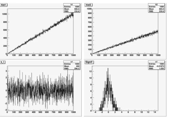
is a ratio of histograms volumes,σ2nˆi1,σ2nˆi2are variances of number of events in bin #i. An example is presented in Fig.2. HereK =2,σ2nˆi1 =nˆi1,σ2nˆi2 =nˆi2,iis changed from 1 up to 1000.
4.1.1 Consistency or distinguishability of histograms
Often a goal of histograms comparison is a testing of their consistency. Consistency here is the statement that both histograms are produced during data processing of independent sam-ples which are taken from the same flow of events (or from the same population of events).
Figure 2. Triangle distributions: (a) the observed values ˆni1in the first histogram (left,upper), (b) the
observed values ˆni2in the second histogram (right, upper), (c) observed significances ˆSibin-by-bin (left,
bottom), (d) the distribution of observed significances ˆSi(right, bottom).
4.1.2 “Distance” between histograms
We can calculate statistical moments for distribution of ˆSi (Fig.2(d)) and, in principle, we
have information about distinguishability of samples under testing. Here we consider two moments: the mean value of significances distribution ¯S and therms(root mean square) of this distribution, i.e. bidimensional test statisticsS RMS =( ¯S,rms) as a “distance” between histograms [1, 2]:
a) ifS RMS =(0,0), then histograms are identical;
b)ifS RMS ≈(0,1), then samples are taken from the same flow of events; c) if previous conditions are not valid, the flows of events have difference.
4.2 Comparison of dependences
We can applied this approach for comparison of pair of dependences. The another formula
ˆ
Si= nˆi1−nˆi2
σ2nˆi1+σ2nˆi2
, (9)
whereiis number of point in dependences for independent variable, ˆnimis value of dependent
variable in pointifor dependencem,m=1,2,σnˆ2i1,σ2nˆi2 are variances of dependent variable in point #i, is used in this case.
4.2.1 Hypotheses testing
The using of approach described above for comparison of data has many problems, which can be avoid with the help of the method of repeated dependence. If the goal of the comparison of dependences is the check of their consistency, then task is reduced to hypotheses testing: main hypothesis H0 (dependences are produced during data processing of samples taken from the same flow of events) against alternative hypothesisH1 (dependences are produced during data processing of samples taken from different flows of events). The determination of critical area allows to estimate Type I error (α) and Type II error (β) in decision about choice betweenH0 andH1. The Type I error is a probability of mistake if done choice isH1, but H0 is true. The Type II error is a probability of mistake if done choice isH0, butH1 is true.
DistributionH0 is a confidence density of expected value of test statistics (which is used for hypotheses testing) if hypothesis H0 is true, distribution H1 is a confidence density of expected value of test statistics if hypothesisH1 is true.
The selection of a significance level (α) allows to estimate the power of the test (1−β). Usually, the values of significance level are 10%, 5% or 1%.
If both hypotheses are equivalent, then other combinations of theαandβare used. For example, in task about distinguishability of the flows of events works a relative uncertainty
α+β
2−(α+β) forα+β≤1 [21]. Under the test of equal tails [21, 22] the mean error α+β
2 can be used.
4.2.2 Method of repeated dependence
The hypotheses testing require the knowledge of the distribution of test statistics. The dis-tribution of test statistics can be constructed by Monte Carlo. If errors of values in mea-sured points of at least one of dependence (for example, reference) are known, than one can construct the set of similar dependences (clones) according with errors, which imitates the population of dependences which produced due to data processing of the samples taken from the same flow of events. This set of dependences is used for construction of the distribu-tion of reference statistics for the case ofH0 hypothesis (due to comparison of the reference dependence and the produced clones of the reference dependence). This procedure can be named as ”method of repeated dependence" in analogy with ”method of repeated sample" or “resampling” in bootstrap technique [23].
Further the set of dependences of such type is constructed for test dependence (second dependence under comparing). New set is used for construction of the distribution of test statistics for the case ofH1 hypothesis. This is comparison of the reference dependence with the produced clones of test dependence (i.e. with clones of second dependence).
The comparison of the distribution of reference statistics for the case of H0 hypothesis (imitation population ofS RMS, which produced by the comparing of reference dependence and its clones) and the distribution of test statistics for the case ofH1 hypothesis (imitation population ofS RMS, which produced by the comparing of reference dependence and clones of test dependence) allows to estimate the uncertainty in hypotheses testing. Note, there are another combinations for comparison depending on task (reference clones with test clones and so on). The procedure is used in paper [3]. The application of this procedure in the case of histogram comparison can be found in paper [2].
5 Conclusion: advantages of this approach
• We can compare multidimensional dependences likewise as unidimensional dependences. • We can compare two sets of several dependences simultanously likewise as we compare a
pair of dependences.
• We can use any unidimensional test statistics (Kolmogorov-Smirnov, Anderson-Darling, ...) as additional dimension in proposed multidimensional test statistics.
The authors are grateful to V.A. Kachanov, V.A. Matveev and N.E. Tyurin for the interest and support. We thanks Yu.P. Gouz, S.V. Erin, A.M. Gordeenko, Yu.V. Kharlov, I.B. Smirnov, V.A. Taperechkina and M.N. Ukhanov for fruitful discussions.
References
[1] S. Bityukov, N. Krasnikov, A. Nikitenko, V. Smirnova, arXiv:1302.2651 (2013)
[2] S. Bityukov, N. Krasnikov, A. Nikitenko, V. Smirnova, Eur.Phys. J. Plus128:143(2013) [3] S.I. Bityukov, N.V. Krasnikov, A.N. Nikitenko, A.V. Maksimushkina, V.V. Smirnova,
Izvestiya vuzov. Yadernaya energetika3, 43-51 (2014)
[4] B. Krupanek, R. Bogacz, Przeglad Elektrotechniczny1132-34 (2014)
[5] Q. Chu, J. Liu, K. Bali, K. R. Thorp, R. Smith and G. (Sam) Wang, HortTechnology26 no. 1 (2016) 12-19
[6] E. Contreras-Hernandez, D. Chavez, E. Hernandez et al., J. Physiol.596(9), 1747-1776 (2018)
[7] S. Bityukov, N. Krasnikov, S. Nadarajah, V. Smirnova, Applied Mathematics5, 963-968 (2014)
[8] S. Bityukov, N. Krasnikov, S. Nadarajah, V. Smirnova, AIP Conference Proceedings 1305, 346-353 (2011)
[9] J.M. Bernardo and A.F.M. Smith,Bayesian Theory(John Wiley and Sons, Chichester, 1994)
[10] S. Bityukov, V. Smirnova, V. Tapereckina, arXiv:math/0411462 (2004)
[11] M. Blackwell, J. Honaker, and G. King, Sociological Methods & Research46, 342-369 (2017)
[12] V.E. Jennings, C.W. Lloid-Smith, Mathematical Scientist40, 103-117 (2015) [13] S. Bityukov, V. Medvedev, V. Smirnova, Yu. Zernii, arXiv:physics/0403069 (2004) [14] Min-ge Xie and Kesar Singh, International Statistical Review81, 3 (2013) [15] S. Nadarajah, S. Bityukov, N. Krasnikov, Statistical Methodology22, 23 (2015) [16] Y. Zhu, High Ener. Phys. Nucl. Phys. 30, 331-334 (2006); arXiv:physics/0507145
(2005)
[17] S.I. Bityukov, N.V. Krasnikov, Nucl.Instr.&Meth.A452518-524 (2000) [18] S. Bityukov, N. Krasnikov, A. Nikitenko, arXiv:physics/0612178 (2006)
[19] S.I. Bityukov, N.V. Krasnikov, A.N. Nikitenko, V.V. Smirnova, Proceedings of Science ACAT2008, 118 (2008)
[20] M. Fisz, Colloquium Mathematicum3, 199-202 (1955)