171 | P a g e
ANALYSIS AND SELECTION OF A QUANTITATIVE
FORECASTING MODEL FOR AN ENTERPRISE IN
THE ELECTRONIC SECTOR
Ing. Marissa González Luna
1, Dr. Manuel Alonso Rodríguez Morachis
2 1Student of the
Masters in Administrative Engineering in the Division of Graduate Studies
and Research of the Technological Institute of Ciudad Juárez.
2
Research Professor of the Division of Postgraduate Studies
and Research of the Technological Institute of Ciudad Juárez, Mexico.
ABSTRACT
In today's business environment, a company's success depends largely on good management of its supply chain.
Problems are often encountered at the beginning of the supply chain, which is the procurement of materials, due
to poor planning of customer demand and misalignment of sales forecasts into the future. In this article, the
historical data of an electronic company is analyzed, to select the best quantitative forecast model comparing the
methods of Simple and Double Exponential Smoothing and Hold-Winters Smoothing.
Keywords
:
Double Exponential Smoothing, Forecasting Methods, Hold-Winters, Inventory
Control, Simple Exponential Smoothing, Supply Chain.
I. INTRODUCTION
The manufacturing activity is encompassed in the supply chain activities, ranging from procurement of materials
to customer service and delivery. Based on this, it can be said that everything starts with a good prediction of
what is going to happen in the future, knowing that, the company assures its survival in the market by always
being ahead in the prediction of the future demands of the customers.
Many of the forecasting techniques in use today were developed in the 19th century. Before the advent of more
sophisticated forecasting techniques and computer power, the administrator's judgment was the only possible
forecasting tool [1].
García et al. (2009) analyzes that according to Hanke and Reitsch (1996) the forecasts can be classified into two
main criteria: the first criterion is time, that is, there are short and long term forecasts. The latter helps to
establish the general course of the organization over a long period of time, while the former is used to design
strategies that will have immediate use and will be implemented by middle levels in the organization. The
second type of criterion classifies forecasts in qualitative and quantitative; the first is applied when a person's
judgment is issued, while the quantitative ones refer to mechanical processes that result in mathematical data
[2].
In the company investigated, the best quantitative forecast model was analyzed with the objective of
172 | P a g e
goods and that the production plan is also handled by different people, which in turn can manage the samematerials. In addition, material losses due to waste, quality defect or loss, as well as sudden client orders were
taken into consideration.
Rodriguez-Coy and Rodríguez-Morachis (2010) assert that the forecast of the demand has always been
an important issue in the administration and control of operations; activities such as decision making, inventory
management, new product development, production, and supply chain planning all require a good forecast
prediction [3].
According to Chapman (2006), a basic forecasting concept would be: The formulation of forecasts (or
projection) is a technique that uses past experiences in order to predict future expectations. Some characteristics
of the demand forecasts are [4]:
Demand forecasting typically originates in marketing [5].
The forecastsupports the decisions that are based on it [6].
All the forecasts will be wrong, some will exceed the demand and others will be below it, the secret for the
forecast to be successful is to choose the technique that offers the least amount of error [7].
Quantitative methods are more accurate and convenient to use if historical data is available [8].
II. MATERIALS AND METHODS.
In this section, the historical data of an electronic company is analyzed, to select the best quantitative forecast
model comparing the methods of Simple and Double Exponential Smoothing and Hold-Winters Smoothing.
2.1 Simple Exponential Smoothing Methodology.
This is one of the techniques most used in forecasting. In the exponential smoothing method, only three pieces
of data are needed to forecast the future: the most recent forecast, the actual demand that occurred during the
forecast period and an alpha uniformity constant (α). This smoothing constant determines the level of uniformity
and rate of reaction to the differences between forecasts and real occurrences [9]:
The equation for a single forecast is:
(1)
Where:
Ft= Prognosis smoothed exponentially for period t.
Ft-1= The forecast smoothed exponentially for the previous period.
At-1= The real demand for the previous period.
α = The response rate or the smoothing constant.
This equation establishes that the new forecast is equal to the previous forecast plus a portion of the error.
For the choice of the appropriate value of alpha, exponential smoothing requires giving the smoothing constant
173 | P a g e
effects of the short term or random changes. If real demand increases or decreases rapidly, a high alpha isdesired in order to provide a better track to the demand change [9].
2.2 Double Exponential Smoothing Methodology.
If a trend model were to be predicted using simple exponential smoothing, the forecast would have a delayed
growth reaction. The forecast would then tend to underestimate the real demand. To correct this, one can
estimate the slope and multiply the estimate by the number of future periods to be forecast. Dual exponential
smoothing incorporates the influence of trend and seasonality when specific values for these components can be
identified. The calculation of double exponential smoothing is similar to that of the basic smoothing model,
except that there are three components and three smoothing constants to represent the components: basic, trend,
and seasonal[10].
The system of equations is as follows [1]:
The series smoothed exponentially or estimated current level.
(2)
The estimate of the trend.
(3)
The forecast for the pperiods of the future.
(4)
Where:
Lt= New smoothed value (current level estimate).
α = smoothing constant for the level (0 <α <1)
Yt= New observation or actual value of the series in period t.
β = Smoothing constant for the trend estimate (0 <α <1).
Tt = Trend estimate.
P = Periods to be forecast in the future.
Forecast for period p in the future
.
2.3 Hold-Winters Smoothing Methodology.
The Winters method is a useful procedure when there is tendency and seasonality, and these two components
are additive or multiplicative. The Winters Method calculates dynamic estimates for three components: level,
174 | P a g e
The initial values for the level and trend components are obtained from a linear regression over time. The initialvalues for the seasonal component are obtained from a regression of indicator variables using data without trend
[11].
There are two models of the Winters formulas, the multiplicative and the additive. The multiplicative model is
used when the magnitude of the seasonal pattern increases as the data values increase and/or decreases as the
data values decrease. The additive model is used when the magnitude of the station pattern does not change
when the series goes up or down. If the pattern in the data is not very obvious and there is trouble choosing
between additive and multiplicative procedures, both procedures can be used and the one with the smallest
accuracy measurements can be chosen. The following equations are the smoothing equations of the
Hold-Winters method [11]:
Smoothing equation for the additive model:
(5)
(6)
(7)
(8)
Smoothing equation for the multiplicative model:
(9)
(10)
(11)
(12)
Where:
Lt = Level at time t.
α = The weighting for the level.
Tt = Trend estimate at time t.
= Weighting for the trend.
St = The seasonal component at time t.
= The weighting for the seasonal component.
P = The seasonal period.
Yt = Value of the data at time t.
Forecast in a period ahead in time t.
2.4 Forecast Error.
According to Ballou (2004). The forecast error is defined as [12]:
(13)
Where:
175 | P a g e
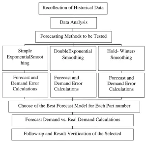
Follow-up and Result Verification of the SelectedModels.
Forecast Demand vs. Real Demand Calculations Choose of the Best Forecast Model for Each Part number Forecast and Demand Error Calculations Forecast and Demand Error Calculations Forecast and Demand Error Calculations Simple ExponentialSmoot hing DoubleExponential Smoothing Hold- Winters Smoothing Forecasting Methods to be Tested
Data Analysis Recollection of Historical Data DR= Actual demand.
Dp= Forecast demand.
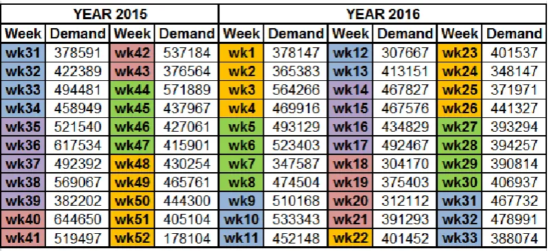
For this investigation, the historical data of 55 periods were collected. A period includes the use plus the waste
of material, each period represent a week. Samples were taken from two part numbers, 300-05798 key product
for the customer and high value part; N10-2222LF high volume and common use in 53% of the products
manufactured by the company.
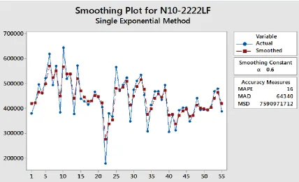
The software used for the research is Minitab 17 Statistical Software®, this application provided several options
of forecast models, with which it was possible to define the trend of the data and to provide an adequate forecast
for data collected.
Figure 1 shows in general the steps to follow in the methodology for this research, after the
identification of the problem what follows is the collection of the data and the analysis of the same, analysis
shows that both numbers obey horizontal patterns and / or seasonal, it is for this reason that the following
methods that estimate these types of patterns will be tested: Simple Exponential Smoothing, Double Exponential
Smoothing, and Hold- Winters Smoothing.
176 | P a g e
The following is the data collected by 55 periods and are shown in Tables 1 and 2:Table 1.Calculated Quantity of Use Plus the Delay in Sales (300-05798).
Table 2. Calculated Quantity of Use Plus the Delay in Sales (N10-2222LF).
After observing the patterns of the data, a normality test was applied, which indicates that the data has a normal
trend and parametric tests of averages comparison and tests of variances can be used, in order to demonstrate the
hypothesis that the real data is statistically equivalent to those predicted for each of the selected models.
To present results and select the best forecast model, after having obtained the calculations for the three selected
models, comparing the forecast demand vs. the real demand, in addition to reviewing the forecast error where
the error is smaller and the forecast is closer to the real demand would be the most appropriate method.
177 | P a g e
Figure 2. Double Exponential Smoothing With Values of 0.9 and of 0.05 (300-05897).Figure 3. Simple Exponential Smoothing with Values of 0.6 (N10-2222LF).
III. RESULTS.
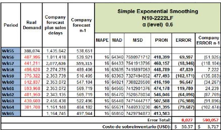
After nine weeks of follow-up to the selected models for each part number, the conclusion is that the models
continue to give a good fit to the actual data in Tables 3 and 4.The tables show the results week to week of
178 | P a g e
purchasing department, with the aim of comparing the proposal of this research work against what is currentlyimplemented by the company.
Table 3.Follow-up to Number 300-05798.
179 | P a g e
In reviewing tables 3 and 4, a better follow-up of the forecast models proposed in this research is seenthan the forecasts currently being handled by the company. If the change in the wayof forecasting data is
implemented, only in these two part numbers taken from the sample it will generate a reduction in the cost of
maintaining inventory of $408,658.43 American dollars in just 9 weeks.
IV. DISCUSSION.
At the beginning of this investigation it was found that the company did not have a method to calculate demand
forecasts in a reliable way, since the same department of marketing is aware that the demand they present to the
purchasing department has an accuracy of the 46%, leading the company to have over inventory of materials
that does not require up to fourteen million dollars, with a sales delay of sixteen million dollars.
It is thus decided to analyze the historical data collected for 55 weeks and to calculate a better forecast
by means of quantitative methods, and after testing several methods, it is concluded that for the part number
300-05791 reliable demands can be obtained using the Double Exponential Smoothing method and for the
N10-2222LF good results are obtained using the Simple Exponential Smoothing method.
The methodology described in the research is not exclusive to only those two part numbers, since it has
mathematical validity, it is recommended to extend this analysis to the rest of the products that represent a
problem in the company, since these numbers model the greater part of the behaviors of the finished products
that the company produces. Greater benefits can be obtained in the planning of its raw materials as well as
reduction of costs by maintenance of inventory.
In addition, considering that the models investigated are of universal validity, their application in other
products of different branches in the manufacturing industry is recommended, since as has been seen in other
investigations carried out in other companies of the manufacturing sector of the region, quantitative forecasting
methods have solved the problem of calculating demand forecasts in each of the case studies.
REFERENCES
[1] Hanke J. y Wichern D (2010). Pronósticos en los negocios. 9na. Ed. Pearson Educación. Naucalpan de
Juárez, Estado de México, México.
[2] García S. A., Vázquez C. D., Reyes O. H., Sáenz S. A., Limón L. A. (2009). Investigación en el ámbito
empresarial “Pronósticos, supervisión e indicadores financieros” (Estudios de casos) Edición electrónica
Texto completo en www.eumed.net/
[3] Rodríguez-Coy. M. y Rodríguez-Morachis. M. (2010). Aplicación de Métodos de Pronósticos en Productos
con Demandas Inciertas. 3er. Congreso Internacional de Investigación CIPITECH, (3), 8, 618-624.
[4] Chapman S. (2006). Planificación y control de la producción. México: Pearson. Naucalpan de Juárez,
Estado de México, México.
[5] Krajewski L., Ritzman L. y Manhotra M. (2008). Administración de Operaciones: Procesos y Cadena de
Valor. 8va Ed. Pearson Educación Naucalpan de Juárez, Estado de México, México.
[6] Chopra, S. y Meindl, P. (2008). Administración de la Cadena de Suministro. Estrategia, Planeación y
180 | P a g e
[7] Coyle J., Langley J., Novack R. y Gibson Brian (2013). Administración de la cadena de suministros. 9na.Ed. Cengage Learning. Pennsylvania, EE.UU.
[8] Nahmias S. (2007). Análisis de la producción y las operaciones. 6ta. Ed. McGraw-Hill México, D.F.
México.
[9] Chase R., Jacobs R. y Aquilano N. (2009) Administración de operaciones: Producción y cadena de
suministros. 12ma Ed. McGraw-Hill. México D.F. México.
[10] Bowersox D, Closs D y Cooper M. (2007).Administración y logística en la cadena de suministros. 2da
Ed.McGraw-Hill. México D.F. México.
[11] Minitab Inc., “Métodos para analizar series de tiempo”. (Documento Web Copyright © 2016).
http://support.minitab.com/es-mx/minitab/17/topic-library/modeling-statistics/time-series/basics/methods-for-analyzing-time-series/ September 25th 2016.
[12] Ballou R. (2004). Logística: Administración de la cadena de suministro. 5ta Ed.Pearson Educación.