DOI: 10.12928/TELKOMNIKA.v14i1.2812 245
Hybridizing PSO with SA for Optimizing SVR Applied to
Software Effort Estimation
Dinda Novitasari, Imam Cholissodin, Wayan Firdaus Mahmudy Dept. of Informatics/ Computer Science, Brawijaya University, Malang 65145 e-mail: [email protected], [email protected], [email protected]
Abstract
This study investigates Particle Swarm Optimization (PSO) hybridization with Simulated Annealing (SA) to optimize Support Vector Machine (SVR). The optimized SVR is used for software effort estimation. The optimization of SVR consists of two sub-problems that must be solved simultaneously; the first is input feature selection that influences method accuracy and computing time. The next sub-problem is finding optimal SVR parameter that each parameter gives significant impact to method performance. To deal with a huge number of candidate solutions of the problems, a powerful approach is required. The proposed approach takes advantages of good solution quality from PSO and SA. We introduce SA based acceptance rule to accept new position in PSO. The SA parameter selection is introduced to improve the quality as stochastic algorithm is sensitive to its parameter. The comparative works have been between PSO in quality of solution and computing time. According to the results, the proposed model outperforms PSO SVR in quality of solution.
Keywords: Particle swarm optimization, simulated annealing, support vector regression, feature selection, parameter optimization
Copyright © 2016 Universitas Ahmad Dahlan. All rights reserved.
1. Introduction
The most important part of software project is software effort estimation. It determines how many resources that project needed and must be done accurately. If we have big error rate in estimation, it will lead into big loss such as unpredictable delay time and unexpected budget. To prevent many losses in the future, some approaches are developed to estimate software effort. One of them is machine learning. Support vector machine is machine learning algorithm introduced by Vapnik to solve classification problem. Due to solve real world problems, SVM was developed to solve regression and time series prediction called SVM based regression (SVR). In order to solve nonlinear regression problem, SVR mapped data to high dimensional feature space using kernel function. This kernel must satisfy Mercer condition [1] and one of kernels is radial basis function (RBF).
In machine learning, feature selection introduced as a process of selecting a subset feature for use in model construction. This process is needed for SVR since it can simplify computing process and reducing computing time, especially when computing in high dimensional space. Besides that, proper parameter settings can influence SVR accuracy. SVR-RBF has parameters influenced its performance i.e. error penalty, insensitive loss, and radial basis [2]. Those mentioned above are crucial in SVR-RBF because feature selection influences SVR parameter and vice versa [3]. In the past research, Oliviera investigated the use of SVR in order to do software effort estimation [4]. It gives promising result but cannot guarantee give good result since using predefined number of features and parameter means cannot discover other options that can lead into higher accuracy rate. Numerous candidate of solution can be generated in order to have great number of subset feature combination and vary range of parameter, if we use enumeration. However, it does not utilize a fitness function, and is thus unguided, often failing to find good solution. Due to the complexity of the problem, a powerful approach is required to get a good solution.
Some stochastic optimization methods become alternative to select subset feature and optimize parameter. It generates candidate solutions, involves objective function to evaluate the quality of solution so solution searching could be lead into a good solution. Braga et al proposed genetic algorithm (GA) to optimize SVR in software effort estimation [5]. Our previous research
proposed particle swarm optimization (PSO) to optimize SVR in the same problem domain [6]. Basically, PSO is inspired by flocking bird motion employed parallel search techniques, exploitation and exploration. However, PSO has disadvantage, trapped in local minimum because particles move in high velocity and gain premature convergence [7]. On the other hand, simulated annealing inspired by process of annealing in metallurgy, is good in finding local optimum [8]. Therefore, this study investigates hybridization PSO with SA in order to enhance searching capacity. This proposed model is used to optimize SVR parameter and select subset feature applied to software effort estimation.
Several researches investigated SVR optimization have been done and gained promising result. Braga et.al [5] investigated GA application to select subset feature and SVR parameter applied to software effort estimation. They used binary coded chromosome as solution representation for subset feature and SVR parameter. Their research reported success to improve SVR performance. Our previous research [6] investigated PSO application to select subset feature and SVR parameter applied to software effort estimation. We used continuous value type to optimize SVR parameter and discrete value type to select subset feature. Another effort has been done by Adhani [9], who optimized SVR with GAPSO. They are reported success to build SVR model for predicting rainfall in dry season. However, other researches have been done to investigate on how to improve PSO performance. Xue [10] introduced QoS-based hybrid particle swarm optimization (GHPSO) to schedule workflow in cloud computing. It gained better performance than PSO. A research conducted by Shieh et.al [11] in modification PSO with SA. Their research proposed SAPSO to enhance searching capacity algorithm. They reported proposed model could have higher efficiency, better quality and faster convergence than PSO. Therefore, based on past researches, this study proposed SAPSO SVR applied to software effort estimation. By using SAPSO, can be generated more optimize SVR parameter, better selected feature, and low cost value.
2. Support Vector Regression
Given training data {xi,yi}, i = 1,...,l; xi∈ Rd; yi∈Rd where xi, yi is input (vector) and
output (scalar value as target). Other forms of alternative for bias to calculation f(x) is can be build solution like bias as follows [1]:
l i i i i k k l i i i i k k k T k x x k y x x y x w y b 1 * 1 * , , (1)xi is support vector where |αi- αi*| isn’t zero. Equation f(x) can be written as follows:
x
x x
b f l i i i i
1 * (2)Lambda (λ) is scalar constant, with it’san augmented factor defined as follows [12]:
. ) ) , ( )( ( ) ( 1 2 *
l i i i i x x K x f
(3)2.1. Sequential Algorithm for SVR
Vijayakumar has made tactical steps through the process of iteration to obtain the solution of optimization problems of any nature by way of a trade-off on the values of the weights xi, or called αi to make the results of the regression becomes closer to actual value. The
step by step as follows [12]:
1. Initializei 0,*i 0. Compute 2 ) , ( ] [RijK xi xj (4) for i,j = 1,…,n
n j i i ij i i y R E 1(
*
) (5) }. ], ), ( min{max[ * * * i i i i E C (6) }. ], ), ( min{max[ i i i i E C (7) . * * * i i i
(8).
i i i
(9)3. Repeat step 2 until meet stop condition. Where learning rate γ is computed from:
diagonal of kernel matrice
max
constant rate
learning
(10) 3. Particle Swarm Optimization
Particle swarm optimization was introduced by Kennedy and Ebenhart [13], as a nature inspired algorithm. Particles are defined as solution for problem. Developing by Shi and Ebenhart [14], PSO is added by inertia weight to improves performance. Each particle has position and velocity, and updates that in every iterating. The velocity is updated by:
vij(t+1)=wvij(t)+c1r1j(t)[yij(t)-xij(t)]+c2r2j(t)[ŷ(t)-xij(t)] (15)
And its position updated by:
xi(t+1)=xi(t)+vi(t+1) (16)
Where vij(t) is velocity of particle i in dimension j=1,...n at time t, xij(t) is position of
particle i in dimension j at time t, c1 and c2 are acceleration constants used to scale contribution
of the cognitive and social components, r1j and r2j are random values in the range [0,1]. W is
inertia weight obtained by:
max max max min max iter iter iter (17)Where wmax and wmin are maximal and minimum inertia weight, itermax is maximum
number of iterations, iter is current iteration number. Yi is personal best position of particle i
obtained by:
t i y f t i x f t i x t i y f t i x f t i y t i y 1 if 1 1 if 1 (18)And ŷ represents global best position of particle i obtained by:
Ŷ(t)∈ {y0(t),…,yns(t)}|f(ŷ(t))=min {f(y0(t)),…, f(yns(t))} (19) 3.1. Binary PSO
Some optimization problems are set in a space featuring discrete. Kennedy and Ebenhart [15] proposed binary PSO in which each element of particle’s position vector can take on the binary value 0 or 1. New velocity of particle is normalized by sigmoid function:
ij
v t ij ij e t v sig t v 1 1 (20) Where vij(t) is obtained from Equation (15). Using Equation (16), the position update changes to:
otherwise 0 1 if 1 1 r3 t sigv t t xij j ij (21) Where r3j(t) ~ U(0,1).4. Hybridizing PSO with SA
A searching algorithm has two important components, exploration and exploitation. Exploration means algorithm search in different region of searching space to find global optimum. Exploitation means algorithm localize promising area to find best solution in that area. A good searching algorithm must able to balance its exploration and exploitation, able to search entire space and jump out of local optimum solution. By that means, it must able to improve probability and ability of finding global optimum solution.
Initial random position PSO can lead into premature convergence, entire particle move toward local optimum solution and cause weakening exploration because particle can’t jump out of area. It is characteristic and weakness of PSO. Meanwhile, SA with low variation of temperature parameter and searching solution reach equilibrium condition, able to guarantee to find global optimum. It is enhanced by metropolis process, ability to jump out from local optimum. However, it costs high computing time.
Based on PSO and SA characteristic above, this study hybridizes PSO with SA, combines PSO parallel process and movement mechanism and SA searching procedure. By combining that, this proposed model able to find good solution in local and global optimum with low computing time.
4.1. Simulated Annealing Algorithm
Simulated annealing is an optimization process based on the annealing process; the cooling process of a liquid or solid and the analysis of the behavior of substances as they cool. This algorithm is introduced by Kirkpatrick [16] and inspired by Metropolis work about energy distribution [17]. In SA algorithm, metropolis process does searching solution. During the process, disturbance mechanism (metropolis acceptance rule) determines quality of solution by searching around existing solution and comparing neighbor solution and current solution. This procedure affects SA ability to jump out from local optimum solution. If neighbor solution is better than current solution then neighboring solution is accepted as the new current solution. If neighbor solution is worse than current solution then SA will use a probability to determine whether accept this neighboring solution as new current solution or not, or regenerate for a new neighboring solution. The probability mechanism for metropolis acceptance rule is defined as follows:
otherwise if 1 T c x f x f i j b i j e x f x f P (22)Where P is probability, f(xj) is neighbor solution, f(xi) is current solution, cb>0 is
Boltzmann constant and T is temperature of the system. T is derived from:
Tk+1=α x T0 (23)
Where α is cooling rate, Tk+1 is temperature at time k, and T0 is initial temperature.
While SA is quite simple, it has been successfully implemented to solve various combinatorial problem [18].
5. SAPSO SVR Model 5.1. Particle Representation
In this study, SVR RBF is defined by the parameter C – complexity parameter, ε- the extent to which deviations are tolerated, λ - augmenting factor, σ – width of RBF kernel, cLR – learning rate constant. The particle is comprised of six parts: C, ε, λ, σ, cLR (continuous-valued) and features mask (discrete-valued). Table 1 shows the representation of particle i with dimension nf+5 where nf is the number of features. The feature mask is Boolean that “1”
indicates the feature is selected and “0” indicates feature is not selected.
Table 1. Particle i is composed of six parts: c, ε, λ, ε, cLR and feature mask
Continuous-valued Discrete-valued
C ε λ σ cLR Feature mask
Xi,1 Xi,2 Xi,3 Xi,4 Xi,5 Xi,6, Xi,7 ,...,Xi,nf
5.2. Objective Function
Objective function is used to measure how optimal the generated solution. There are two types of objective function: fitness and cost. The higher fitness value means better solution. The lower cost value means better solution. In this study, cost typed is used as objective function because the purpose of this algorithm is to minimize error. Accuracy of prediction and number of selected features are criteria used to design cost function. Thus, the particle with high accuracy of prediction and small number of features produces a low prediction error. The prediction error has two predefined weights: WA for accuracy of prediction (95%) and WF for the
selected feature (5%) [19].
n i i i i A F A n MAPE 1 1 (24)
F n j j F A n f w MAPE w error F 1 (25)Where n is number of data, Ai is actual value and Fi is prediction value for data, fj is
value of feature mask where “1” represents that feature j is selected and “0” represents that feature j is not selected and nf is total number of features.
5.3. SAPSO SVR Algorithms
The SAPSO SVR algorithm is started by initialization of particle. Then, calculate cost and determine personal best position (pBest) and global best position (gBest). After that, update velocity and position. Usually, PSO automatically accept new position, however SAPSO SVR introduces SA metropolis acceptance rule in this step. This rule determines whether to accept new position or regenerate another candidate position based on cost function difference between new and old positions. This enables PSO to jump out from local optimum, improve quality of solution, and increase rate of convergence. Simulated annealing explores solution towards direction of pBest and gBest. The acceptance rule accepts or rejects new solution based on current temperature parameter and cost value difference. If candidate solution unable pass criteria then a new position generated using PSO and repeated until metropolis acceptance rule accept new position or upper bound of disturbance is reached. By this way, the model explores solution, improve exploration and spend low computing time since using PSO parallel processing.
Based on Figure 1, the whole procedure of SAPSO SVR is described as follows: 1. Normalizing data using
min max min x x x x xn (26)
Where x is the original data from dataset, xmin and xmax is the minimum and maximum value of
original data, and xn is normalized value.
2. Dividing data into k to determine training and testing data. 3. Initializing a population of particle randomly 0
1
s , v100i=1,2,…n, iter=0. 4. Calculating cost of 0
1
s by averaging error over k SVR training. 5. Updating pBest and gBest of each particle.
6. Updating inertia weight.
7. Repeat these steps until meet stopping condition a) Updating velocity 1
1
iter
v and position of each particle. b) Calculating cost of 1
1
iter
s by averaging error over k SVR training. c) Evaluate ∆cost=
iter
iters
s 1
1 1 cost
cost and generate random number R [0,1]. If
∆cost≤0, then accept new position with probability ONE. Otherwise, 1 1
iter
s
is accepted based on following criterion: tempt e cos y probabilit
≥R. Proceed to next step if all new positions are accepted or repeat step 7.1 until 7.3 for those particles failed to be accepted. Too many failures (i.e. 100 in our study) for same particle will force the last position will be accepted.
d) Updating pBest and gBest of each particle.
e) Updating inertia weight and temperature, set iter=iter+1.
8. If stopping criteria is satisfied, and then end iteration. If not, repeat step 7. In this study, stopping criteria is a given number of iterations.
9. Output the best solution gBest and its cost value.
6. Application SAPSO SVR in Software Effort Estimation 6.1. Simulation Settings
This study simulates 2 algorithms: PSO SVR and SAPSO SVR programmed using C#. For SAPSO SVR simulation, we use the same parameter and dataset that is obtained from [6] that conducted PSO SVR simulation. For software effort estimation, the inputs of SVR are Desharnais dataset [20]. The Desharnais dataset consists of 81 software projects described by 11 variables, 9 independent variables and 2 dependent variables. For the simulation, we decide to use 77 projects due to incomplete provided features and 7 independent variables (TeamExp, ManagerExp, Transactions, Entities, PointsAdjust, Envergure, and PointsNonAdjust) and 1 dependent variable (Effort). The PSO parameters were set as in Table 2.. Firstly, we run test to determine best parameter for SA (T0 and α) then simulations is performed and compared to
other algorithms.
Table 2. PSO parameter settings Number of fold
Population of particles Number of iterations Inertia weight(wmax, wmin)
Acceleration coefficient(c1, c2)
Parameter searching space 10 20 40 (0,9, 0,4) (2, 2) C (0,1-1500), ε (0,001-0,009), σ (0,1-4), λ(0,01-3), cLR (0,01-1,75) 6.2. Best Parameter
In stochastic algorithms, parameters have effect to quality of generated solution. In SA, initial temperature and cooling rate influence its performance. By observing parameters, we choose best parameter has lowest cost in each simulation.
Table 3 showed simulation to choose best initial temperature (T0). This simulation
conducted by increasing temperature by 10% from 50 up to 90 in each simulation and use cooling rate at 0,5. If T0 is too low then algorithm has possibility to not explore, makes converge
at local optimum. If T0 is too high, then it can increase computing time. This table showed that T0 at 90 give lowest cost.
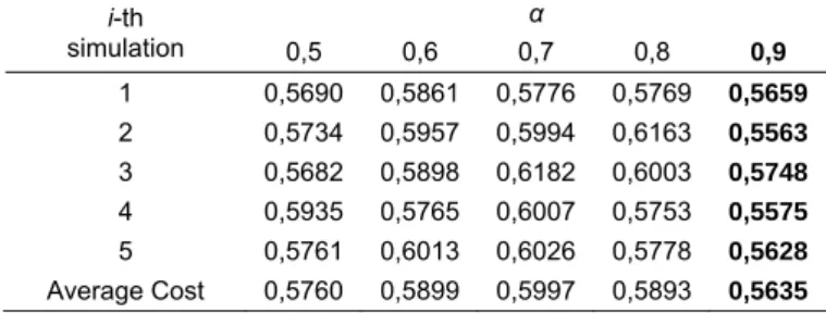
Table 4 showed simulation to choose best cooling rate (α). This simulation conducted by increasing temperature by 10% from 0,5 up to 0,9 in each simulation If α is too low then algorithm has possibility to fail into local optimum solution, repeats calculation, and increase computing time. If α is too high, then it increase computing time. This table showed that αat 0,9 give lowest cost.
Table 3. Parameter setting for initial temperature
i-th simulation T0 50 60 70 80 90 1 0,6084 0,8336 0,5801 0,6096 0,5690 2 0,5706 0,5760 0,7265 0,5975 0,5734 3 0,5992 0,5898 0,5886 0,5848 0,5682 4 0,5610 0,6177 0,6223 0,5875 0,5935 5 0,7475 0,7579 0,6161 0,5795 0,5761 Average Cost 0,6174 0,6750 0,6267 0,5918 0,5760
Table 4. Parameter setting for cooling rate
i-th simulation α 0,5 0,6 0,7 0,8 0,9 1 0,5690 0,5861 0,5776 0,5769 0,5659 2 0,5734 0,5957 0,5994 0,6163 0,5563 3 0,5682 0,5898 0,6182 0,6003 0,5748 4 0,5935 0,5765 0,6007 0,5753 0,5575 5 0,5761 0,6013 0,6026 0,5778 0,5628 Average Cost 0,5760 0,5899 0,5997 0,5893 0,5635
6.3. Comparison Works
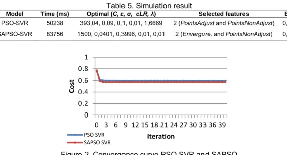
By using best parameter, we compare SAPSO SVR and PSO SVR performance. Figure 2 showed comparison of convergence between PSO SVR and SAPSO. It showed that SAPSO have faster convergence than PSO SVR. In Table 5, we can see that SAPSO has higher computing time faster than PSO SVR but on the other hand, SAPSO also can have faster convergence and lower cost than PSO SVR. The error difference of error is big, but the high computing time can be compromised. The computing time is high because the model must repeat searching candidate position if they fail meet the acceptance rule criteria and this is different with PSO automatically accept candidate position.
Table 5. Simulation result
Model Time (ms) Optimal (C, ε, σ, cLR, λ) Selected features Error
PSO-SVR 50238 393,04, 0,09, 0,1, 0,01, 1,6669 2 (PointsAdjust and PointsNonAdjust) 0,5981 SAPSO-SVR 83756 1500, 0,0401, 0,3996, 0,01, 0,01 2 (Envergure, and PointsNonAdjust) 0,5575
Figure 2. Convergence curve PSO SVR and SAPSO 7. Conclusion
This study investigated the use of SAPSO for optimal feature subset selection and SVR parameters optimization in the problem of software effort estimation. In our simulations, we used Desharnais dataset. We compared our results to PSO-SVR. From the experiment results, using SA can improve performance of PSO. The proposed model can combine the advantage of both algorithms and gain lower cost than PSO.
References
[1] Smola AJ, Scholkopf B. A Tutorial on Support Vector Regression. Statistics and Computing. 2004; 14(3): 199-222.
[2] Wang W, Xu Z, Lu W, Zhang X. Determination of The Spread Parameter in the Gaussian Kernel For Classification and Regression. Neurocomputing. 2003; 55: 643–663.
[3] Frohlich H, Chapelle O, Scholkopf B. Feature Selection for Support Vector Machines by Means of Genetic Algorithm. In Proceedings 15th IEEE International Conference on Tools with Artificial Intelligence. 2003: 142-148.
[4] Oliveira ALI. Estimation of software project effort with support vector regression. Neurocomputing. 2006; 69(13-15): 1749–53.
[5] Braga PL, Oliveira ALI, Meira SRL. A GA-based Feature Selection and Parameters Optimization for Support Vector Regression Applied to Software Effort Estimation. In Proceedings of the 2008 ACM Symposium on Applied Computing. Fortaleza, Ceará, Brazil, ACM. 2008: 1788–1792.
[6] Novitasari D, Cholissodin I, Mahmudy WF. Optimizing support vector regression using particle swarm optimization for software effort estimation. Submitted to: IAENG International Journal of Computer Science. 2015
[7] Shi Y, Eberhart RC. Empirical study of particle swarm optimization. In Proceedings of the 1999 Congress on Evolutionary Computation-CEC99. 1999: 1945–1950.
[8] Locatelli M. Convergence properties of simulated annealing for continuous global optimization. Journal of Applied Probability. 1996; 33(4): 1127–1140.
[9] Adhani G, Buono A, Faqih A. Optimization of Support Vector Regression using Genetic Algorithm and
0 0.2 0.4 0.6 0.8 1 0 3 6 9 12 15 18 21 24 27 30 33 36 39 Cost Iteration PSO SVR SAPSO SVR
Particle Swarm Optimization for Rainfall Prediction in Dry Season. TELKOMNIKA Indonesian Journal of Electrical Engineering. 2014; 12(11): 7912–7919.
[10] Xue S, Wu W. Scheduling Workflow in Cloud Computing Based on Hybrid Particle Swarm Algorithm.
TELKOMNIKA Indonesian Journal of Electrical Engineering. 2012; 10(7): 1560–1566.
[11] Shieh H-L, Kuo C-C, Chiang C-M. Modified particle swarm optimization algorithm with simulated annealing behavior and its numerical verification. Applied Mathematics and Computation. 2011; 218(8): 4365–4383.
[12] Vijayakumar S, Wu S. Sequential Support Vector Classifiers and Regression. In Proceedings of International Conference on Soft Computing (SOCO ‘99). 1999: 610–619.
[13] Kennedy J, Eberhart R. Particle Swarm Optimization. In Proceedings of IEEE International Conference on Neural Networks. Piscataway, NJ. 1995: 1942–1948.
[14] Shi Y, Eberhart R. A Modified Particle Swarm Optimizer. In 1998 IEEE International Conference on Evolutionary Computation Proceedings IEEE World Congress on Computational Intelligence. 1998: 69–73.
[15] Kennedy J, Eberhart RC. A discrete binary version of the particle swarm algorithm. In Proceedings of the World Miulticonference on Systemics, Cybernetics and Informatics. Piscataway, NJ. 1997: 4104– 4109.
[16] Kirkpatrick S, Gelatt CD, Vecchi MP. Optimization by Simulated Annealing. Science. 1983; 220(4598): 671–680.
[17] Metropolis N, Rosenbluth AW, Rosenbluth MN, Teller AH, Teller E. Equation of State Calculations by Fast Computing Machines. Journal of Chemical Physics. 1953 ;1087(21).
[18] Mahmudy WF. Improved simulated annealing for optimization of vehicle routing problem with time windows (VRPTW). Kursor. 2014; 7(3): 109–116.
[19] Guo Y. An Integrated PSO for Parameter Determination and Feature Selection of SVR and Its Application in STLF. In Proceedings of the Eighth International Conference on Machine Learning and Cybernetics. Baoding. 2009: 12–15.
[20] Sayyad Shirabad J, Menzies TJ. The PROMISE Repository of Software Engineering Databases [Internet]. School of Information Technology and Engineering, University of Ottawa, Canada. 2005.