Equalization for MIMO Underwater Acoustic Communications
.
White Rose Research Online URL for this paper:
http://eprints.whiterose.ac.uk/126318/
Version: Accepted Version
Article:
Zhang, Youwen, Zakharov, Yuriy and Li, Jianghui (Accepted: 2018) Soft-Decision-Driven
Sparse Channel Estimation and Turbo Equalization for MIMO Underwater Acoustic
Communications. IEEE Access. ISSN 2169-3536 (In Press)
[email protected] https://eprints.whiterose.ac.uk/
Reuse
Unless indicated otherwise, fulltext items are protected by copyright with all rights reserved. The copyright exception in section 29 of the Copyright, Designs and Patents Act 1988 allows the making of a single copy solely for the purpose of non-commercial research or private study within the limits of fair dealing. The publisher or other rights-holder may allow further reproduction and re-use of this version - refer to the White Rose Research Online record for this item. Where records identify the publisher as the copyright holder, users can verify any specific terms of use on the publisher’s website.
Takedown
If you consider content in White Rose Research Online to be in breach of UK law, please notify us by
Soft-Decision-Driven Sparse Channel Estimation
and Turbo Equalization for MIMO Underwater
Acoustic Communications
Youwen Zhang, Yuriy Zakharov, Senior Member, IEEE, Jianghui Li, Member, IEEE
Abstract—Multi-input multi-output (MIMO) detection based on turbo principle has been shown to provide a great enhance-ment in the throughput and reliability of underwater acoustic (UWA) communication systems. Benefits of the iterative detection in MIMO systems, however, can be obtained only when a high quality channel estimation is ensured. In this paper, we develop a new soft-decision-driven sparse channel estimation and turbo equalization scheme in the triply selective MIMO UWA. First, the Homotopy recursive least square dichotomous coordinate descent (Homotopy RLS-DCD) adaptive algorithm, recently proposed for sparse single-input single-output (SISO) system identification, is extended to adaptively estimate rapid time-varying MIMO sparse channels. Next, the more reliable a posteriori soft-decision symbols, instead of the hard decision symbols or the a priori soft-decision symbols, at the equalizer output, are not only feedback to the Homotopy RLS-DCD based channel estimator but also to the minimum mean-square-error (MMSE) equalizer. As the turbo iterations progress, the accuracy of channel estimation and the quality of the MMSE equalizer are improved gradually, leading to the enhancement in the turbo equalization performance. This also allows the reduction in pilot overhead. The proposed receiver has been tested by using the data collected from the SHLake2013 experiment. The performance of the receiver is evaluated for various modulation schemes, channel estimators and MIMO sizes. Experimental results demonstrate that the proposed a posteriori soft-decision-driven sparse channel estimation based on the Homotopy RLS-DCD algorithm and turbo equalization offer considerable improvement in system performance over other turbo equalization schemes.
Index Terms—A posteriori soft-decision, a priori soft-decision,
channel estimation, DCD iterations, Homotopy iterations,
multiple-input multiple-output (MIMO), recursive least-squares (RLS), sparse channel, turbo equalization, underwater acoustic communication.
I. INTRODUCTION
In recent years, the terrestrial wireless communication has made great achievements, However, wireless communication underwater, more specifically, the underwater acoustic com-munication, is still facing significant challenges incurred by the harsh underwater acoustic propagation environment [1]– [8]. Unlike the terrestrial radio channel, the UWA channel is featured by frequency-dependent limited bandwidth, long
Youwen Zhang is with the Acoustic Science and Technology Labora-tory and the College of Underwater Acoustic Engineering, Harbin Engi-neering University, Harbin, Heilongjiang, 150001, China. Email: [email protected].
Yuriy Zakharov is with the Department of Electronic Engineering, Univer-sity of York, York, YO10 5DD, UK. Email: [email protected].
Jianghui Li is with the Institute of Sound and Vibration Research, University of Southampton, U.K., e-mail: [email protected].
delay spread and rapid time variation due to severe Doppler effects (caused by the low speed of sound in water), leading to relatively low data rates in a range between a few bits/s (bps) to several tens of kbits/s (kbps) and often unsatisfied performance. The UWA channel has been regarded as one of the most difficult channels for communications [8], [10].
Generally, two families of modulation techniques, single-carrier modulation and multisingle-carrier modulation, are widely investigated in UWA communications [10], [12]–[14]. These two types of modulation have their own advantages and disadvantages in combating the distortions incurred by the UWA channel. Single-carrier modulation schemes with time-domain equalization techniques enjoy high spectral efficiency and robust performance at the cost of a high receiver com-plexity due to the fast time-varying long multipath spread and Doppler spread [1], [9]–[11], [19]–[21]. Multicarrier mod-ulation schemes, such as the orthogonal frequency-division multiplexing (OFDM), have a substantial advantage in com-bating long multipath spread with a relatively low-complexity equalization by utilizing the cyclic prefix (CP). Unfortunately, the block-wise processing used in OFDM systems usually requires the assumption of time-invariant or quasi-static chan-nel. In rapidly varying UWA channels, the severe intercarrier interference (ICI) due to the Doppler spread significantly degrades the performance of OFDM systems [12], [13], [15], [17], [18]. On the other hand, the high peak-to-average power ratio (PAPR) is another problem in OFDM systems, especially for battery-powered underwater platforms [16].
To boost the throughput and robustness of communications over time-varying triply (space-time-frequency) selective un-derwater acoustic channels, the MIMO transmission coupled with turbo equalization (TEQ), i.e. iterative equalization and decoding, has been recently recognized as a powerful and promising solution for UWA communications [19]–[23], [25]– [27], [31]–[38]. Usually, the TEQ can be performed in either time or frequency domain according to the requirements to the receiver structure and computational complexity. In this work, we focus on the single-carrier UWA communication with time-domain TEQ [19]–[22], [25]–[27], [35]–[37]; for details on the frequency-domain TEQ for single-carrier or OFDM systems, we refer the reader to [27], [31]–[34]. There have emerged many time-domain TEQ schemes in the field of UWA com-munications. The TEQ schemes with the linear structure have a suboptimal performance, but relatively low complexity. They generally fall into two classes: 1) the direct-adaptive based TEQ (DA-TEQ), with direct application of adaptive filters to
the received signal to estimate the transmitted symbols [20]– [23], [25], [35]–[37], and 2) the channel-estimate based TEQ (CE-TEQ), with explicit channel estimation performed firstly, and then the TEQ coefficients determined from the channel estimate [20], [38].
As shown in many research works in the field of UWA TEQs, the channel estimation errors in CE-TEQs and the adaptive filter adjustment errors in DA-TEQs have a sig-nificant impact on the performance of receivers [20], [36]– [38]. In [20], the behavior of both CE-TEQ and DA-TEQ based on the Least Mean Square (LMS) adaptive algorithm in the presence of channel estimation errors and adaptive filter adjustment errors were compared by theoretical analysis, simulation and processing the experimental data. The data reuse and fixed taps sparsification techniques were used to improve the convergence of the LMS algorithm. For both single-input multi-output (SIMO) and MIMO configurations, extensive at-sea experiments have shown that, in some setups, the DA-TEQ scheme outperforms the CE-TEQ scheme, which is a counterintuitive and contradicts to the theoretical analysis and simulation. In [21], an LMS-based DA-TEQ scheme for high order modulations (up to 32QAM) coupled with the symbol-based timing recovery and Doppler compensation was proposed for highly-mobile SIMO UWA communications. At-sea experiments show that data rates up to 20 kbps can be achieved with a satisfied performance for relative velocities up to 2 m/s. Further results with higher data rates up to 24
kbps over ranges greater than 1 km are presented in [22]. In [23], an DA-TEQ scheme with sparsity-aware Improved Proportional Normalized LMS (IPNLMS) adaptive filter [7], [24] for the SIMO setup shows an improved performance compared to the LMS based DA-TEQ. In [25], the authors developed a soft adaptive turbo equalizer that incorporates the soft information from the decoder into the adaptation loop. In the context of DA-TEQ, the recursive expected least squares (RELS) adaptive algorithm, which could take advantage of the soft information as opposed to the hard information, is used in the turbo equalizer. Unlike the works conducted in [20]– [23], a priori soft-decisions (SDs) from the decoder are also feedback to update the adaptive filter coefficients, leading to a performance robust to the error propagation (EP) incurred by the hard decision feedback. In [38], an CE-TEQ scheme with iterative channel estimation and turbo equalization for MIMO UWA communication was proposed. By utilizing the IPNLMS algorithm that takes the channel sparsity into account instead of the LMS or block-wise least squares (LS) algorithms in the iterative channel estimation, the conclusion that the CE-TEQ scheme definitely outperforms the DA-CE-TEQ is verified by experimental results. These at-sea experimental results are consistent with the theoretical analysis and simulation results presented in [20]. In [37], an efficient DA-TEQ scheme for MIMO UWA communications was proposed. Different from existing DA-TEQ schemes, the a posteriori soft-decision of the TEQ output is feedback to the adaptive filter and SIC. To cope with the slow convergence that is inherent in NLMS and IPNLMS algorithms, the same data reuse technique as in [20] was embedded in the turbo iteration loop. Experimental results demonstrate superiority of the a posteriori SDs in TEQ
schemes against utilizing the hard decision or the a priori SDs. Built on the above insight, the LMS-type or enhanced LMS-type adaptive algorithms were widely used in these DA-TEQ and CE-DA-TEQ schemes due to their low complexity. The slower convergence speed of LMS-based algorithms, however, limits their application in the rapid time-varying MIMO UWA channels. It is well known that recursive least squares (RLS) adaptive algorithms provide significantly faster convergence at the expense of a higher complexity when compared to LMS adaptive algorithms [20].
In this paper, motivated by the works in [27], [37], [38], we propose a soft-decision-driven iterative channel estimation and turbo equalization CE-TEQ scheme for single carrier MIMO UWA communications. As compared to existing works, our main contributions are summarized below:
1) A low complexity RLS-type algorithm for SISO s-parse system identification with Homotopy, dichoto-mous coordinate descent (DCD) and reweighting itera-tions, exponential-weighted Homotopy RLS-DCD (EW-HRLS-DCD) algorithm [28], [29], is extended to esti-mate time-varying sparse MIMO UWA channels. The proposed adaptive channel estimator based on the EW-HRLS-DCD algorithm, can capture the inherent sparsity of the MIMO UWA channel, leading to significant improvement in the performance compared with the classical RLS algorithm and other sparse RLS algo-rithms [30]. Its complexity is only linear in the length of the estimated channel. The proposed estimator is based on DCD iterations well suited to implementation on real-time platforms with finite precision such as the DSP and FPGA platforms.
2) More reliable a posteriori soft decisions, instead of the hard decisions or the a priori soft decisions, from the equalizer output are incorporated into the proposed EW-HRLS-DCD-based channel estimator and MMSE equalizer. The proposed TEQ significantly outperforms existing TEQs based on the LMS-type algorithms in-cluding those with data reuse and soft-decisions. Note that the data reuse techniques will incur a high process-ing latency if the total number of repetition for data reuse is large.
3) The performance of the proposed receiver was tested in the SHLake2013 lake trial, at a communication distance of2km. We show that the proposed scheme can achieve a substantial performance gain over the IPNLMS- and RLS-based TEQ schemes for all MIMO setups. For an 2×4 MIMO configuration with QPSK modulation, the proposed scheme can successfully retrieve 136 data packets out of 144 with a 20% training overhead. For an 2×8 MIMO configuration with 8PSK modulation, the best detection performance can be achieved by the proposed scheme, while the IPNLMS-based scheme experiences the convergence problem and can not obtain a satisfying performance.
The remainder of the paper is organized as follows. In Section II, the time-varying frequency-selective MIMO system model is presented. In Section III, the channel estimation
based on the conventional RLS algorithm for MIMO systems is reviewed. A new low-complexity sparse MIMO channel estimator, based on the exponential-weighted Homotopy RLS-DCD adaptive filtering, is proposed by solving a sequence of auxiliary normal equations instead of solving the standard normal system utilized in the conventional RLS algorithm. Section IV presents an iterative MIMO receiver with channel estimation and equalization driven by the a posteriori soft decisions. The complexity of proposed channel estimator is presented in Section V. Section VI demonstrates the per-formance of the proposed scheme by experimental results. Conclusions are drawn in Section VII.
Notation: Matrices and vectors are represented by bold
let-ters in capital cases and small cases, respectively.X∈CN×M
denotes a complex-valued (N×M) matrix, whereC repre-sents the complex field; the operatorsX∗,XT,X†,X−1,|X|,
kXkF denote the complex conjugate, transpose, Hermitian transpose, inverse, determinant, and Frobenius norm ofX, re-spectively. The vectorisation operatorvec[X]creates a column vector by stacking all columns ofXin a left-to-right fashion.
RandR+denote the set of real numbers and Nonnegative sets of real numbers, respectively. The empty set is represented by ∅. An m-dimensional identity matrix is denoted by Im.
The ℓp vector norm is defined as kxkp = (Pi|xi|p) 1/p
, wherexi are elements (entries) ofx.CN(µ,Σ)represents a multivariate complex-valued Gaussian distribution with mean
µand covarianceΣ.IandIcdenote the support of non-zero
elements and its complement.ℜ{·} denotes the real part of a complex number. E{·} denotes the mathematical expectation.
II. MIMO SYSTEMMODEL
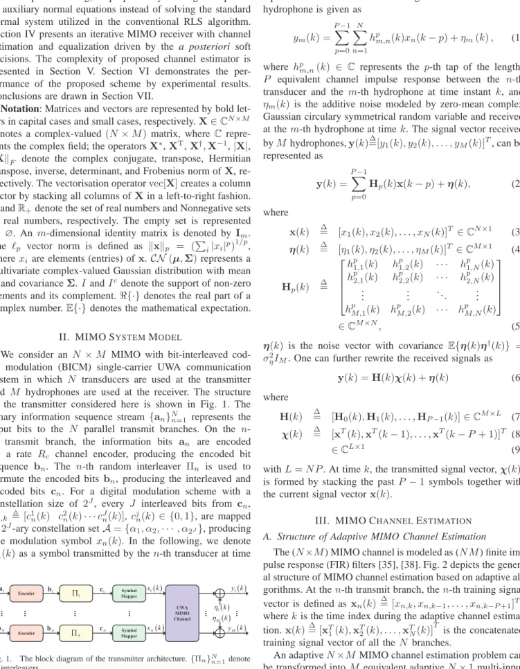
We consider an N ×M MIMO with bit-interleaved cod-ed modulation (BICM) single-carrier UWA communication system in which N transducers are used at the transmitter and M hydrophones are used at the receiver. The structure of the transmitter considered here is shown in Fig. 1. The binary information sequence stream {an}Nn=1 represents the
input bits to the N parallel transmit branches. On the n -th transmit branch, -the information bits an are encoded
by a rate Rc channel encoder, producing the encoded bit sequence bn. The n-th random interleaver Πn is used to
permute the encoded bits bn, producing the interleaved and
encoded bits cn. For a digital modulation scheme with a
constellation size of 2J, every J interleaved bits from c
n,
cn,k ,[c1n(k) c2n(k)· · ·cJn(k)],cjn(k)∈ {0,1}, are mapped
to2J-ary constellation setA={α
1, α2,· · · , α2J}, producing
one modulation symbol xn(k). In the following, we denote
xn(k)as a symbol transmitted by then-th transducer at time
k. Encoder Symbol Mapper 1 Õ Encoder Symbol Mapper N Õ UWA MIMO Channel ... ... ... ... ... ... 1 a N b ( ) 1 x k ( ) N x k ( ) 1 y k ( ) M y k ( ) 1k h ( ) M k h 1 b N a 1 c N c
Fig. 1. The block diagram of the transmitter architecture.{Πn}Nn=1denote N interleavers.
The frequency-selective channel is modeled by a sample-space tapped delay line. We assume that the maximum mul-tipath delay in symbol intervals is at mostP. At time k, the equivalent discrete-time baseband signal received on them-th hydrophone is given as ym(k) = P−1 X p=0 N X n=1 hpm,n(k)xn(k−p) +ηm(k), (1) where hp
m,n(k) ∈ C represents the p-th tap of the length-P equivalent channel impulse response between the n-th transducer and the m-th hydrophone at time instant k, and
ηm(k) is the additive noise modeled by zero-mean complex
Gaussian circulary symmetrical random variable and received at them-th hydrophone at timek. The signal vector received byM hydrophones,y(k)=[y∆ 1(k), y2(k), . . . , yM(k)]T, can be
represented as y(k) = P−1 X p=0 Hp(k)x(k−p) +η(k), (2) where x(k) =∆ [x1(k), x2(k), . . . , xN(k)]T ∈CN×1 (3) η(k) =∆ [η1(k), η2(k), . . . , ηM(k)]T ∈CM×1 (4) Hp(k) =∆ hp1,1(k) h p 1,2(k) · · · h p 1,N(k) hp2,1(k) h p 2,2(k) · · · h p 2,N(k) .. . ... . .. ... hpM,1(k) h p M,2(k) · · · h p M,N(k) ∈CM×N, (5)
η(k) is the noise vector with covariance E{η(k)η†(k)} =
σ2
ηIM. One can further rewrite the received signals as
y(k) =H(k)χ(k) +η(k) (6) where
H(k) =∆ [H0(k),H1(k), . . . ,HP−1(k)]∈CM×L (7)
χ(k) =∆ [xT(k),xT(k−1), . . . ,xT(k−P+ 1)]T (8)
∈CL×1 (9)
withL=N P. At timek, the transmitted signal vector,χ(k), is formed by stacking the pastP −1 symbols together with the current signal vectorx(k).
III. MIMO CHANNELESTIMATION
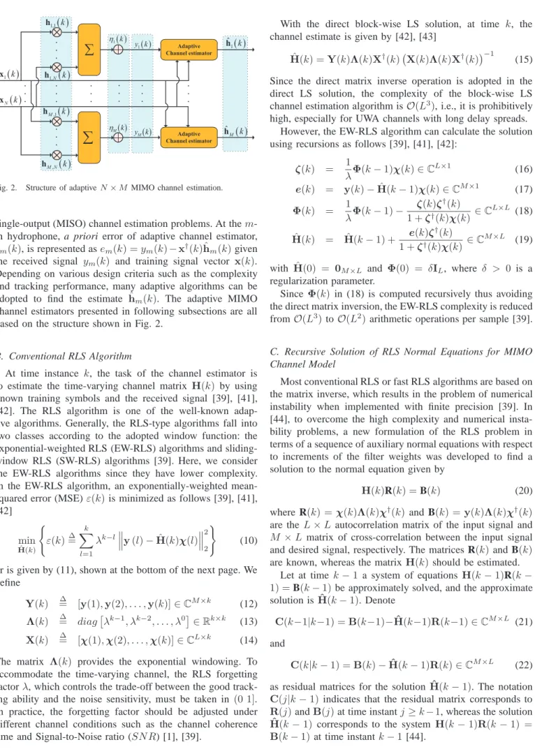
A. Structure of Adaptive MIMO Channel Estimation
The (N×M) MIMO channel is modeled as (N M) finite im-pulse response (FIR) filters [35], [38]. Fig. 2 depicts the gener-al structure of MIMO channel estimation based on adaptive gener- al-gorithms. At then-th transmit branch, then-th training signal vector is defined as xn(k)= [xn,k∆ , xn,k−1, . . . , xn,k−P+1]T,
wherekis the time index during the adaptive channel estima-tion.x(k)= [∆ xT
1(k),xT2(k), . . . ,xTN(k)] T
is the concatenated training signal vector of all theN branches.
An adaptiveN×M MIMO channel estimation problem can be transformed intoM equivalent adaptiveN×1multi-input
Adaptive Channel estimator Adaptive Channel estimator
å
å
. . . . . . . . . . . . . . . . . . ( ) 1 y k ( ) M y k ( ) 1 k h ( ) M k h . . . . . .( )
1 ˆ k h( )
ˆ M k h( )
1 k x( )
N k x( )
1,1 k h( )
1,N k h( )
,1 M k h( )
, M N k hFig. 2. Structure of adaptiveN×M MIMO channel estimation.
single-output (MISO) channel estimation problems. At them -th hydrophone, a priori error of adaptive channel estimator,
em(k), is represented asem(k) =ym(k)−x†(k)ˆhm(k)given
the received signal ym(k) and training signal vector x(k). Depending on various design criteria such as the complexity and tracking performance, many adaptive algorithms can be adopted to find the estimate hˆm(k). The adaptive MIMO channel estimators presented in following subsections are all based on the structure shown in Fig. 2.
B. Conventional RLS Algorithm
At time instance k, the task of the channel estimator is to estimate the time-varying channel matrix H(k) by using known training symbols and the received signal [39], [41], [42]. The RLS algorithm is one of the well-known adap-tive algorithms. Generally, the RLS-type algorithms fall into two classes according to the adopted window function: the exponential-weighted RLS (EW-RLS) algorithms and sliding-window RLS (SW-RLS) algorithms [39]. Here, we consider the EW-RLS algorithms since they have lower complexity. In the EW-RLS algorithm, an exponentially-weighted mean-squared error (MSE) ε(k)is minimized as follows [39], [41], [42] min ˆ H(k) ( ε(k)=∆ k X l=1 λk−l y(l)− ˆ H(k)χ(l) 2 2 ) (10)
or is given by (11), shown at the bottom of the next page. We define Y(k) ∆= [y(1),y(2), . . . ,y(k)]∈CM×k (12) Λ(k) ∆= diag λk−1, λk−2, . . . , λ0 ∈Rk×k (13) X(k) ∆= [χ(1),χ(2), . . . ,χ(k)]∈CL×k (14) The matrix Λ(k) provides the exponential windowing. To accommodate the time-varying channel, the RLS forgetting factorλ, which controls the trade-off between the good track-ing ability and the noise sensitivity, must be taken in (0 1]. In practice, the forgetting factor should be adjusted under different channel conditions such as the channel coherence time and Signal-to-Noise ratio (SN R) [1], [39].
With the direct block-wise LS solution, at time k, the channel estimate is given by [42], [43]
ˆ
H(k) =Y(k)Λ(k)X†(k) X(k)Λ(k)X†(k)−1
(15) Since the direct matrix inverse operation is adopted in the direct LS solution, the complexity of the block-wise LS channel estimation algorithm isO(L3), i.e., it is prohibitively
high, especially for UWA channels with long delay spreads. However, the EW-RLS algorithm can calculate the solution using recursions as follows [39], [41], [42]:
ζ(k) = 1 λΦ(k−1)χ(k)∈C L×1 (16) e(k) = y(k)−Hˆ(k−1)χ(k)∈CM×1 (17) Φ(k) = 1 λΦ(k−1)− ζ(k)ζ†(k) 1 +ζ†(k)χ(k) ∈C L×L (18) ˆ H(k) = Hˆ(k−1) + e(k)ζ †(k) 1 +ζ†(k)χ(k)∈C M×L (19)
with Hˆ(0) = 0M×L and Φ(0) = δIL, where δ > 0 is a
regularization parameter.
Since Φ(k) in (18) is computed recursively thus avoiding the direct matrix inversion, the EW-RLS complexity is reduced fromO(L3)toO(L2)arithmetic operations per sample [39].
C. Recursive Solution of RLS Normal Equations for MIMO Channel Model
Most conventional RLS or fast RLS algorithms are based on the matrix inverse, which results in the problem of numerical instability when implemented with finite precision [39]. In [44], to overcome the high complexity and numerical insta-bility problems, a new formulation of the RLS problem in terms of a sequence of auxiliary normal equations with respect to increments of the filter weights was developed to find a solution to the normal equation given by
H(k)R(k) =B(k) (20)
where R(k) =χ(k)Λ(k)χ†(k) and B(k) = y(k)Λ(k)χ†(k)
are the L×L autocorrelation matrix of the input signal and
M ×L matrix of cross-correlation between the input signal and desired signal, respectively. The matrices R(k)and B(k)
are known, whereas the matrix H(k)should be estimated. Let at time k−1 a system of equationsH(k−1)R(k−
1) =B(k−1)be approximately solved, and the approximate solution is Hˆ(k−1). Denote
C(k−1|k−1) =B(k−1)−Hˆ(k−1)R(k−1)∈CM×L (21)
and
C(k|k−1) =B(k)−Hˆ(k−1)R(k)∈CM×L (22)
as residual matrices for the solution Hˆ(k−1). The notation
C(j|k−1) indicates that the residual matrix corresponds to
R(j)andB(j)at time instantj≥k−1, whereas the solution
ˆ
H(k−1) corresponds to the system H(k−1)R(k−1) =
For the convenience of following derivation, we denote
∆R(k) = R(k)−R(k−1), ∆B(k) = B(k)−B(k −1), and
∆H(k) =H(k)−Hˆ(k−1). (23) With the previously obtained solution Hˆ(k −1) and the residual matrix C(k|k−1), our purpose is to find a solution
ˆ
H(k)of (20). The equation (20) can be rewritten as h
ˆ
H(k−1) + ∆H(k)iR(k) =B(k) (24) Hence, the system of equations with respect to the unknown matrix ∆H(k)is represented as
∆H(k)R(k) =C(k|k−1). (25) Instead of solving the original problem (20), we can find a solution ∆ ˆH(k) of the auxiliary system of equations (25), where
C(k|k−1) =C(k−1|k−1)+∆B(k)−Hˆ(k−1)∆R(k) (26)
and an approximate solution of the original system (20) is obtained as
ˆ
H(k) = ˆH(k−1) + ∆ ˆH(k). (27) For the EW-RLS problem, theL×Lmatrix R(k)andM×L
matrix B(k)can be recursively updated as [39]
R(k) =λR(k−1) +χ(k)χ†(k)∈CL×L, (28)
B(k) =λB(k−1) +y(k)χ†(k)∈CM×L, (29)
where k >0, R(0) =̺IL, and ̺is a small positive number
for regularization of the adaptation at the initial stage. The residual matrix C(k|k−1) in equation (26) can be efficiently updated using the following relationship [44]
C(k|k−1) =λC(k−1|k−1) +e∗(k)χT(k), (30) where e(k) = y(k)−Hˆ(k−1)χ(k) is the M ×1 a priori
estimation error vector.
D. Homotopy RLS-DCD Algorithm for Time-varying MIMO Sparse Channel Estimation
Time-varying multipath UWA communication channels of-ten exhibit sparsity, i.e., the most entries in H(k) are close to zero [45]. With a priori information on the sparsity, some channel estimators can obtain improved performance in terms of channel tracking and computational complexity [20], [23], [37], [38], [45], [46].
Compressive sensing based sparse channel estimation tech-niques [47] are widely used in UWA communications [48], but the prohibitive computational complexity limits their applica-tion in MIMO UWA systems [49]. Recently, many adaptive algorithms have been developed to deal with sparse recovery problems. Unfortunately, most of these adaptive algorithms for UWA channel estimation have either a good performance
but with a high complexity of at least O(L2), e.g. RLS-type
algorithms, or a low complexity of O(L) but with a low performance, e.g. LMS-type algorithms.
Here, we introduce a recently proposed algorithm, named as the exponentially-weighted Homotopy RLS-DCD algorithm [28], and extend it for estimation of time-varying MIMO sparse channels. Assume that the channel is sparse, i.e. the number S of non-zero taps in hp
m,n(k), p = 0,· · · , P −1,
satisfiesS≪P. A sparse approximation to the UWA channel response H(k) can be obtained by solving the following optimization problem: min ˆ H(k) vec h ˆ H(k)i 0, s.t. ε(k)≤ǫ (31)
where ǫ is a small positive constant, which controls the estimation error. The non-convexity of above optimization problem results in intractable computations. A convex relax-ation provides a viable alternative to the non-convex problem, whereby theℓ0-norm,
vec h ˆ H(k)i
0is replaced with theℓ1 -norm
vec h
ˆ
H(k)i
1. Various adaptive filters can solve this problem in a computationally efficient way [50]–[52].
The adaptive filter finds a complex-valued tap-weight matrix
ˆ
H(k), which, at every time instant k, minimizes the cost functionε′(k): min ˆ H(k) ε′(k)∆= 1 σ2ε(k) +fp h ˆ H(k)i , (32)
where the first term of ε′(k) is the LS error of the solution
and the second term fphHˆ(k)i is a penalty function that incorporates a priori information on the solution [52]:
fphHˆ(k)i=τ
w
T(k)vechHˆ(k)i
1 (33)
where the vector w containsM Lpositive weightswj(k)which are updated during the adaptation as [53]
wj(k) = 1
|hj(k−1)|2+ς, (34)
ς >0 is an adjusted parameter,hj(k−1)is thej-th element
in the estimated channel vectorvec( ˆH(k−1)). The positive scalarτ in (33) is a regularization parameter that controls the balance between the LS fitting term and the penalty term in (32).
The Homotopy algorithm minimizes the cost functionε′(k)
in (32). A set of homotopy iterations is performed for exponen-tially decreasing values of the regularization parameter vector
τ:τ ←γτ, whereγis the decreasing factor and must be taken in (0,1). If γ is close to one, a large number of homotopy iterations are needed, which result in a high complexity. In order to reduce the complexity of adaptive filtering based on the Homotopy algorithm, it is enough to perform only one homotopy iteration. For further reduction in the complexity, DCD iterations are used [44], [54].
min ˆ H(k) ε(k)= tr∆ Y(k)−Hˆ(k)X(k)Λ(k)Y(k)−Hˆ(k)X(k)† (11)
TABLE I
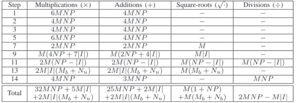
EXPONENTIAL-WEIGHTEDHOMOTOPYRLS-DCDADAPTIVE ALGORITHM FORMIMOCHANNEL ESTIMATION
Input:χ,y,τ,M,L,λ,γ,Mb,Nu,ε Output:Hˆ(k),C(k|k)
Step Initialization:Hˆ(0) =0,{Im=∅}Mm=1,C(0|0) =0,B(0) =0,R(0) =εIL,W(1) =1M×L
fork= 1toK%loop f or K received symbols
1 R(k) =λR(k−1) +χ(k)χ†(k)
2 B(k) =λB(k−1) +y(k)χ†(k)
3 d(k) =Hˆ(k−1)χ(k)
4 e(k) =y(k)−d(k)
5 C(k|k−1) =λC(k−1|k−1) +e∗(k)χT(k)
6 form= 1toM %loop f or M hydrophones
7 τm= maxj|cm,j|,1≤j≤L
8 t= arg minj∈Im 12|hm,j|2Rj,j+ℜ{h∗m,jcm,j} −τmwm,j|hm,j|
9 if 1
2|hm,t|2Rt,t+ℜ{h∗m,tcm,t} −τmwm,t|hm,t|<0
9.1 Remove thet-th element fromIm(Im←Im\t)
9.2 cm(k|k−1) =cm(k|k−1) +hm,tR(t)(k) end if
10 t= arg maxj∈Icm
(|cm,j|−τmwm,j)2
Rj,j
if|cm,t|> τmwm,t
11 Include thet-th element into the support(Im←Im∪t) end if
12 ⊛Update the regularization parameter:τm←γτm
13 ⊛Approximately solve the equation (25) by using the LS-ℓ1optimization on the supportImusing theℓ1-DCD algorithm 14 ⊛Update the weight matrixW(k)using equation (34)
end for end for
In a DCD iteration, the previously obtained solutionHˆ(k−
1) is used as a warm-start for minimizing the cost ε′(k) at
timek. This minimization is equivalent to minimization [52]
1
2∆H(k)R(k)∆H
†(k)− ℜ{C(k|k−1)∆H†(k)} +τ|Hˆ(k)|WT(k)
(35)
with respect to the matrix ∆H(k), where W ∈ RM×L+ is a weight matrix formed by reshaping theM L×1vector w, and
C(k|k−1)is given by (30).
The cost function in (32) is minimized using the leadingℓ1
-DCD algorithm from [28]. In the leadingℓ1-DCD algorithm,
a criterion for terminating computations in every Homotopy iteration is a maximum number of DCD updatesNu. Typically,
Nu is set to a small value for limiting the complexity of the algorithm [44].
Table I shows the EW-HRLS-DCD adaptive algorithm for time-varying MIMO channel estimation, wherecm(k|k−1)is the m-th row of the matrixC(k|k−1),cm,j is thej-th entry of the vectorcm(k|k−1),hm,j is the entry of channel matrix
ˆ
H(k−1)in them-th row andj-th column,wm,j is the entry of weight matrixW(k)in them-th row andj-th column, and
τmis them-th element of vectorτ.
IV. PROPOSEDCE-BASEDSOFTDECISIONTURBO
EQUALIZATION FORMIMOSYSTEMS
In this section, we propose an iterative sparse channel estimation and equalization driven by the a posteriori soft-decision symbols for time-varying MIMO UWA communica-tion system.
The proposed iterative receiver is shown in Fig. 3. It consists of the MIMO MMSE linear equalizer (LE), itera-tive MIMO adapitera-tive channel estimator, soft-input soft-output (SISO) demappers, deinterleavers, SISO mappers, interleavers and MAP decoders. The iterative MIMO adaptive channel estimator provides an estimate of channel matrix, Hˆ, noise covariance vectorσˆ and phase vectorθˆdriven by the training symbolsX, hard decisionQ( ˆX)and a posteriori soft decision
˜
X; the phase vectorθˆis updated by an embedded second-order phase-locked loop (PLL) as used in [1], [45]. The MIMO TEQ applies a MMSE equalizer, and then hard or soft decisions of the equalized symbols are fed to the SISO demappers or the iterative MIMO adaptive channel estimator, respectively. The SISO demappers output the extrinsic information of the transmitted bits {LE
e{cn}}Nn=1, which is then passed to
the de-interleavers and treated as the a priori information
{LD
a{bn}}Nn=1 for the MAP decoder. Finally, the MAP
de-coders output extrinsic information {LD
e{bn}}Nn=1, which is
further fed back to the equalizer as the a priori information
{LE
a{cn}}Nn=1 of the transmitted bits. After several turbo
iterations, the MAP decoders output estimates of transmitted bits{an}Nn=1.
A. Received Signal Model for MIMO Equalization
In the following, we assume the symbol rate sampling. Let
Lf andLp be the length of the noncausal and causal parts of
the equalizer, respectively. In order to perform the equalization and estimate the transmitted symbols at time k, we consider an observation window containingLp+Lf+ 1received signal
1 Õ 1 1 -Õ
{ }
1 D a L b MAP Decoder SISO Demapper SISO Mapper MUX{ }
1 D e L b{ }
1 E a L c{ }
1 E e L c 1 Õ 1 1 -Õ{ }
D a N L b MAP Decoder SISO Demapper SISO Mapper{ }
D e N L b{ }
E a N L c{ }
E e N L c 1 ˆ a ˆN a D EM U X Iterative MIMOAdaptive Channel Estimator MIMO MMSE LE ... ... ... ... ˆ H
σ
ˆ
X X Training Symbols X ˆ XΣ
X or or( )
ˆ Q X ˆ θ 1 y M y ... ...Fig. 3. Block diagram of iterativeN×M MIMO receiver coupled with adaptive sparse channel estimator.
be written as [20], [56]
rk=Hksk+nk (36)
where Hk is given by (37), shown at the bottom of the next
page, and rk = yT(k+Lf),· · ·,yT(k− Lp) T , (38) sk = xT(k+Kf+Lf),· · · ,xT(k− Kp− Lp) T , (39) nk = ηT(k+Lf),· · · ,ηT(k− Lp) T . (40)
The channel length is P =Kp+Kf + 1, whereKf andKp
are the length of precursor and postcursor parts of the channel response, respectively. For convenience, we will denote K= N(Kp+Kf+Lp+Lf + 1)the overall length of the vector
sk andL=M(Lp+Lf+ 1)the overall length of the vector
rk. The noise vectornk is assumed to be zero-mean complex
Gaussian, i.e.,nk∼ CN(0, σ2nIL). TheHkis a block channel
matrix made up of Hp(k) defined in (5), hence, the size of
Hk becomesL × K.
B. Linear MMSE Turbo Equalization
In practice, the channel impulse responses have to be estimated and then are used to calculate the coefficients of the TEQ. We denote Hˆk and Ek = Hk −Hˆk the channel
estimate and the corresponding channel estimation error, re-spectively. Let us assume that Ek has zero mean and it is
uncorrelated with Hˆk andsk. Hence, we can rewrite (36) as
rk = ˆHksk + (Eksk +nk). Given Hˆk, the linear MMSE
estimate ofxn(k)is obtained from [20], [38], [56]
ˆ xn(k) = ˆfn†(k)rk−Hˆksn(k) , (41) ˆ fn(k) = ˆ HkΣn,kHˆk†+σw2IL −1 ˆ hn(k), (42) where sn(k) = xT(k+Kf+Lf),· · · ,xT(k−1),xˇTn(k), xT(k+ 1),· · ·,xT(k− Kp− Lp) T , (43) x(k) = [¯x1(k),x¯2(k),· · · ,xN¯ (k)]T, (44) Σn,k = diag(vn,1,· · · , vn,k−1,1, vn,k+1,· · ·, vn,K), (45) ˇ xn(k) = [¯x1(k),· · · ,xn−¯ 1(k),0,xn¯ +1(k),· · · , ¯ xN(k)]T, (46)
and where x(k) is a priori mean vector of x(k), and Σn,k
is the a priori covariance matrix of x(k). The vector hˆn(k)
is the (N(Lp +P −1) +n)-th column of Hˆk. Hence, we
can obtainxn(k)¯ andvn,k from a priori log-likelihood ratios (LLRs) as in [56] ¯ xn(k) = E(xn(k)) =∆ X αi∈A αi·P(xn(k) =αi), (47) vn,k =∆ Cov(xn(k), xn(k)) = X αi∈A |αi|2·P(xn(k) =αi))− |xn¯ (k)|2, (48) where P(xn(k) =αi) = J Y j=1 P(cjn(k) =si,j), = J Y j=1 1/2· 1 +˜si,j·tanh(LE a(cjn(k)/2) , (49)
the bit patternsi ∆
= [si,1, si,2,· · · , si,J] corresponds toαi ∈
A, and ˜ si,j=∆ ( +1, si,j= 0 −1, si,j= 1 . (50)
The extrinsic LLR for cj
n(k) is given by (51), shown at the
bottom of the next page, whereµn(k) = ˆˆ fH
n (k)ˆhn(k), andA0j
andA1
j are the set of all constellation points such thatsi,j is
C. A Posteriori Soft Decision
After first equalization, the a posteriori soft decisionxn(k)˜
of the equalized symbolxn(k)ˆ is available and can be calcu-lated as [27], [37] ˜ xn(k) = X αi∈A αiP xn(k) =αi|xn(k)ˆ (52) where P xn(k) =αi|ˆxn(k)
is the a posteriori probability
of xn(k) and is given by (53), shown at the bottom of the
next page.P(xn(k) =αi)is the a priori probability and can be calculated with the a priori LLRs from the MAP decoder as in (49), and p(ˆxn(k))is computed with the normalization P2q
i=1P
xn(k) =αi|xn(k)ˆ
= 1. Under the assumption of the Gaussian distribution as in [56], the equalizer outputxn(k)ˆ
conditioned onxn(k) =αi is given by:
p(ˆxn(k)|xn(k) =αi) = 1 πδ˜2 n exp −|xn(k)ˆ −xn˜ (k)αi| 2 ˜ δ2 n , (54) where the a posteriori variance of xn(k)is obtained as
˜ δ2n= 2Q X i=1 |αi−xn(k)˜ |2P xn(k) =αi|xnˆ (k) . (55)
Over the turbo iterations, the reliability of the a posteriori soft decisionxn(k)˜ increases thus improving the accuracy of channel estimation and also speeding up the convergence of the channel estimator.
D. A Posteriori Soft Decision Driven Homotopy RLS-DCD Algorithm
In the iterative channel estimation based on adaptive filter-ing, the adaptive filter is driven by the decision errore(k). The adaptive channel estimation algorithm aims to minimize the variance of the decision errors, so the reliability of the decision plays a very important role in the adaptive channel estimation. In practice, the adaptive channel estimator generally works under two modes: the training mode and direct-decision mode. According to the mode, we can define three types of decision error as following [58] e(k) = y(k)−Hˆ(k−1)χ(k)∈CM×1, (56) ˆ e(k) = y(k)−Hˆ(k−1)Q( ˆχ(k))∈CM×1, (57) ¯ e(k) = y(k)−Hˆ(k−1) ¯χ(k)∈CM×1, (58)
where χ(k) presents the perfect decision corresponding to the training mode. The vector χ¯(k)consists of a priori soft decisions of transmitted symbols under the direct-decision mode, andQ( ˆχ(k))denotes the hard decision of the equalizer output, χˆ(k). In what follows, the vectors e(k), e¯(k) and
ˆ
e(k) are named the perfect decision error vector, a priori soft decision error vector and hard decision error vector, respectively.
In existing iterative adaptive channel estimation algorithms, the hard decision or a priori soft decision symbols are used for driving the estimator. In [27], [37], an efficient adaptive turbo equalizer is proposed, where the more reliable a posteriori soft decisions are used in the adaptive update of the channel coefficients and for the MMSE equalizer. In order to reduce the complexity of the adaptive turbo equalization, the equalizer fil-ter coefficients are adaptively updated via the normalized LMS (NLMS) [39] or the IPNLMS [24] algorithm. The DA-TEQ scheme with the a posteriori soft decisions achieves faster convergence and higher spectrum efficiency than schemes with hard decision or with a priori soft decision. Inspired by [37], here, we use the a posteriori soft decisions to drive the channel estimator. For convenience, we define the a posteriori decision error vector as
˜
e(k) =y(k)−Hˆ(k−1) ˜χ(k)∈CM×1 (59) where χ˜(k) is the a posteriori soft decision vector of the equalizer outputχˆ(k).
The proposed iterative channel estimator comprises the following two stages:
1) Training Stage: The known training symbols xn(k)
within the training symbol vector χ(k) are used to estimate the channel impulse response.
2) Direct-Decision Stage: There are no known training
symbols available at this stage. The hard-decisions of the equalizer output xn(k)ˆ are usually used for tracking the channel. However, the hard-decision is not reliable, leading to error decisions on the transmitted symbols. Hence, the decision errors will cause the error propagation, which can be catastrophic for turbo equalization. Iterative channel estimators in turbo equalization schemes mostly employ the hard-decision or a priori soft decisions at the direct-decision stage. At the initial stage of turbo equalization, the a priori or a posteriori soft-decision from the decoder or equalizer is not yet available, thus we use hard-decisions of the equalizer output as training symbols for the channel estimation. In subsequent iterations, the a posteriori soft decisions, which possess higher reliability than the a priori soft decisions, are utilized.
Hk= Hp−Kf(k+Lf) · · · Hp−Kp(k+Lp) 0 0 0 . .. · · · . .. 0 0 0 Hp+Kf(k− Lp) · · · Hp+Kp(k− Lp) , (37) LEe cjn(k) = ln P θ∈A0 jexp −|xˆn(k)−µˆn(k)θ|2 ˆ µn(k)(1−µˆn(k)) + 1 2 PJ i=1,i6=j˜si,jLEa(cin(k)) P θ∈A1 jexp −|xˆn(k)−µˆn(k)θ|2 ˆ µn(k)(1−µˆn(k)) + 1 2 PJ i=1,i6=j˜si,jLEa(cin(k)) (51)
E. A Posteriori Soft Decision Driven Turbo Equalization
The quality of the soft decision plays a very important role in the performance of the MMSE equalizer. The a priori soft decisions are adopted in many adaptive turbo equalization schemes [21], [22], [57]. With the more reliable a posteriori soft decisions, performance of MMSE equalizer can be im-proved [37]. The output of a posteriori soft decision driven equalizer, xn(k)ˆ , is obtained as
ˆ
xn(k) = ˆfnH(k)rk−Hˆk˜sn(k)
(60) Here, we utilized the a posteriori soft decisions ˜sn(k) =
˜ xT(k+K f+Lf),· · · ,˜xT(k−1), ~xTn(k),x˜T(k+ 1),· · ·, ˜ xT(k− Kp− Lp) T
instead of the a priori soft decisions
¯
sn,k in (41), where x˜(k) = [˜x1(k),x˜2(k),· · ·, xN˜ (k)]T
when k′ 6= k for k′ ∈ [k − Kp − Lp, k +Kf + Lf],
and~xn(k) = [˜x1(k),· · ·,xn−˜ 1(k),0,˜xn+1 (k),· · ·,xN˜ (k)]T
when k′ =k; obviously,xn˜ (k)is excluded for avoiding self cancellation [37].
V. COMPLEXITYCOMPARISON FORMIMO CHANNEL
ESTIMATORS
In this section, the complexity of two channel estimators, EW-RLS and EW-HRLS-DCD, is compared. The algorithm complexity is evaluated in terms of the number of real-valued multiplications, additions, square-root, and division operations per time sample.
The work [28] details the complexity of the EW-HRLS-DCD algorithm for SISO system. According to the general structure of adaptive MIMO channel estimator as shown in Fig. 2, the N ×M MIMO system can be treated as M
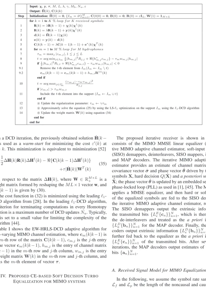
SISO systems with a channel length of L = N P each. Hence, the complexity of the EW-HRLS-DCD algorithm for MIMO system can be easily calculated by following steps in [28] for a SISO system. We can approximately estimate the complexity of the channel estimator based on the EW-HRLS-DCD algorithm for a MIMO system as presented in Table II. In Table I, step 13 requires using the leading ℓ1-DCD
algorithm, where Mb is the number of bits used for repre-sentation of entries in the solution vector, this defining the accuracy of the fixed-point representation [44], and Nu is a maximum number of DCD iterations. The update of the vector
cm(k|k−1) in the leading ℓ1-DCD algorithm is the most
consuming part of the algorithm. The details of the involving computation of the leading ℓ1-DCD algorithm are found in
Table II in [28], and the reader is referred to detail [52]. In overall, as shown in Table II, the EW-HRLS-DCD algorithm requires about32M N P+5M|I|+2M|I|(Mb+Nu)
real-valued multiplications,25M N P+ 2M|I|+ 2M|I|(Mb+ Nu)real-valued additions,M(1+N P)+M(Mb+Nb) square-root operations, and 2M N P −M|I|real-valued divisions.
For comparison, arithmetic operations in the conventional EW-RLS algorithm described by equations (16)-(19) are listed
in Table III. The overall complexity of the conventional EW-RLS algorithm roughly requires 12(N P)2+ 8M N P
real-valued multiplications, 9(N P)2+ 6M N P +M real-valued
additions, and (2M+ 2N P+ 1)N P real-valued divisions. For first example, for N = 2, M = 8,P = 40, K = 6,
Nu = 4, Mb = 15, and assuming that |I| =K, we obtain that the EW-HRLS-DCD algorithm from [52] requires about
23×103multiplications,18×103additions,800square-root
operations, and1.2×103divisions per time index. The same
figures for the EW-RLS algorithm are80×103,61×103,0,
and 14×103, respectively. Thus, compared to the EW-RLS
algorithm, the EW-HRLS-DCD algorithm reduces the number of multiplications by about3.5times, the number of additions by about3.4 times, and the number of divisions by about 11
times.
For another example with the parameter setup the same as in the first example except for the length of channelP, which is nowP = 100, the EW-HRLS-DCD algorithm requires about
53×103multiplications,42×103additions,1.8×103
square-root operations, and 3.2×10³ divisions per time index. The
same figures for the EW-RLS algorithm are490×103,370× 103, 0, and 83×103, respectively. Thus, compared to the
EW-RLS algorithm, the EW-HRLS-DCD algorithm reduces the number of multiplications by about 9 times, the number of additions by about9times, and the number of divisions by about26 times.
VI. EXPERIMENTALRESULTS
In this section, we evaluate the performance of a receiver with the proposed soft-decision-driven sparse channel estima-tion and turbo equalizaestima-tion scheme and compare it to other receivers.
A. Experimental Environment
The experiment was conducted in the Songhua Lake, Jilin province, China (SHLake2013) on Nov. 2013. The lake depth at the experimental site is 48.6m. Two transducers (antennas) were deployed off a small boat and submerged at about 5 m and 6 m below the surface, respectively. During the experiment, the small boat was drifting with an approximate maximum speed of0.25m/s. The receive vertical linear array of 48 hydrophones was moored with the first hydrophone (closest to the lake bottom) at about 7 m above the lake bottom, and other hydrophones evenly spaced by 0.25m. The communication range was about 2.1 km at the start of the experiment.
B. Signaling and Data Structure
For MIMO transmission, two concurrent data streams with the BICM horizontal encoding scheme were transmitted by using two transducers. The input bits were encoded by a
P xn(k) =αi|xn(k)ˆ = p(ˆxn(k)|xn(k) =αi) p(ˆxn(k)) P(xn(k) =αi). (53)
TABLE II
COMPUTATIONALCOMPLEXITY OFTHEEW-HRLS-DCD CHANNELESTIMATOR
Step Multiplications (×) Additions (+) Square-roots (√·) Divisions (÷)
1 6M N P 4M N P − − 2 4M N P 4M N P − − 3 4M N P 4M N P − − 5 6M N P 4M N P − − 7 2M N P 2M N P M − 9 M(4N P+ 7|I|) M(2N P+ 4|I|) M|I| − 11 2M(N P− |I|) 2M(N P− |I|) M(N P− |I|) M(N P− |I|) 13 2M|I|(Mb+Nu) 2M|I|(Mb+Nu) M(Mb+Nu) − 14 4M N P 3M N P − M N P Total 32M N P+ 5M|I| 25M N P+ 2M|I| M(1 +N P) +2M|I|(Mb+Nu) +2M|I|(Mb+Nu) +M(Mb+Nb) 2M N P−M|I| TABLE III
COMPUTATIONALCOMPLEXITY OFTHEEW-RLS CHANNELESTIMATOR
Equation Multiplications (×) Additions (+) Square-roots (√·) Divisions (÷)
(15) 4(N P)2 3(N P)2 − N P (16) 4M N P 3M N P+M − − (17) 8(N P)2 6(N P)2 − 2(N P)2 (18) 4M N P 3M N P − 2M N P Total 12(N P)2 + 8M N P 9(N P)2 + 6M N P+M − (2M+ 2N P+ 1)N P BPSK Packets 12 packets x 8000 symbols QPSK Packets 12 packets x 8000 symbols 8PSK Packets 12 packets x 8000 symbols 16QAM Packets 12 packets x 8000 symbols Tx1 m seq. Payload Down Chirp Gap Gap 350ms 200ms 511 8000 150ms Packet1: 15s Silent Packet3: 15s ... Up Chirp m seq. Payload Gap Gap Down Chirp Up Chirp Silent Silent Silent m seq. Payload Down Chirp Gap Gap Packet2: 15s Silent Up Chirp m seq. Payload Gap Gap Down Chirp Up Chirp Silent Silent Silent BPSK Packets 12 packets x 8000 symbols QPSK Packets 12 packets x 8000 symbols 8PSK Packets 12 packets x 8000 symbols 16QAM Packets 12 packets x 8000 symbols Tx2 ... 200ms 500ms 500ms ... 350ms 511 8000 500ms 200ms 150ms 500ms 200ms
Fig. 4. The structure of the data streams in a two-transducer transmission in the SHLake2013 experiment.
rate Rc = 1/2 convolutional coder with generator polyno-mial [171, 133] in octal format. The carrier frequency was
fc= 3kHzand the symbol rate was2 ksymbols per second (ksps). The pulse shaping filter was a square-root raised cosine filter with a roll-off factor of0.2[40], leading to an occupied channel bandwidth of about2.4kHz. The sampling rate was
25 kHzat the receiver end.
The data structure of the two data streams and relevant pa-rameters are shown in Fig. 4. Preamble up-chirp and postamble down-chirp, Doppler-insensitive waveforms, were added be-fore and after the data burst for coarse frame synchronization and estimation of an average Doppler shift over the whole data burst. In order to reduce the co-channel interference, two Gold sequences of length 511, Doppler-sensitive waveforms, generated from preferred pairs ofm-sequences [40] and added before and after the data payload were used for coarse frame synchronization and initial estimation of channel parameter-s [40]. Following the frame parameter-synchronization parameter-signal iparameter-s one data packet (payload) with various modulation formats. Only data with QPSK, 8PSK and 16QAM modulations are used for performance evaluation, since the detection performance
is very good with the BPSK modulation. The payload is separated from the m-sequence and up-chirp or down-chirp signal by the gap with the duration 150ms for avoiding the inter-block interference. The length of each payload is 8000 symbols between two gaps. Each burst packet is transmitted every 15 s. The entire duration of data transmission is 12 minutes. The approximate SNR, which is estimated by using the signal part and silent part of received signal, is in the range of 20 dB to 32 dB.
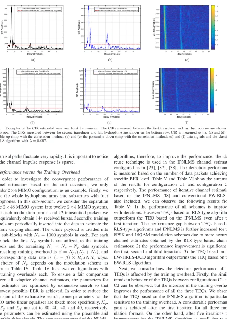
In order to show characteristics of the UWA channel during the experiment, we use the conventional EW-RLS algorithm to estimate the channel impulse response (CIR) over 8000 symbols with QPSK modulation as an example. In Fig. 5, the CIR between the first transducer and last hydrophone (near the surface) is shown in Fig. 5(a). Fig. 5(b) shows the CIR between the second transducer and last hydrophone estimated by using the matched filter applied to the preamble and postamble chirp signals. In Fig. 5, we can observe that the channel multipath spread is about16∼20ms, corresponding to a channel length of 32 ∼40 taps in terms of the symbol rate Rs = 2 ksps. There are three clusters with high energy in the delay domain.
0 10 20 30 40 50 60 70 Delay (Symbols) 100 200 300 400 500 600 700 CIR Amplitude
Channel Estimated using Preamble LFM Threshold amplitude with 1/10 of the main tap magnitude
(a) 0 10 20 30 40 50 60 70 Delay (Symbols) 100 200 300 400 500 600 CIR Amplitude
Channel Estimated using Postamble LFM Threshold amplitude with 1/10 of the main tap magnitude
(b) 10 20 30 40 50 60 70 80 delay/symbols 500 1000 1500 2000 2500 3000 3500 4000 4500 5000 Geo-time/symbols 0.2 0.4 0.6 0.8 1 1.2 1.4 1.6 1.8 (c) 0 10 20 30 40 50 60 70 Delay (Symbols) 100 200 300 400 500 600 700 800 900 1000 1100 CIR Amplitude
Channel Estimated using Preamble LFM Threshold amplitude with 1/10 of the main tap magnitude
(d) 0 10 20 30 40 50 60 70 Delay (Symbols) 100 200 300 400 500 600 700 800 900 1000 CIR Amplitude
Channel Estimated using Postamble LFM Threshold amplitude with 1/10 of the main tap magnitude
(e) 10 20 30 40 50 60 70 80 delay/symbols 500 1000 1500 2000 2500 3000 3500 4000 4500 5000 Geo-time/symbols 0.5 1 1.5 2 2.5 (f)
Fig. 5. Examples of the CIR estimated over one burst transmission. The CIRs measured between the first transducer and last hydrophone are shown on
the top row. The CIRs measured between the second transducer and last hydrophone are shown on the bottom row. CIR is measured using: (a) and (d) the preamble up-chirp with the correlation method; (b) and (e) the postamble down-chirp with the correlation method; (c) and (f) data signals and the classical
EW-RLS algorithm withλ= 0.997.
The arrival paths fluctuate very rapidly. It is important to notice that the channel impulse response is sparse.
C. Performance versus the Training Overhead
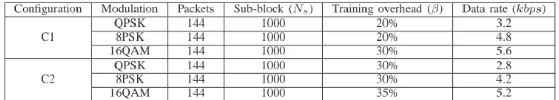
In order to investigate the convergence performance of channel estimators based on the soft decisions, we only consider2×4MIMO configuration, as an example. Firstly, we divide the whole hydrophone array into sub-arrays with four hydrophones. In this sub-section, we consider the separation of the2×48MIMO system into twelve2×4MIMO systems, so for each modulation format and 12 transmitted packets we can equivalently obtain 144 received bursts. Secondly, training symbols are periodically inserted into the data to estimate the fast time-varying channel. The whole payload is divided into eight sub-blocks with Ns= 1000symbols in each. For each sub-block, the first Np symbols are utilized as the training symbols and the remaining Nd = Ns−Np data symbols. The resulting training overhead is β =Np/(Np+Nd), and the corresponding data rate is (1 −β) ×RsJN Rc kbps. The choice of Np depends on the modulation scheme as shown in Table IV. Table IV lists two configurations with two training overheads each. To ensure a fair comparison between all adaptive channel estimators, the parameters for each estimator are optimized by exhaustive search so that the lowest possible BER is achieved. In order to reduce the dimension of the exhaustive search, some parameters for the MIMO turbo linear equalizer are fixed; more specifically,Kp,
Kf, Lp and Lf are set to 80, 40, 40, and 40, respectively.
These parameters can be estimated using the preamble and postamble chirp signals. The convergence speed of the NLMS-type algorithms is much slower than that of the RLS-NLMS-type
algorithms, therefore, to improve the performance, the data reuse technique is used in the IPNLMS channel estimator configured as in [23], [37], [38]. The detection performance is measured based on the number of data packets achieving a specific BER level. Table V and Table VI show the summary of the results for configuration C1 and configuration C2, respectively. The performance of iterative channel estimation based on the IPNLMS [38] and conventional EW-RLS is also included. We can observe the following results from Table V: 1) the performance of all schemes is improved with iterations. However TEQs based on RLS-type algorithms outperform the TEQ based on the IPNLMS even after the first iteration. The performance gap between TEQs based on RLS-type algorithms and IPNLMS is further increased for the 8PSK and 16QAM modulation schemes due to more accurate channel estimates obtained by the RLS-type based channel estimators; 2) the performance improvement is significant at the first, second and third iterations; 3) the TEQ based on the EW-HRLS-DCD algorithm outperforms the TEQ based on the EW-RLS algorithm.
Next, we consider how the detection performance of the TEQs is affected by the training overhead. Firstly, the similar trends in behavior of the TEQs between configurations C1 and C2 can be observed, but the increase in the training overhead improves the performance of all the three TEQs. We observe that the TEQ based on the IPNLMS algorithm is particularly sensitive to the training overhead. A considerable performance gain is achieved after the first iteration for all three mod-ulation formats. On the other hand, after five iterations the improvement for the IPNLMS algorithm is small due to the slow convergence and limited by the fast time-varying channel
TABLE IV
RECEIVERCONFIGURATIONS FOR THEANALYSIS OFCONVERGENCEPERFORMANCE
Configuration Modulation Packets Sub-block (Ns) Training overhead (β) Data rate (kbps)
C1 QPSK 144 1000 20% 3.2 8PSK 144 1000 20% 4.8 16QAM 144 1000 30% 5.6 C2 QPSK 144 1000 30% 2.8 8PSK 144 1000 30% 4.2 16QAM 144 1000 35% 5.2 TABLE V
TOTAL NUMBER OF PACKETS ACHIEVING THE SPECIFIEDBERLEVEL FOR CONFIGURATIONC1
# of Iter. QPSK (BER = 0) 8PSK (BER∈[0,10−
4
]) 16QAM (BER∈[0,10−3])
IPNLMS RLS HRLS-DCD IPNLMS RLS HRLS-DCD IPNLMS RLS HRLS-DCD
0 0 0 0 0 0 0 0 0 0 1 27 63 83 3 13 52 1 16 42 2 68 98 110 8 39 87 2 33 71 3 83 105 134 10 42 97 4 43 84 4 83 105 134 13 50 104 5 47 92 5 86 108 136 14 51 108 6 47 92 TABLE VI
TOTAL NUMBER OF PACKETS ACHIEVING THE SPECIFIEDBERLEVEL FOR CONFIGURATIONC2
# of Iter. QPSK (BER = 0) 8PSK (BER∈[0,10−
4
]) 16QAM (BER∈[0,10−3])
IPNLMS RLS HRLS-DCD IPNLMS RLS HRLS-DCD IPNLMS RLS HRLS-DCD
0 0 0 0 0 0 0 0 0 0 1 60 79 124 7 35 71 14 31 60 2 84 92 132 14 57 105 21 46 80 3 90 105 132 18 64 120 23 50 84 4 96 113 141 20 71 122 25 50 93 5 97 113 141 20 72 123 26 51 93
(i.e. shorter channel coherence time). For example, the final number of the packets with zero BER increases from 86 to 97 after five iterations for the QPSK modulation. With the RLS-type based channel estimators for all modulation formats as shown in Table VI, there is some increase in the number of packets that achieve the target BER by increasing the number of training symbols.
Fig. 6 details the demodulation results. As shown in the fig-ure, the EW-HRLS-DCD based TEQ can successfully retrieve the 141 data packets out of 144 packets for the QPSK mod-ulation. This implies that our proposed receiver can achieve a data rate of 3.2 kbps with a low error probability. On the other hand, for the 8PSK case, with our receiver and 20%
training overhead, there are 122 packets with BER <10−4,
there are 137 packets with BER <10−4 when 30% training
overhead is used. Note that for the 16QAM modulation, the large performance gain can be observed in terms of the total number of the packets with BER <10−2.
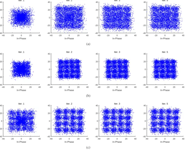
The constellation diagram is a useful tool to demonstrate the reliability of the received and equalized symbols. The evolutional behavior of the equalized and a posteriori soft-decision symbols in terms of constellation diagram are shown in Fig. 7 and Fig. 8, respectively. Results for the 16QAM modulation in the four iterations are only presented. In Fig. 7, for the channel estimator based on the IPNLMS algorithm, the improvement in the quality of the equalized symbols with iterations is little, while the improvement in quality obtained by RLS-type channel estimators is more considerable. On the other hand, compared to the RLS channel estimator, the
EW-HRLS-DCD channel estimator can achieve better quality of equalized symbols with more iterations.
Fig. 8 shows the evolution of the a posteriori soft-decision symbols. What is interesting to observe is that the soft-decision symbols in all the three schemes can almost converge to the ideal constellation points. For schemes based on RLS and EW-HRLS-DCD channel estimators, these results are consistent with the results shown in Fig. 7(b) and Fig. 7(c). From Fig. 7(a), it is however difficult to recognize the modulation scheme even after five iterations. Obviously, the result shown in Fig. 8(a) is a counterintuitive from the observation in Fig. 7(a). This appears due to inaccurate channel estimation provided by the IPNLMS algorithm, which is catastrophic for turbo equalization. The a posteriori soft-decision evaluated from the equalizer based on the IPNLMS channel estimator converges to the wrong constellation points due to the error propagation incurred by inaccurate channel estimates. With a high quality of channel estimation as shown in Fig. 8(b) and Fig. 8(c), the a posteriori soft-decision symbols are more reliable than equalized symbols due to accurate channel estimates and the usage of the soft decoder. However, with inaccurate channel estimates, the a posteriori soft-decision symbols convergence to wrong constellation points due to the error propagation in turbo iteration procedure as shown in Fig. 8(a).
D. Performance versus MIMO size
Table VII shows three configurations of MIMO system used to demonstrate the effect of the MIMO size on the
-40 -20 0 20 40 In-Phase -40 -20 0 20 40 Quadrature Iter. 1 -40 -20 0 20 40 In-Phase -40 -20 0 20 40 Iter. 2 -40 -20 0 20 40 In-Phase -40 -20 0 20 40 Iter. 3 -40 -20 0 20 40 In-Phase -40 -20 0 20 40 Iter. 5 (a) -40 -20 0 20 40 In-Phase -40 -20 0 20 40 Quadrature Iter. 1 -40 -20 0 20 40 In-Phase -40 -20 0 20 40 Iter. 2 -40 -20 0 20 40 In-Phase -40 -20 0 20 40 Iter. 3 -40 -20 0 20 40 In-Phase -40 -20 0 20 40 Iter. 5 (b) -40 -20 0 20 40 In-Phase -40 -20 0 20 40 Quadrature Iter. 1 -40 -20 0 20 40 In-Phase -40 -20 0 20 40 Iter. 2 -40 -20 0 20 40 In-Phase -40 -20 0 20 40 Iter. 3 -40 -20 0 20 40 In-Phase -40 -20 0 20 40 Iter. 5 (c)
Fig. 7. Constellation diagrams of the equalized symbols for one burst. Five iterations are conducted with the iterative channel estimation algorithm: (a)
IPNLMS; (b) RLS; (c) EW-HRLS-DCD.
TABLE VII
RECEIVERCONFIGURATIONS FOR THEANALYSIS OFCONVERGENCEPERFORMANCE
MIMO (N×M) Modulation Packets Sub-block (Ns) Training overhead (β) Data rate (kbps)
2×4 QPSK 144 1000 20% 3.2 8PSK 20% 4.8 16QAM 30% 5.6 2×8 QPSK 72 1000 20% 3.2 8PSK 20% 4.8 16QAM 30% 5.6 2×12 QPSK 48 1000 20% 3.2 8PSK 20% 4.8 16QAM 30% 5.6
receiver performance. The 2×48 MIMO system is grouped into multiple smaller MIMO systems according to the number of hydrophones, leading to 144, 72 and 48 received packets for the 2×4,2×8and2×12MIMO setups, respectively.
In Fig. 9 it can be seen that with the QPSK modulation, all the MIMO receivers can achieve perfect data recovery with eight or twelve hydrophones after five turbo iterations.
For the 8PSK modulation, the IPNLMS-based MIMO re-ceiver improves the performance with more hydrophones, but it cannot achieve the zero BER performance. The main reason is that the demodulation for a higher modulation order requires a higher accuracy of channel estimation, which cannot be provided by the IPNLMS algorithm. However, the zero-BER detection is achieved by MIMO receivers with both
RLS-and EW-HRLS-DCD-based channel estimators, in the2×12
configuration.
In Fig. 9(c), detection results are shown for the 16QAM modulation. Generally, the performance of all channel estima-tors keeps improving with more hydrophones. For the2×8
MIMO setup, 2, 8 and 12 error free packets of 72 packets are received with IPNLMS, RLS and EW-HRLS-DCD based receiver, respectively. There are 36, 59 and 64 data packets out of 72 packets with BER < 10−2 for these estimators,
respectively. With the 2×12 MIMO configuration, there are 33, 46 and 48 data packets out of 48 packets with BER<10−2
-1 -0.5 0 0.5 1 In-Phase -1 -0.5 0 0.5 1 Quadrature Iter. 1 -1 -0.5 0 0.5 1 In-Phase -1 -0.5 0 0.5 1 Iter. 2 -1 -0.5 0 0.5 1 In-Phase -1 -0.5 0 0.5 1 Iter. 3 -1 -0.5 0 0.5 1 In-Phase -1 -0.5 0 0.5 1 Iter. 5 (a) -1 -0.5 0 0.5 1 In-Phase -1 -0.5 0 0.5 1 Quadrature Iter. 1 -1 -0.5 0 0.5 1 In-Phase -1 -0.5 0 0.5 1 Iter. 2 -1 -0.5 0 0.5 1 In-Phase -1 -0.5 0 0.5 1 Iter. 3 -1 -0.5 0 0.5 1 In-Phase -1 -0.5 0 0.5 1 Iter. 5 (b) -1 -0.5 0 0.5 1 In-Phase -1 -0.5 0 0.5 1 Quadrature Iter. 1 -1 -0.5 0 0.5 1 In-Phase -1 -0.5 0 0.5 1 Iter. 2 -1 -0.5 0 0.5 1 In-Phase -1 -0.5 0 0.5 1 Iter. 3 -1 -0.5 0 0.5 1 In-Phase -1 -0.5 0 0.5 1 Iter. 5 (c)
Fig. 8. Constellation diagrams of the a posteriori soft-decision symbols for one burst. Five iterations are conducted with the iterative channel estimation
algorithm: (a) IPNLMS; (b) RLS; (c) EW-HRLS-DCD.
E. Comparison between Hard-decision and Soft-decision driv-en Turbo Equalization
As shown in many research works [20], [23], [31], [37], [38], [57], [58], the quality of the output of turbo equalizer with high order modulation is very sensitive to the channel es-timation errors or misadjustment errors produced by a specific adaptive algorithm. On the other hand, the hard decision of the equalizer output detriments the quality of channel estimation and MMSE equalizer due to the error propagation.
Since the true CIRs are not known for the experimental data processing, we can not evaluate the accuracy of channel estimation with various feedback information in terms of MSE. In order to quantify the performance gain brought by channel estimators with different feedback, in [21], the behavior of turbo receiver was investigated in terms of decision-directed mean squared error (DD-MSE) at the output of equalizer ver-sus the number of iterations. The DD-MSE can be estimated adaptively as follows [21], [37]:
εkMSE+1 =γεkMSE+ (1−γ)|ek|2, (61)
where the forgetting factor γ is set to 0.99. The error ek can be replaced by ˆe(k), ¯e(k), ore(k)˜ corresponding to the hard decision error, a priori soft decision error, or a posteriori soft decision error defined as in (57), (58) and (59), respectively. It is noted that ek is replaced by the hard decision error due
to unavailable a priori information from decoder at the initial turbo iteration.
From the analysis in the previous subsections, with a small MIMO size, the TEQs based on the IPNLMS algorithm experience problems for high order modulation due to the error propagation. Therefore, the comparison between the proposed TEQ and the hard decision based TEQ is limited to the2×8
MIMO with 8PSK modulation. In addition, we only choose those packets, which do not experience convergence problem by using all the three channel estimators, for fair benchmark in following analysis.
Fig. 10 depicts the DD-MSE for the three channel estimators and for the hard-decision and a posteriori SD feedback. Clearly, for all the estimators, the TEQ with the a posteriori SD outperforms that with the hard-decisions. With the a
poste-riori SD, the IPNLMS based channel estimator approximately
obtains4dBDD-MSE gain, the RLS based channel estimator approximately obtains 7 dB DD-MSE gain, the EW-HRLS-DCD based channel estimator approximately obtains 7 dB
DD-MSE gain with respect to that with the hard-decision feedback. On the other hand, comparison of the three channel estimators shows that the smallest DD-MSE is achieved by the EW-HRLS-DCD algorithm with the a posteriori SD.
Finally, Fig. 11 demonstrates the performance of TEQs with three channel estimators versus the number of turbo
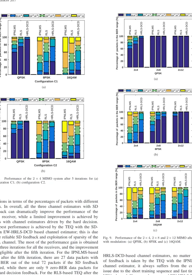
IPNLMS RLS HRLS-DCD IPNLMS RLS HRLS-DCD IPNLMS RLS HRLS-DCD QPSK 8PSK 16QAM Configuration C1 0 20 40 60 80 100
Percentage of packets in the BER range (%)
0 (0,10-4] (10-4,10-3] (10-3,10-2] (10-2,10-1] (10-1,1]
(a)
IPNLMS RLS HRLS-DCD IPNLMS RLS HRLS-DCD IPNLMS RLS HRLS-DCD
QPSK 8PSK 16QAM Configuration C2 0 20 40 60 80 100
Percentage of packets in the BER range (%)
0 (0,10-4] (10-4,10-3] (10-3,10-2] (10-2,10-1] (10-1,1]
(b)
Fig. 6. Performance of the2×4 MIMO system after 5 iterations for (a)
configuration C1; (b) configuration C2.
iterations in terms of the percentages of packets with different BERs. In overall, all the three channel estimators with SD feedback can dramatically improve the performance of the turbo receiver, while a limited improvement is achieved by TEQs with channel estimators driven by the hard decision. The best performance is achieved by the TEQ with the SD-driven EW-HRLS-DCD based channel estimator; this is due to the reliable SD feedback and exploitation of sparsity of the UWA channel. The most of the performance gain is obtained after three iterations for all the receivers, and the improvement is negligible after the fifth iteration. For the IPNLMS-based TEQ after the fifth iteration, there are 27 data packets with zero BER out of the total 72 packets if the SD feedback is used, while there are only 9 zero-BER data packets for the hard decision feedback. For the RLS-based TEQ after the fifth iteration, there are 54 zero-BER data packets for the SD feedback, while there are 38 zero-BER data packets for the hard decision feedback. For the EW-HRLS-DCD-based TEQ after the fifth iteration, there are 61 zero-BER data packets for SD the feedback, and only 40 zero-BER data packets for the hard decision feedback. As opposed to the RLS- and
IPNLMS RLS HRLS-DCD IPNLMS RLS HRLS-DCD IPNLMS RLS HRLS-DCD
2x4 2x8 2x12 QPSK 0 20 40 60 80 100
Percentage of packets in the BER range (%)
0 (0,10-4] (10-4,10-3] (10-3,10-2] (10-2,10-1] (10-1,1]
(a)
IPNLMS RLS HRLS-DCD IPNLMS RLS HRLS-DCD IPNLMS RLS HRLS-DCD
2x4 2x8 2x12 8PSK 0 20 40 60 80 100
Percentage of packets in the BER range (%)
0 (0,10-4] (10-4,10-3] (10-3,10-2] (10-2,10-1] (10-1,1]
(b)
IPNLMS RLS HRLS-DCD IPNLMS RLS HRLS-DCD IPNLMS RLS HRLS-DCD
2x4 2x8 2x12 16QAM 0 20 40 60 80 100
Percentage of packets in the BER range (%)
0 (0,10-4] (10-4,10-3] (10-3,10-2] (10-2,10-1] (10-1,1]
(c)
Fig. 9. Performance of the2×4,2×8and2×12MIMO after 5 iterations
with modulation: (a) QPSK, (b) 8PSK and (c) 16QAM.
HRLS-DCD-based channel estimators, no matter what kind of feedback is taken by the TEQ with the IPNLMS-based channel estimator, it always suffers from the convergence issue due to the short training sequence and fast time-varying UWA channel. However, the proposed EW-HRLS-DCD based channel estimator efficiently deals with this problem.
VII. CONCLUSION
In this paper, we have proposed and investigated a novel turbo equalizer for MIMO UWA systems with single-carrier