INFORMATIK
BERICHTE
366 – 10/2012
Simple and Efficient Coupling of Hadoop
With a Database Engine
Jiamin Lu, Ralf Hartmut Güting
Fakultät für Mathematik und Informatik
D-58084 Hagen
Simple and Efficient Coupling of Hadoop
With a Database Engine
Jiamin Lu, Ralf Hartmut G¨uting
Database Systems for New Applications, Mathematics and Computer Science FernUniversit¨at Hagen, Germany
{jiamin.lu,rhg}@fernuni-hagen.de
October 30, 2012
Abstract
The growing need of processing massive amounts of data leads database researchers to explore the possibility of combining their existing single-computer database systems with Hadoop. Such hybrid systems not only can keep the efficiency of database processing, but also achieve a remarkable scalability. However, current Hadoop extensions usually rely on Hadoop to shuffle intermediate data, in order to get a balanced workload assignment on cluster nodes. During the process, data in databases have to be transformed to key-value pairs and delivered to HDFS, hence can be processed in Hadoop jobs. These overheads cause a performance degradation of Hadoop hybrid systems.
In this paper, we propose a novel method to couple Hadoop and databases at the engine level rather than the SQL level, introducing query processing operators to interact with Hadoop. Distributed single-computer databases instead of Hadoop perform the task of shuffling intermediate data. Therefore, all data are exchanged between database engines directly, to reduce the unnecessary transform and transfer overhead. Query plans in the DBMS can be written to include the construction of Hadoop jobs, so that the user can write parallel queries in the DBMS without learning too many details of the MapReduce paradigm.
As a prototype of this method, Parallel SECONDO is demonstrated in this paper. It is fully evaluated with two parallel join methods, HDJ and SDJ, which respectively rely on Hadoop and SECONDO to shuffle data. The evaluation is not only made in our own small-scale cluster, but also in large-scale clusters consisting of hundreds of instances rented from the Amazon EC2 Cloud Service. In addition, Parallel SECONDOinherits the extensibility of SECONDO, it can also process specialized database queries on spatial and spatio-temporal data (or moving objects). As a result, we obtain for the first time a highly scalable generic system for moving objects management.
1
Introduction
For several years, the possibility to process massive amounts of data with the MapReduce ap-proach [8] has raised a lot of interest in database research. MapReduce offers the programmer a simple model of describing a highly parallel computation by just providing two kinds of simple functions manipulating sets of (key, value) pairs. The MapReduce execution system takes care of the rest, i.e., it creates tasks based on these functions for large sets of computers (nodes), distributes data between nodes, and supervises the execution of the tasks in such a way that failures of nodes or even slow executions do not seriously disturb or delay the execution of the
overall task. These fault-tolerance properties make MapReduce applications extremely scal-able and allow them to run on hundreds or thousands of nodes without problems. Hadoop [1] is available as an open source implementation of the MapReduce approach; hence it is open to anyone to organize large scale computations in this way.
Traditionally it was the job of highly optimized parallel database systems to process mas-sive amounts of data. While these systems show clearly better performance in basic data manip-ulation tasks, they were designed for clusters of limited size and do not have the fault-tolerance to deal with thousands of computers. Moreover, such systems require commercial licenses and are quite expensive.
Research has therefore tried to somehow move database functionality, e.g. performing joins or generally executing complex queries, into MapReduce or Hadoop executions. Some basic strategies for that are (i) to implement database operations as map or reduce functions, (ii) to extend the framework of MapReduce to make it better suited for database operations, e.g. to include a third type of function (merge) to process binary operations like joins, or (iii) to construct hybrid systems that take an existing database system and let it communicate with Hadoop. In this case Hadoop organizes query execution by giving tasks to instances of the DBMS distributed over many nodes. We call the participating DBMS a “single computer database system” (even though it is a client-server system capable to serve requests from many clients on other computers).
A motivation for the third approach is of course to reuse existing functionality in the DBMS. This motivation is increased if the single computer DBMS provides special capabilities that would be hard to reimplement from scratch in a MapReduce environment.
In this paper we also follow the third approach and we are in fact motivated by a
single-computer DBMS providing special functionality. The SECONDOsystem has unique
capabili-ties in the area of moving objects management (also calledtrajectory databases). It implements
a high level data model of moving objects [15, 12] providing a lot of advanced query
opera-tions. Moreover, SECONDOis constructed with a focus on extensibility, i.e., it is easy to add
even complex query processing operations. Combining SECONDOwith Hadoop should make
it possible to obtain a highly scalable moving objects DBMS, capable of handling massive tra-jectory databases, a problem that does arise in practice. In addition, this system would inherit
extensibility features from SECONDO.
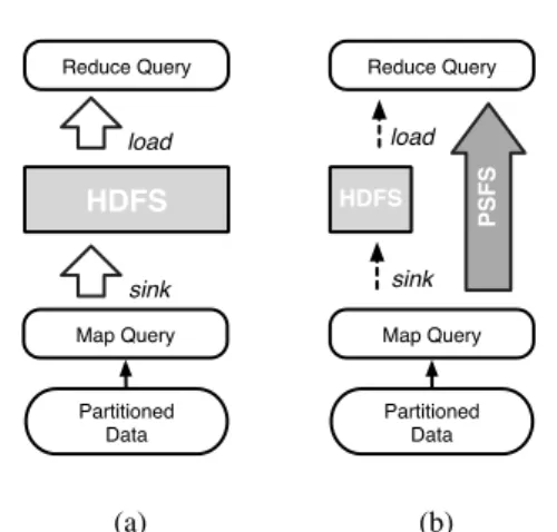
There exist several Hadoop hybrid extensions, combining Hadoop with existing single-computer databases, such as HadoopDB. However, these systems normally use the DBMS at the application level. The SQL-queries are embedded into MapReduce tasks, which are then processed by the single-computer databases. During this procedure, database data have to be exported into Hadoop’s distributed file system in the (key, value) format to achieve a balanced work-load assignment. Converting and transferring data between DBMS and Hadoop leads to some overhead, shown in Figure 1a.
Regarding the coupling of Hadoop with existing database systems, in this paper we propose a simple and efficient coupling method, in order to remove unnecessary overheads. We also make the hybrid-system compatible with the original way of using the DBMS. A prototype
Parallel SECONDOis demonstrated in this paper, which achieves the following targets:
1. Parallel SECONDOcouples our single-computer database system SECONDOwith Hadoop
on the engine level, introducing query processing operators to interact with Hadoop.
In-termediate data are exchanged between distributed single-computer SECONDOengines
directly, as shown in Figure 1b.
2. A parallel data model is provided in Parallel SECONDOto indicate distributed data over
Map Query Partitioned Data HDFS Reduce Query sink load (a) Map Query HDFS Reduce Query sink load Partitioned Data PSFS (b)
Figure 1: Data Flow in Hadoop-based Hybrid System
Thereby, the user can describe parallel queries in SECONDOexecutable language, as if
he/she is using a normal single-computer SECONDO.
3. The implementation of Hadoop is not affected, this approach can also be used to work with other Hadoop extensions, which improve the system on other aspects.
4. Besides, a set of auxiliary scripts is provided, in order to help the user set up and use
Parallel SECONDOas easily as possible.
5. As a result, a highly scalable and extensible moving objects DBMS becomes available.
Particularly, in this paper the join operation is used to present and evaluate Parallel SEC
-ONDO, as join is widely studied by many other researchers [23, 18, 3]. Two join methods HDJ
and SDJ are introduced, which rely on Hadoop and SECONDOto re-distribute intermediate
data in the system, respectively. Both methods can be used to process various data types, in-cluding specialized data types like spatial and moving objects. In addition, these methods are
fully evaluated on both small and large sized clusters, in order to prove that Parallel SECONDO
inherits not only the efficiency and extensibility from SECONDO, but also the scalability from
Hadoop.
The rest of this paper is organized as follows. Section 2 reviews all related work about this
study, and Section 3 briefly introduces the single-computer SECONDO. Afterwards, the
infras-tructure of Parallel SECONDOand the parallel data model is proposed in Section 4, together
with the two parallel join methods. Section 5 provides the evaluation of the system in different sized clusters. At last, we conclude with the future work of this study in Section 6.
2
Related Work
By virtue of its runtime scheduling scheme and high fault-tolerance performance, Hadoop can be easily deployed on large-scale clusters consisting of hundreds and even thousands of low-end computers. It attracts considerable attention from both academic and industry institutions. However, its efficiency is often questioned [23, 18]. Therefore, a lot of Hadoop extensions are proposed in recent years, which can be roughly divided into three kinds.
The first kind of Hadoop extensions attempts to improve the expressivity of Hadoop. A Hadoop user is forced to implement ad-hoc programs for different queries, as there is no declar-ative language provided in Hadoop. These custom pieces of user code are hard to maintain and
reuse, creating barriers for co-workers. Regarding this issue, the project Pig [21] provides a language named Pig Latin. It provides a nested data model and corresponding operators, allow-ing the user to describe queries as Pig Latin programs which can then be compiled to Hadoop jobs automatically. HiveQL proposed in the project Hive [25] is another Hadoop declarative language. It converts the user’s SQL-like queries to MapReduce jobs after the compilation. Specifically, Hive views the HDFS as a data warehouse and offers an external metastore to keep schemas of involved data, in order to optimize the generated jobs. SQL/MapReduce [13] introduces the MapReduce paradigm to parallel DBMSs, instead of providing SQL-like lan-guages to Hadoop. The user describes MapReduce jobs in SQL queries by fulfilling necessary clauses in SQL/MapReduce UDFs, which are executed as normal SQL sub-queries, in their underlying parallel database nCluster.
The second kind of Hadoop extensions enhances Hadoop on particular database operations. Hadoop emphasizes on keeping its scalability and fault-tolerance feature, hence it lacks a lot of technologies developed in the database community for decades. Particularly, the join has the largest performance difference between Hadoop and Parallel DBMSs [23]. In a Hadoop
job, the join operation happens on either the Map stage or the Reduce stage, and the latter
situation is more common. In this case, heterogeneous data sets must be homogenized into (key,
value) format, and then be redistributed by Hadoop in order to achieve a balanced workload assignment. Following this basic strategy, [4] proposes different algorithms and preprocessing methods for equi-join operations on vast amounts of log records. On the one hand, if there occur large size differences between two tables, records from the smaller table are either delivered to reducers ahead of the others in order to be fully buffered into memory, or are broadcast among the cluster without repartitioning the large table. On the other hand, when the join happens on two large tables, one table is filtered by aggregated join keys from the other table first before being joined, so as to reduce the communication overhead as much as possible. Besides strictly following the MapReduce paradigm, some other works propose MapReduce variants for the join operation by providing more flexible data flows. Map-Reduce-Merge [30] improves Hadoop on processing heterogeneous operations like the one-round join query. It adds an
extra predicateMerge to the programming model afterReduce, so as to avoid homogenizing
both inputs. Thereby, two heterogeneous relations can be processed independently and then be
joined at the lastMergestage. It also provides several configurable components, for the purpose
of controlling the progress of the operation and implementing different merge algorithms. The third kind of extensions addresses the runtime scheduling scheme in Hadoop, which
divides a Hadoop job into two blocked stagesMapandReduce, and no reduce task can start
when at least one map task is still running. Therefore, studies like MapReduce Online [6] attempt to build a pipeline between map and reduce tasks, while [27] proposes a new merge
algorithm in shuffling intermediate data betweenMapandReducestages.
More or less, the above Hadoop extensions need to invade the implementation of the Hadoop framework, and may affect its scalability. Therefore, hybrid systems of Hadoop and other existing database systems are proposed, in order to take the best features from both sides. HadoopDB [3] attempts to combine the Hadoop framework with single-node databases. It de-pends on Hive to compile SQL-style queries into Hadoop jobs, each task pushes the assigned sub-queries into slaves’ high-performing DBMSs which are more suitable for processing re-lational database operations, while Hadoop is only used as the task coordinator and the com-munication level. On the one hand, HadoopDB inspires our work in this paper, using Hadoop as the task coordinator and the communication level. On the other hand, we intend to cou-ple Hadoop with other database systems on the engine level by exchanging as few as possible data with HDFS. There are also other hybrid systems which use Hadoop to be their auxiliary components. The study in [28] shows the integration of Hadoop with parallel DBMS Teradata
EDW. It tightly and efficiently migrates data between these two systems, since many customers attempt to use both to process their business data. DEDUCE [19] combines Hadoop and Sys-tem S, since the latter is better suitable for real-time stream processing, but less efficient on analyzing large amounts of stored data. By extending an operator that is also named MapRe-duce, Hadoop jobs are embedded into its SPADE data-flow, and their results can be delivered to other operators as input.
Spatial and spatio-temporal data are not directly supported in Hadoop, since they are rep-resented and processed with specialized data models [12] and algorithms [20]. Therefore, there only exist studies on processing several particular spatial queries. SJMR [31] proposed a method for processing the parallel spatial join operation. Objects from both sides are divided into partitions evenly, and each partition is independent from the others. Therefore, objects can be distributed to slaves by partitions, and all slaves can process the join operation in par-allel. A similar idea is also adopted in this paper. BRACE [26] uses MapReduce to simulate agents’ behaviors in parallel. It abstracts behavioral simulations in the state-effect program-ming pattern, which can be processed as iterated parallel spatial join operations, with two con-secutive MapReduce jobs at each time. Several studies examine processing specialized data with other scalable frameworks instead of MapReduce. [5] specifically studies the grid-based map-matching procedure in parallel, which can be viewed as an application of the spatial join operation, with IBM’s System S.
3
Single-Computer Secondo
SECONDO is a DBMS prototype developed at University of Hagen. Two main goals in the
development are extensibility and the support of spatial and spatio-temporal applications. In particular, an advanced data model for the handling of moving objects (also called trajectories) as described in [16] has been implemented to a large extent.
The system consists of three major components: the kernel, the query optimizer, and the graphical user interface. The kernel represents the execution system of a DBMS. With regard
to extensibility, the SECONDOkernel does not assume a fixed data model (such as a relational
model, for example). Instead, the entire implementation of a data model is structured into algebra modules, each providing some data types and operations. Data types can be as simple
as an integer or a spatial typeline, or as complex as a relation or an index structure. Operations
can be multiplication of integers, a hashjoin on two tuple streams, or an exact match search on a B-tree. Operations can process arguments or yield results in pipelined mode, represented by
astreamtype in SECONDO. They can also have function arguments (e.g. a selection condition
would be a parameter function for an operator filtering a tuple stream).
The kernel is implemented on top of Berkeley-DB which as a storage layer takes care of transactions, recovery, etc. The kernel is essentially an engine that evaluates arbitrary expres-sions over operators of the available algebras, applied to database objects and constants. Such
expressions are at the same timequery plans.
A to our knowlegde unique feature of SECONDOis that query plans can be typed by the
user directly; they are type-checked by the system and then executed. We call this language level the executable language. A simple plan that could be typed by a user is
query Vehicles feed filter[.Type = "truck"] consume
corresponding to an SQL query
Operations in executable language are usually written in postfix notation in the order in which
they are applied. In the above query,feedis applied to a relation, delivering tuples in stream
mode,consumecollects a tuple stream into a relation which is then the result of the query.
In this paper, we make use of the kernel’s extensibility. Two algebras namedHadoopand
HadoopParallelare implemented. Each contains data types and operators that are designed to
combine SECONDOwith Hadoop. All operators in the HadoopParallel algebra can be used in
a single-computer SECONDOsystem as well, whereas the operators provided in the Hadoop
algebra can only be used in Parallel SECONDO, with the involvement of Hadoop. Their data
types and operators are presented in the next section. After providing these two algebras, the
user who has used single-computer SECONDOcan quickly get familiar with Parallel SECONDO
and use all old functions as usual.
The complete system provides querying at two language levels, namely SQL or executable
language. The SECONDOquery optimizer maps queries in an SQL-like language to plans in
the executable language, applying cost-based optimization. At present, parallel queries can be described only in the executable language. SQL-like parallel queries are not available yet, as the work of integrating this study into the query optimization is ongoing.
SECONDOalso provides a Client-Server structure, hence it has the ability of being remotely
accessed. Once a server process named SECONDO-Monitor starts, a number of SECONDO
client terminals can visit its database by indicating its IP address and port number. Each client
starts a SECONDOinstance on the server side. Depending on this feature, every cluster node can
run several SECONDOinstances during parallel procedures, in order to fully use the computing
resources of the cluster.
BerlinMOD [11] is a benchmark prepared for evaluating moving objects databases, with a simulated data set and common moving objects queries. The user can create and process different BerlinMOD data sets by simply setting a scale factor. When it is set to be 1, historic trajectories of 2000 vehicles running on the street network of Berlin in 28 days are simulated, requiring 11 GB of disk space. The queries enumerated in BerlinMOD are divided into two sets, 17 range and 9 nearest-neighbor queries. Generating the data and processing them with the queries in BerlinMOD are expensive. For example, the creation time for the data set with the scale factor of 1 takes about 15 hours, while processing it with all 17 range queries takes
an-other 20 hours. Regarding this issue, Parallel SECONDOalso helps to enhance BerlinMOD on
simulating large data sets and processing several particularly expensive queries. More details are introduced in Section 4 and Section 5.3.
4
Parallel Secondo System
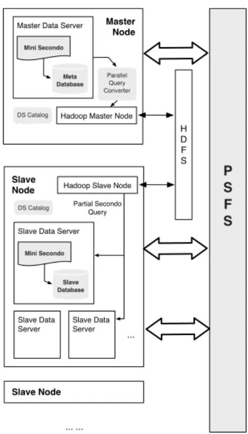
Parallel SECONDOis constructed by coupling Hadoop with a set of single-computer SECONDO
systems, as shown in Figure 2. In principle, the two components work independently. Hadoop is used as a kind of “distributed operating system”, applying and scheduling tasks to slaves. The
tasks are then processed in single-computer SECONDOdatabases. Hadoop is used transparently
to end-users, who use Parallel SECONDOlike a standard single-computer SECONDO.
Parallel SECONDOis set up based on data servers (DS) instead of nodes. In Hadoop, each
cluster node is viewed as a worker. A particular node is set as the master, while the others are all set as slaves. Nodes in Hadoop communicate with each other through the HDFS (Hadoop Distributed File System). Nowadays, it is common that a low-end PC may have one or more processors with multiple cores, several hard disks and a large amount of memory. Therefore,
in order to fully use the capability of the underlying cluster, we set adata server(DS) as the
minimum execution unit in Parallel SECONDO. A DS holds several cores, part of the disk
Slave Node
Master Node
Hadoop Master Node Master Data Server
Mini Secondo Meta Database DS Catalog Parallel Query Converter Slave
Node Hadoop Slave Node
Slave Data Server Mini Secondo
Slave Database
DS Catalog Partial Secondo
Query ... ... P S F S H D F S Slave Data Server Slave Data Server ...
Figure 2: Framework of Parallel Secondo
data exchanged among DS are transferred through the PSFS (Parallel Secondo File System),
which is a simple distributed file system prepared for Parallel SECONDOthat will be introduced
below. The infrastructure of Parallel SECONDOis shown in Figure 2. Each DS contains a
compact SECONDOnamed Mini-SECONDO, its database storage and a PSFS node. With an
auxiliary script, all Mini-SECONDO instances are built based on a normal single-computer
SECONDO system. Therefore, in case any changes or extensions to algebras are applied in
SECONDO, it is easy for the user to update all Mini-SECONDOinstances rapidly.
PSFS (Parallel Secondo File System) is built as a substitute of HDFS, being used to
ex-change data between Mini-SECONDOdatabases directly without passing through HDFS. Data
kept in PSFS nodes are delivered with the pull model, as in the HDFS used in Hadoop. Re-garding the issue of fault-tolerance, the chained-declustering mechanism [29] is used in PSFS; each data piece can be duplicated to several DS to provide for problems arising at run-time. In order to indicate the locations of DS, a DS-Catalog is made up and duplicated on every cluster
node. The DS-Catalog usually is set up by the user when installing Parallel SECONDO. All
operators that have been added in Parallel SECONDOfor accessing data in PSFS are named
PSFS operators, which will be further introduced in Section 4.4.
In Parallel SECONDO, one and only one particular data server is set to be the master DS,
which is the sole entrance for the user, keeping all global and meta data of the whole system. It
is possible for the user to set his existing SECONDOdatabase to be the database storage in the
master DS, to enable the user to use Parallel SECONDO directly without migrating any data.
In this way, the user can easily choose either single-computer or Parallel SECONDOto process
4.1 Example Parallel Query
In order to introduce Parallel SECONDO clearly, an example query is demonstrated here to
display the process of converting a sequential query into the corresponding parallel query. The example is the 6th range query from the BerlinMOD benchmark which requires to find in a set of vehicle trajectories all pairs of trucks that have been as close as 10 meters or less to each other, sometimes within the observation period. This query will also be evaluated experimentally in the next section.
Note that the trajectory of a vehicle is a curve in the three-dimensional(x, y, t)space [12].
Hence the problem is essentially to perform a spatial join in the 3D space, finding pairs of pieces of the curves that are close to each other. This can be solved by enlarging bounding boxes of
such pieces by the distance in(x, y)and then to find pairs of overlapping three-dimensional
boxes.
A state-of-the-art spatial join method is PBSM (partition based spatial merge join) [22, 31] which can easily be parallelized. Basically, a 3D grid is defined and the pieces of the trajectories
(calledunits) of both arguments are distributed over the grid, i.e. entered into any grid cell they
intersect. Grid cells are then grouped into partitions, e.g. by an assignmentp := c mod k,
wherep is the partition index, c the cell index, and kthe number of partitions. The goal is
to distribute densely and scarcely populated cells evenly to partitions so that all partitions get roughly the same number of entries. Further, a partition should fit into memory. Next, PBSM sequentially loads each partition into memory and processes the join by some method such as plane sweep. Care has to be taken to avoid duplicate reports, i.e. the same two objects “meeting” in two different cells. Obviously, partitions can be handled in parallel as well.
A simple method to process the join within each partition is to sort and group the two sets of partition entries by cell numbers and then to perform the join within each cell by evaluating all pairs. We use this method for the following example.
This method can be expressed as a query, both in standard and parallel SECONDO, after
extending SECONDO by a few auxiliary query operators called cellnumber, gridintersects,
and parajoin2. Operator cellnumber takes a definition of a regular grid in 2D or 3D and
returns for a given rectangle r the set of cell numbers of cells intersected by r. Operator
gridintersectstakes a definition of a grid, two rectanglesrands, and a cell numberc; it returns
trueif the two rectangles intersect and the (unique) smallest point of their intersection lies in
cellc. This ensures that duplicate reports from different cells are avoided, a technique from
[10]. Finally,parajoin2is similar to mergejoin in taking two sorted input streams. Whereas
mergejoin returns for each pair of groups of tuples with the same attribute value the Cartesian
product,parajoin2allows one to apply a generic parameter function to process these groups of
tuples. Hence one can apply any desired join method to two such groups. Operatorparajoin2
is motivated by a similar operatorparajoindesigned for use with Hadoop and explained below.
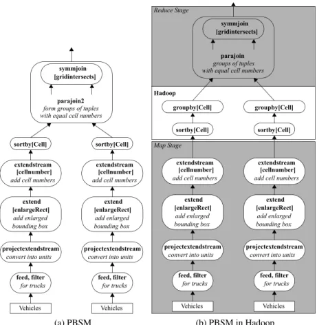
The sequential SECONDO query implementing PBSM is presented in Figure 3a. The
V ehicles relation is fed into a stream of tuples and filtered to select trucks. In the next
op-erator (projectextendstream) for each tuple the trajectory is converted into a set of units and
removed from the tuple; instead, for each unit a copy of the rest tuple with the unit appended is returned. Hence at this point instead of a stream of (tuples with) trajectories we have a stream of tuples with units. In the next step, the enlarged bounding box of the unit is appended to each tuple. Then the cell numbers are computed and appended, copying the tuple if needed (i.e., more than one cell number). Streams are then sorted by cell numbers and with the help
ofparajoin2for each pair of cells the join is computed based on thegridintersectstest.
As-suming that the number of entries per cell is small, a symmetric variant of the nested loop join
Vehicles feed, filter
for trucks
projectextendstream
convert into units
extend add enlarged bounding box extendstream [enlargeRect] [cellnumber]
add cell numbers
sortby[Cell]
Vehicles feed, filter
for trucks
projectextendstream
convert into units
extend add enlarged bounding box extendstream [enlargeRect] [cellnumber]
add cell numbers
sortby[Cell] symmjoin
[gridintersects]
parajoin2
form groups of tuples with equal cell numbers
(a) PBSM
Vehicles
feed, filter for trucks projectextendstream
convert into units extend add enlarged bounding box extendstream [enlargeRect] [cellnumber] add cell numbers groupby[Cell]
Vehicles
feed, filter for trucks projectextendstream
convert into units extend add enlarged bounding box extendstream [enlargeRect] [cellnumber] add cell numbers groupby[Cell] symmjoin
[gridintersects]
parajoin groups of tuples with equal cell numbers
Map Stage Hadoop Reduce Stage
sortby[Cell] sortby[Cell]
(b) PBSM in Hadoop
Figure 3: Data Flow of Sequential and Parallel Spatial Join
SECONDO. The precise sequential query is shown in the Appendix in Table 10.
4.2 Parallel Data Model
The workflow of the example sequential query can be easily divided into 2 stages, following the
MapReduce paradigm, as shown in Figure 3b. In theMapstage, all units are partitioned into
the cell grid. Afterwards, thesymmjoinandgridintersectsoperations can be performed
by all data servers independently in theReduce stage. Beyond that, Hadoop takes charge of
sorting and shuffling units based on their cell numbers.
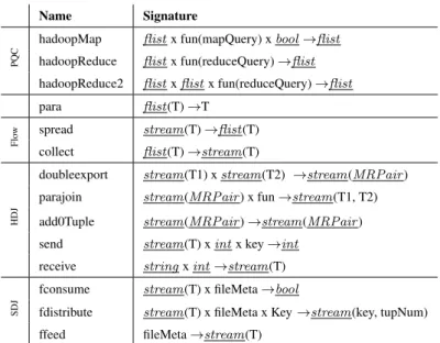
In order to describe this parallel query in Parallel SECONDO and convert the query into
Hadoop jobs, a parallel data model is studied, a data type and a set of operators are then
provided as extensions in the newHadoopalgebra. Table 1 shows operators provided as
ex-tensions for Parallel SECONDO. They are explained in the following discussion.
In the approach presented, we will execute the same queries on many data servers. A question is what an object name refers to in a query, that is, is it the same object on all data servers or is it a distinct part of an object to be handled just by this data server. Therefore, we
classify Parallel SECONDOdatabase objects according to their size and whether they are equal
or different on different data servers, as shown in Table 2. Small sized objects like an integer or instant take only a few bytes, whereas large objects like a relation can be as large as hundreds
of gigabytes. At the same time, the value of an objectomentioned in a query may be equal
or vary on different data servers. For example, the cell grid data structure used in the example query is very small, being described with several real numbers, and being identical on every
Name Signature
PQC
hadoopMap flistx fun(mapQuery) xbool→flist hadoopReduce flistx fun(reduceQuery)→flist hadoopReduce2 flistxflistx fun(reduceQuery)→flist
para flist(T)→T
Flo
w spread stream(T)→flist(T)
collect flist(T)→stream(T)
doubleexport stream(T1) xstream(T2) →stream(MRPair) parajoin stream(MRPair) x fun→stream(T1, T2) HDJ add0Tuple stream(MRPair)→stream(MRPair)
send stream(T) xintx key→int
receive stringxint→stream(T)
fconsume stream(T) x fileMeta→bool
SDJ fdistribute stream(T) x fileMeta x Key→stream(key, tupNum)
ffeed fileMeta→stream(T)
Table 1: Operators Provided as Extensions In Parallel SECONDO
Small Size Large Size
Equal DELIVERABLE Duplicated
Varying PS-Matrix PS-Matrix
Table 2: The Classification of Partitioned Objects
data server. Therefore, it is a small and equal object. In contrast, the relationVehiclesis large,
since it contains hundreds of vehicles’ trajectories over days, and each data server should work on a distinct subset of it. Hence it is a large and varying object.
Based on this classification, objects are treated differently. Small and equal objects, like the cell grid, are created and saved only in the master database. When required, their values are broadcast to every involved data server along with the query. Keeping and updating these ob-jects is the same as in single-computer databases. This kind of data is called DELIVERABLE data, since their values are delivered during the run time.
Varying objects oare partitioned as PS-Matrices with two distribution functions, named
Row(o)andColumn(o), as shown in Figure 4. Theocan be all kinds of SECONDOobjects,
like a relation or an index structure. TheRow(o)divides the data intoR parts, each part can
only be kept on one data server and hence be viewed as one row in the PS-Matrix. It is possible
for Row(o) to produce more rows than the cluster scaleN, and let one data server contain
multiple rows. Afterwards, Column(o) further divides rows to C columns, and creates an
R×C PS-Matrix at last. It is possible that few pieces of the PS-Matrix have no data at all,
because of the skewed distribution of the data set, like the white blocks shown in Fig 4. Besides
the above three situations, large and equal objects may also exist in Parallel SECONDO, which
means full replication.
Parallel SECONDOespecially introduces a type constructorflist to describe PS-Matrices.
It is designed as a wrap structure, in order to encapsulate all available SECONDOtypes. Hence
for any typeαthere is a corresponding typeflist(α). For example, for typepointthere is a type
flist(point) and forrel(tuple(X)) there existsflist(rel(tuple(X)). After a SECONDOobject has
been distributed into a PS-Matrix, pieces of data are kept in slave data servers; only their entry
Data Server 1 Data Server N Data Server 2 Data Server 1 Data Server m ... ... ... ... ... ... ... ... ... ... ... ... ... ... C R N Figure 4: PS-Matrix
There are two methods of keeping piece data in PS-Matrices on slave data servers. The first
stores the data in slave Mini-SECONDOdatabases as normal SECONDOobjects. The second
exports data to PSFS as disk files. Hereby, there are two kinds of flist objects in Parallel
SECONDO.
1. Distributed Local Objects (DLO): A DLOflist object divides a large-sized SECONDO
object to aN ×1PS-Matrix, each piece is kept in one and only one Mini-SECONDO
database, as a normal SECONDOobject, called sub-object. All sub-objects of a same flist
share the same name in slave databases. DLOflistcan wrap all available SECONDOdata
types.
2. Distributed Local Files (DLF): Data are divided into aR×CPS-Matrix, and each piece
is exported as a disk file, saved in several PSFS nodes, called sub-files. TheRandCare
determined by their distribution functions. Sub-files are processed by PSFS operators, and they can be transferred among data servers during parallel procedures. At present,
DLFflistis prepared for relations only, since the other types data cannot be exported as
sub-files.
Operatorsspread andcollect(Table 1, Section Flow) are available to concatenate
se-quential and parallel queries. Herespreadpartitions a tuple stream into the cluster and
re-turns anflistobject. In contrast,collectgathers all data in anflist object from the cluster and
returns them in a stream of tuples.
Besides representing partitioned objects, three PQC (Parallel Query Converter) operators
(Table 1, Section PQC) are provided in Parallel SECONDO, to describe parallel queries in
SECONDOexecutable language. Each operator contains a template Hadoop job, which creates
job instances according to input arguments. A function parameter is needed in every PQC operator, describing a sequential query that will be performed in one stage of the created job instance.
The function in both hadoopMap andhadoopReduce supports a unary query.
As-sume the inputflistobject is anR×CPS-Matrix, then in thehadoopMapoperation,Rmap
tasks start in the job instance and each processes one row of data of the input PS-Matrix. If
such anflistobject is processed by ahadoopReduceoperator,Creduce tasks start in the job
provides a binary query. Assume the two inputflist objects describeR×CandR0 ×C0
PS-Matrices respectively, andR0 ≥R. Accordingly,R0map tasks start and each processes at least
one row of data from each input PS-Matrix, then distributes the result intoK columns based
on a new distribution function. The map result builds up two intermediateR×KandR0×K
PS-Matrices. At last,K reduce tasks start and each processes one column of data from each
intermediate PS-Matrices with the indicated function. In each map or reduce task, the function
argument is converted into a sequential query, and processed in Mini-SECONDOdatabases, in
order to achieve a high efficiency.
The three presented PQC operators allow one only to specify one stage of a hadoop job, i.e., either a map stage or a reduce stage. As described, it would be necessary to create separate Hadoop jobs for the map and the reduce stage. Of course, it is preferable to have only one Hadoop job for both stages.
In principle it would be desirable to introduce a hadoop operator with two parameter
functions (queries), one for the map stage and one for the reduce stage. Unfortunately, this
is currently not possible with the SECONDOquery processor which performs complete type
checking of queries. For two parameter functions, the result type of the first query would need to be transfered into the type checking of the second query which is currently not available. However, there is a simple way to circumvent this problem.
To solve it, thehadoopMaptakes an additional boolean parameter, called executed. If
executed is set as f alse, the operator does not start up the Hadoop job but only returns an
flist containing the unexecuted function argument. This flist can then be delivered to the
hadoopReduceorhadoopReduce2operator, and execute the unexecuted function there
in the Map stage. Thereby it is possible to write a Parallel SECONDO query which starts a
Hadoop job with both stages containing map and reduce queries.
It happens that the query function accepted by a PQC operator also uses other partitioned data. In this case, on the one hand, all DELIVERABLE objects can be represented in the nor-mal way, as they can be detected by PQC operators automatically and their values be embedded into the function directly. On the other hand, if these data are distributed in the cluster and
rep-resented as anflistobject, an auxiliary operator calledparais used to access these objects. It
makes the object wrapped inflistagain available under the original data type.
4.3 HDJ Hadoop Distribute Join
Traditionally, Hadoop extensions rely on HDFS to distribute intermediate data, in order to
achieve a balanced workload on nodes. All data shuffled in HDFS must follow the (key, value)
format. In queries involving several data sets, heterogeneous data have to be homogenized before being shuffled in HDFS. For example, by using Hadoop to process a join with two
relationsR andS, each tuple from either side extracts its join attribute value as thekey, and
sets thevalue as a pair (tv, tag) in the map stage. The tv is the tuple value, while the tag
indicates which side this tuple comes from. Afterwards, homogenized (key, value) pairs are
shuffled in HDFS, and pairs with samekey are aggregated into a same reduce task. In each
reduce task, tuples are distinguished into two parts again based on thetagand restored from
tv, then the join can be executed at last. This join method is widely studied and evaluated
in [23, 3, 4]. Therefore, it is also implemented in Parallel SECONDO, named HDJ (Hadoop
Distribute Join), to be compared with our novel method that will be introduced later. A set of
operators are provided as extensions in Parallel SECONDOfor HDJ, listed in Table 1, Section
HDJ.
The general work flow of HDJ is shown in Figure 5. Next we explain it for the example query.
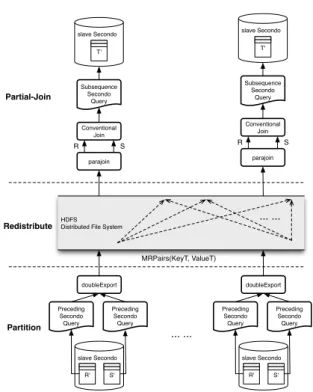
doubleExport Preceding Secondo Query Preceding Secondo Query slave Secondo R' S' doubleExport Preceding Secondo Query Preceding Secondo Query slave Secondo R' S' ... ... HDFS Distributed File System
MRPairs(KeyT, ValueT) ... ... parajoin Conventional Join R S Subsequence Secondo Query slave Secondo T' parajoin Conventional Join R S Subsequence Secondo Query slave Secondo T' Partition Redistribute Partial-Join
Figure 5: Hadoop Distribute Join
The HDJ work flow of the example query is shown in Figure 6a. The relation Vehicles
is first distributed into the cluster with the spread operation. Then it is processed by a
hadoopMapoperator to distribute trajectory units into the cell grid. Here the function ar-gument is the map query shown in Figure 3b. Afterwards, tuples containing units from both
sides are homogenized to HDFS with the operatordoubleexport. The intermediate data
type shuffled in HDFS is named MRPair, each contains one unit tuple, having two attributes:
KeyT andValueT. TheKeyT is the cell number of the unit, while theValueT contains the unit
tuple’s binary data and atagindicating its source relation. At the end of the map stage,
MR-Pairs are exported from distributed Mini-SECONDOdatabases to HDFS by using the operator
send, which works together withreceiveto transfer tuples through a TCP/IP channel. Later
Hadoop shuffles and aggregates MRPairs with the identicalKeyT value, i.e. the cell number,
into the same reduce task. In each reduce task, a distributed Mini-SECONDOimports the
as-signed MRPairs into a query tuple stream with the receiveoperator. Afterwards, MRPairs
are restored to unit tuples with the operatorparajoinand distinguished to two sides based on
theirtagvalues. At last, the reduce query shown in Figure 3b computes the join within cells.
In order to let the data be redistributed evenly and achieve a balanced workload on slaves, the cell grid is fine-grained. Therefore, the number of cells is far larger than the number of reduce tasks, and each reduce task needs to process a number of cells. In order to distinguish
MRPairs belonging to different cells, a special MRPair called 0Tuple is proposed. Thetagin
0Tuple is set to be 0, indicating it belongs to no side. 0Tuples are inserted between cells of
MRPairs, when Hadoop sends MRPairs ordered by cell numbers to Mini-SECONDOinstances.
Theparajoinoperator receiving such a stream of homogenized tuples and decoding it into two
separate streams views 0Tuples as separators between groups.
In order to be able to test the sequencedoubleexport-parajoinalso in a sequential SEC
-ONDO system, there is a further auxiliary operator add0Tuplewhich inserts 0Tuples into an
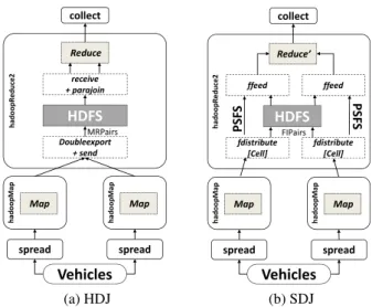
spread hadoopMap Map Doubleexport +send hadoopR e duce2 HDFS receive +parajoin Reduce collect hadoopMap Map MRPairs spread Vehicles (a) HDJ PSF S PSF S fdistribute [Cell] hadoopR e duce2 HDFS ffeed Reduce’ collect fdistribute [Cell] ffeed hadoopMap Map hadoopMap Map FIPairs spread spread Vehicles (b) SDJ
Figure 6: PBSM in Parallel Secondo
Theexecutedargument in thehadoopMapoperation is set to bef alse, hence the HDJ is
processed with one Hadoop job created in thehadoopReduce2operation. Besides, all
op-erators provided as extensions for HDJ are encapsulated inside the Hadoop job, being invisible for the user. Therefore, the user can set their query function parameters directly based on the sequential query.
4.4 SDJ Secondo Distribute Join
In HDJ, two kinds of overhead are produced. The first is the transforming cost between tu-ples and MRPairs, since every unit tuple has to be encapsulated into an MRPair in the map
stage, and extracted later in reduce tasks. The second is the transferring cost between SEC
-ONDOdatabase system and HDFS, as MRPairs have to be delivered twice between HDFS and
Mini-SECONDOdatabases. Such overheads are unavoidable if the system relies on HDFS to
redistribute intermediate data, causing performance degradation.
In this paper we propose a new method, which transfers intermediate data via PSFS instead
of HDFS. In this way, data can be delivered between SECONDOdatabases directly, and both
above overheads can be removed. This method is named SDJ (SECONDO Distribute Join),
since it mainly relies on Mini-SECONDOto redistribute data between map and reduce stages.
The general work flow of SDJ is shown in Figure 7.
All operators provided as extensions for SDJ are listed in Table 1, Section SDJ. These
operators are also called PSFS operators, since they are used to exchange data between PSFS
and SECONDOdatabases. Bothfconsumeandfdistributeexport relations (tuple streams
in queries) to PSFS as files, and ffeed reads files back into a SECONDO query. A relation
(or other object) in PSFS is represented in two kinds of files, namelytype filesanddata files.
The type file describes the schema of the exported relation, while the data file contains tuples’ binary block data. Keeping the small type file separately from the large data file allows one to first verify the correctness of the query expression without copying the large data file.
Operator fconsume exports the data to one data file, while fdistribute partitions the
data to several data files based on a specificKeyattribute. All PSFS operators can access data
not only on the local PSFS node, but also on remote computers in the cluster. Information
about positioning files in PSFS are indicated byfileMetaparameters.
... ... fdistribute Preceding Secondo Query Preceding Secondo Query slave Secondo R' S' fdistribute
Local File System
. . . . . . fdistribute Preceding Secondo Query Preceding Secondo Query slave Secondo R' S' fdistribute
Local File System
. . . . . . ffeed Conventional Join Subsequence Secondo Query slave Secondo T' ffeed ffeed Conventional Join Subsequence Secondo Query slave Secondo T' ffeed HDFS Distributed File System
..
Partition Redistribute
Partial-Join
FIPairs(KeyT, ValueT)
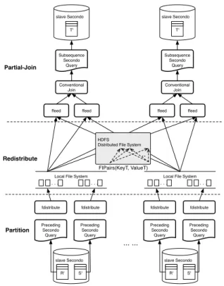
Figure 7: Secondo Distribute Join
database data are exchanged via PSFS, while their meta information are shuffled by Hadoop, in order to evenly assign the workload on data servers. The meta information is represented
by FIPairs (File Information Pair), which are also created according to the (key, value) format
in Hadoop. As we said in the above introduction for PQC operators, two intermediate
PS-Matrices are produced after the Map stage. Each FIPair describes one piece of data in the
PS-Matrices, and itskeyis the data piece’s column number. Therefore, reduce tasks process
the map result by columns, and each task first uses the ffeedto collect data from PSFS by
copying all required files from all other nodes in the cluster.
In SDJ, both the unnecessary transforming and transferring cost in HDJ are removed, as
data are exchanged between Mini-SECONDOinstances directly via PSFS. Only few small-sized
FIPairs are shuffled in Hadoop, so as to assign tasks to reduce tasks. In the implementation, the
hadoopReduce2operator provides both HDJ and SDJ methods, distinguished by a boolean
flag. Therefore, SDJ can also be described withhadoopMapandhadoopReduce2
oper-ators, in the same way as HDJ. Theexecutedarguments in bothhadoopMapoperations are
set to befalse, hence the query can be finished with one Hadoop job. It is also the same that all
operators provided as extensions for SDJ are set inside the template Hadoop jobs, in order to
keep Parallel SECONDOtransparent for the user.
5
Evaluation
In this section, Parallel SECONDO is fully evaluated with the join operation based on three
different data types, including standard, spatial and spatio-temporal types. The evaluations are made not only in our small-scale cluster, but also in large clusters composed by rented virtual computers from the Amazon EC2 service.
Phenom(tm) II X6 1055T processor with six cores, 8 GB memory and two 500 GB hard disks, and uses Ubuntu 10.04.2-LTS-Desktop-64 bit as the operating system. A Hadoop 0.20.2 frame-work is deployed on the cluster, taking one computer as the master node. Since there are two hard disks on every computer, each computer sets two data servers, one on each hard disk;
the master DS is also used as a slave DS. Hence in total, this parallel SECONDOtestbed has 6
machines, 6 processors, 36 cores, 48 GB memory, 12 disks and 12 slave data servers. Data sets used for the evaluations are either generated by public benchmarks, or are provided by public organizations.
• The first data set is used for the standard equi-join operation, and is generated by
bench-mark TPC-H [7], which contains a suite of business oriented data. The benchbench-mark offers a generator to produce the data set, and can change the set size by using different scale factors. The benchmark also offers many queries to evaluate different database methods, from which we choose the 12th query to evaluate our methods in this paper. When the scale factor is 1, the two relations used by the 12th query, LINEITEM and ORDERS, have 6,001,215 and 1,500,000 tuples respectively, and take about 1.3 GB disk space all together.
• The second data set is used for the spatial join operation, using data from the
Open-StreetMap project [17], which describes the road network of the federal state North
Rhine-Westphalia in Germany. We convert the data set into a SECONDOrelation, named
ROADS, and use this relation to perform a spatial self-join operation with our methods. ROADS has 732,054 tuples, and takes 927 MB disk space. Each tuple contains one road that is represented with a polyline [12] and some other descriptive information, like the road’s name, type, length etc. In the following experiments, we need to execute queries with large data sets, but the size of ROADS is limited. Hence we enlarge the data set by duplicating it, and use duplication numbers as scale factors. At the same time, the duplicated roads are translated in space to not overlap the original data set, in order to avoid producing explosive join results along with the duplication.
• The last data set is generated by benchmark BerlinMOD [11], which has been introduced
before. The example query explained in the previous section is used to evaluate the system here.
The coefficients speed-up and scale-up [9] are often used to evaluate various parallel sys-tems and methods, hence they are also used in this paper. There are slightly different interpre-tations of speed-up in the literature, namely ratio of time required on small system over time required on large system [9] or ratio of time for sequential query over time for parallel query [14]. We use the latter interpretation in cases when we are able to compare a query running
sequentially in standard SECONDO with the parallel version. To make it clear we also call it
Parallel Improvement(PI).
5.1 Equi-Join On Standard Data
The 12th query in TPC-H is used to evaluate both HDJ and SDJ methods on standard data. It counts the times of delayed deliveries caused by choosing cheaper shipping. The time condition on the receipt date is removed from the query, to increase the query cost and make this query suitable to evaluate parallel systems.
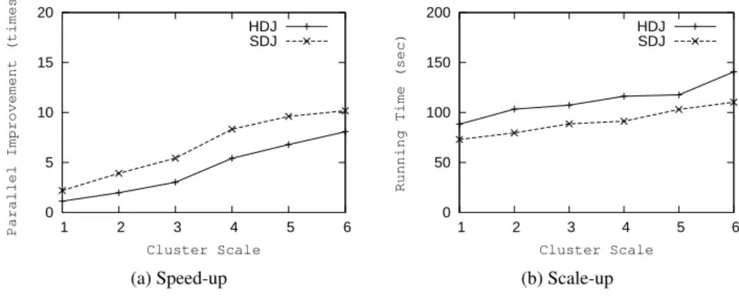
The evaluation of both methods is shown in Figure 8 and the respective queries are shown in Tables 3 through 5 of the Appendix. The scale of the cluster increases from 1 to 6. In the
0 5 10 15 20 1 2 3 4 5 6
Parallel Improvement (times)
Cluster Scale HDJ SDJ (a) Speed-up 0 50 100 150 200 1 2 3 4 5 6
Running Time (sec)
Cluster Scale HDJ SDJ
(b) Scale-up
Figure 8: Evaluation On Standard Data
speed-up evaluation, a constant-sized TPC-H data set with the scale-factor of 5 is used. It is clear that both methods keep a linear speed-up, and SDJ always shows a better performance than HDJ. The evaluation on scale-up is shown in Figure 8b. Here the scale factor of the data set also increases from 1 to 6. The result shows both methods keep a considerable stable scale-up by using more computers, and SDJ always shows a better performance than HDJ. The elapsed time of both increases slowly, when larger data sets are processed. This is mainly caused by the increasing transfer overhead along with the increase of data sets, since the network resource is shared by all slaves; it does not grow no matter how many slaves are used.
5.2 Spatial And Spatio-Temporal Join
The spatial join finds all pairs of intersecting roads in the relation ROADS, and the spatio-temporal join is the example query that we demonstrated in the last section. Both queries use the PBSM method, each uses a 2D and 3D cell-grid to partition the multi-dimensional data, respectively.
In the example query, we introduced a simple technique to perform the spatial join within a partition, namely to group the partition by cells and for each cell to evaluate all pairs. In this section we also evaluate a second method for performing the spatial join within a partition. This method uses a main-memory R-tree implementation (MMR-Tree). Here all tuples from
one data setRof the partition are read into memory and indexed in the MMR-Tree. Then all
tuples from the other data setSare scanned; for each of them the MMR-Tree onRis searched
to find matching tuples. So this is basically an index nested loop, building the index in memory on the fly.
In the experiments, we call the first method HDJ and SDJ and denote the MMR-Tree based method as HDJ’ and SDJ’. We compare HDJ with SDJ and SDJ with SDJ’.
Besides happening in 2D and 3D space, another important difference between the spatial and spatio-temporal join experiments is that the spatial join includes a refinement step, evaluat-ing intersections on the complete polyline data. This involves large object management leadevaluat-ing to special problems explained below.
At present, the scale of the cell-grids and cell sizes are determined before the queries start, by scanning the complete data sets. In the spatial join, streets are represented as polylines and partitioned into the 2D cell-grid. When a line covers several cells, the complete polyline is
duplicated into every passed cell, since it is needed in theReducestage for the refinement of
the spatial join. In the spatio-temporal join, as analyzed in Section 4.1, each trajectory’s units instead of complete trajectories are partitioned into the 3D cell-grid.
0 5 10 15 20 1 2 3 4 5 6
Parallel Improvement (times)
Cluster Scale HDJ SDJ (a) Speed-up 0 200 400 600 800 1000 1200 1400 1600 1 2 3 4 5 6
Running Time (sec)
Cluster Scale HDJ SDJ
(b) Scale-up
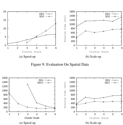
Figure 9: Evaluation On Spatial Data
0 200 400 600 800 1000 1200 1400 1600 1 2 3 4 5 6
Running Time (sec)
Cluster Scale SDJ SDJ’ (a) Speed-up 0 200 400 600 800 1000 1200 1400 1600 1 2 3 4 5 6
Running Time (sec)
Cluster Scale SDJ SDJ’
(b) Scale-up
Figure 10: Evaluation With Internal Index On Spatial Data
The performance of the spatial join is shown in Figure 9 and Figure 10 and the respective queries are given in Tables 6 through 9 of the Appendix. In the evaluation of the speed-up, the cluster increases from 1 to 6 nodes, while the scale factor of the data set is 2. Along with the increase of the cluster, more reduce tasks run in parallel and each task processes less data, hence the PI of both methods increase linearly. At first, SDJ performs worse than HDJ. Especially when there are less than 3 nodes in the cluster, SDJ even cannot finish the query.
The reason for this failure of SDJ on clusters of size 1 and 2 is on an abstract level simply that the resulting partitions are too big. Remember that PBSM tries to partition data so that each partition fits into memory. At a detailed level, the explanation is fairly involved and has
to do with the interaction of large object management and sorting in the SDJ query.1 However,
when the cluster scale is larger than 3, SDJ performs much better than HDJ, as we observed in the evaluation on standard data.
Additionally, the same speed-up evaluation is also made between SDJ and SDJ’, shown in Figure 10a. Here we compare the running times of SDJ and SDJ’ rather than the PI. With the
1
Theffeedoperator reads tuples from a file. Tuples from the ROADS relation contain polyline spatial data which are represented in so-called FLOBs (faked large objects). On reconstructing the tuple in memory, the large object part is put into a cache controlled by the FLOB manager. At the same time, due to the followingsortoperator which is blocking, no tuples can be released. For the large data sets considered, after a while the FLOB cache spills to disk; at the same time there are several memory-using operators which also spill to disk. Further, every data server has three cores but only one disk and the three reduce tasks interfere with each other on their disk accesses. This pulls down the performance of SDJ in such a way that for one or two nodes the running times get extremely high.
0 10 20 30 40 50 60 70 1 2 3 4 5 6
Parallel Improvement (times)
Cluster Scale HDJ SDJ (a) Speed-up 0 200 400 600 800 1000 1200 1400 1600 1 2 3 4 5 6
Running Time (sec)
Cluster Scale HDJ SDJ
(b) Scale-up
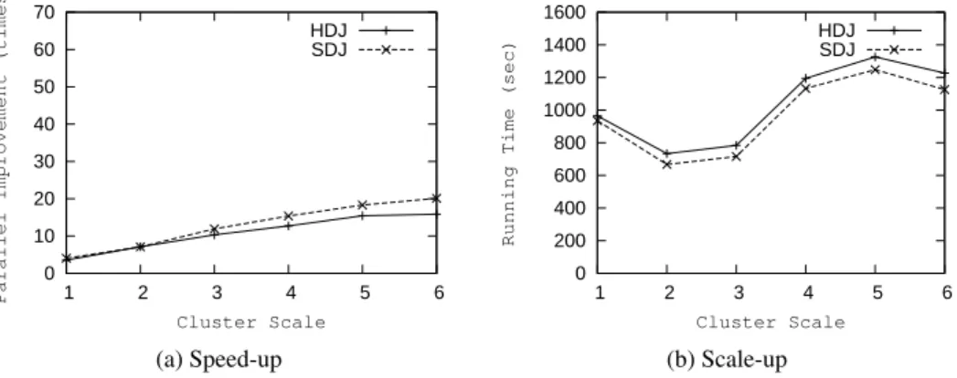
Figure 11: Evaluation On Spatio-temporal Data
0 200 400 600 800 1000 1200 1400 1600 1 2 3 4 5 6
Running Time (sec)
Cluster Scale SDJ SDJ’ (a) Speed-up 0 200 400 600 800 1000 1200 1400 1600 1 2 3 4 5 6
Running Time (sec)
Cluster Scale SDJ SDJ’
(b) Scale-up
Figure 12: Evaluation With Internal Index On Spatio-temporal Data
help of the index-based join operation, SDJ’ also performs a linear speed-up, and it is much more efficient than SDJ. SDJ’ does not need to sort and needs to keep only one of the two data sets in memory, and therefore in this experiment does not have a problem with cluster sizes 1 and 2. One can also observe that for larger clusters and hence decreasing partition size the efficiency of SDJ approaches that of SDJ’, as the problems mentioned above disappear.
The scale-up of these methods is represented in Figure 9b and Figure 10b. It sets the scale factors of both the data set and the cluster from 1 to 6, by steps of 1. Through the results, we can see that all three methods keep a comparatively stable performance, except with scale factor 1. Since when the parallel procedure only happens on one node, then intermediate results are not transferred across the cluster. SDJ’ keeps the best performance of them.
The evaluation of the spatio-temporal join is shown in Figure 11 and Figure 12 and the respective queries are shown in Tables 10 through 14 of the Appendix. In the speed-up ex-periment, the scale factor of the BerlinMOD data is 1. In this exex-periment, the advantage of SDJ over HDJ is not as large as in the previous two. One can observe that the PIs achieved in spatio-temporal join are higher than for the join on other two data types, both for HDJ and SDJ. SDJ gets 10 times PI for standard data types and gets 13 times PI for the spatial join operation, but it can get about 20 times here (always considering the cluster of size 6).
In the comparison between SDJ and SDJ’ (Figure 12) the trend is similar as for the spatial join. For smaller clusters (larger partitions) SDJ’ is much more efficient than SDJ. Generally, the advantage of SDJ’ is that it does not need to sort and that it avoids some overhead associated with processing a separate join for every cell. On the other hand, with growing partition size
0 200 400 600 800 1000 1200 1400 1600 50 100 150
Running Time (sec)
Cluster Scale HDJ’’ SDJ’’ (a) Speed-up 0 500 1000 1500 2000 2500 3000 50 100 150
Running Time (sec)
Cluster Scale HDJ’’ SDJ’’
(b) Scale-up
Figure 13: Evaluation On Spatio-temporal Data in Cloud
the searches in the MMR-Tree take longer.
SDJ’ is much better than the other two methods, but it does not experience much speedup and does not improve further when more than 3 nodes are used. Basically it is so efficient that the work in the reduce tasks gets too small and only the overheads remain.
In the scale-up evaluation, the cluster still extends from 1 node to 6 nodes. Differently, since the query is quite expensive, the data scale factor increases from 0.5 to 3 by steps of 0.5. The result of the scale-up evaluation is represented in Figure 11b and 12b. Through the result, we can see that SDJ always keeps a better performance than HDJ, but both of them cannot remain a stable query cost, and change significantly along with the scale factors. This is because the 6th query contains a selection predicate, by which only the “truck” trajectories take part in the join operation. Since BerlinMOD does not provide a constant selectivity for different vehicle types, the performances in this experiment are not stable enough. Compared with the other two methods, the scale-up of SDJ’ is more stable, although it is still slightly affected by the selectivity of the data set.
5.3 Cloud-Based Evaluation
In order to comprehensively evaluate Parallel SECONDO, we also deployed it on clusters with
larger scales, consisting of tens and even hundreds of computers. Large clusters were built by renting virtual computers from the Amazon Elastic Compute Cloud (EC2), as this service is widely used and evaluated [24, 3]. These big clusters are composed by large type instances in EC2. Each instance has 2 CPUs with 2 ECUs (EC2 Compute Units), 7.5 GB memory and 850 GB storage. An ECU can provide a similar computing capacity as a 1.0-1.2 GHz 2007 Intel Xeon processor.
Restricted by our budget only the spatio-temporal join was examined again in these large scale clusters. The data sets are still generated by BerlinMOD, with extremely large scale fac-tors that our research group has never generated before. The largest sets the scale factor as 30, describing 10,954 vehicles’ trajectories over 153 days, and containing a trajectory relation of 350 GB. Generating such large BerlinMOD data sets on one computer is very time-consuming. Therefore, they were actually generated in a large cluster consisting of 110 Amazon EC2 large type instances. The one with the scale factor of 30 costs 5 hours. The 6th query in the Berlin-MOD benchmark is still used in the evaluation, but it is slightly changed, to evaluate the meth-ods without costing too many grants.
We use a third variant of the spatial join techniques presented before. In this case, the join is performed cell by cell as it was done in HDJ and SDJ. However, for the entries of each cell,
the join is now performed using the MMR-Tree rather than evaluating the Cartesian product
with thesymmjoin. This variant is called HDJ” and SDJ”, respectively. So in this case SDJ”
needs to sort by cell numbers.2
Instead of filtering for trucks, we now apply the join to one quarter of the data set. The original query filters for trucks to reduce the data size, and limit the complexity of the query. However, the selectivity of this condition is too small, and varies along with the scale factors of the data sets. After the filter operation, the data sets are not large enough to evaluate the parallel processing, especially in large clusters. Regarding this problem, instead of consuming more grants on generating much larger data sets, we remove this filter condition and in fact use the first 25% in all data sets used in this evaluation.
Here clusters are built up temporarily, while the large data sets are created in advance and kept in external volumes. Normally, a cluster is built up first, and then the data are distributed into data servers. If so, a lot of cost is wasted on data distribution. For this problem, a set of auxiliary scripts are provided. They distribute the data to a number of external volumes first, and the scale of the volumes is the same as the cluster scale. Afterwards, the cluster is built up and each instance automatically attached to one of these external volumes. So we can run queries without the cost of distributing the data again for each experiment.
The performance of the system on large clusters is shown in Figure 13. In the speed-up evaluation, the scale factor of the data set is 10, and three large clusters contain 50, 100 and 150 instances respectively. From this evaluation, we see that HDJ” performs a distinct linear speed-up along with the increase of the cluster scale. SDJ” performs better than HDJ” when the cluster scale is not very large, but it has a large degeneration when the cluster consists of more than 100 slaves. This degeneration of SDJ” is mainly caused by collecting files from
PSFS in theReducestage, since each task has to copy hundreds of files from other nodes one
after another. In contrast, HDJ” transfers the intermediate results through HDFS, which is well designed for transferring large amounts of data. Each task can read the data from a remote slave node directly without copying it first, and the master node can optimize the network traffic according to the current status.
In the scale-up evaluation, the same sized clusters used in the above evaluation are built up to process BerlinMOD data sets with scale factors of 10, 20 and 30, respectively, and the results are shown in Figure 13b. Through the result, HDJ” keeps a relatively stable scale-up along with the increase of the cluster, due to the advantage of Hadoop’s optimized data transfer mechanism. On the other hand, SDJ” starts to be more expensive than HDJ” when the cluster scale is larger than 100 nodes, and the main cost is also spent on copying intermediate results in the re-distribution step. Besides, the larger the cluster is, the more pieces the intermediate data between the Map and Reduce stages are divided in SDJ”, hence the transfer cost linearly increases along with the expansion of the cluster.
Nevertheless, when less than 100 nodes are used in the cluster, SDJ” still gains considerable advantages against HDJ”, by removing data migration overheads as much as possible. In other words, the effect of these overheads is so big that it can only be eased in clusters with more than 100 slaves, and it is better to be removed in any kind of hybrid parallel processing systems
by coupling Hadoop and database engines like SECONDO.
2
It might have been more consequent to evaluate HDJ’ and SDJ’ also in the cloud, but in the interest of a fair comparison we wanted to force the SDJ method also to sort a large set of keys, as done for (key, value) pairs by Hadoop.
6
Conclusion and Future Work
In this paper we present a simple and efficient coupling method that combines Hadoop with existing single-computer database systems on the engine level. It is particularly suitable for researchers who attempt to scale up their existing single-computer systems by coupling with Hadoop. Instead of shuffling intermediate data via HDFS, this method relies on database en-gines to exchange data directly in order to remove as much unnecessary overhead as possible.
In order to demonstrate and evaluate this method, it has been implemented in a prototype
named Parallel SECONDO. It couples Hadoop with our extensible SECONDOdatabase system,
which is extended with a specific parallel data model to let the user easily write parallel queries like common sequential queries. Besides, two generic join methods are studied, named HDJ
and SDJ, which rely on Hadoop and SECONDOto re-distribute their intermediate data,
respec-tively. At last, a complete evaluation is made for Parallel SECONDO, not only in our small-scale
cluster, but also on large clusters composed by virtual computers from the cloud service Ama-zon EC2. The evaluation reveals that HDJ well inherits the scalability from Hadoop, while SDJ performs more efficiently in limited scale clusters.
At present, Parallel SECONDO has been built up as a complete system that the user can
easily deploy on clusters of different size and on which he/she can execute various parallel
queries. Parallel SECONDO is freely available from the SECONDO web site with the latest
release, SECONDO3.3, together with instructions for installing and using it [2].
SECONDOis an extensible database system to which query processing operators or index
structures can be easily added. It also has unique capabilities in the management of moving objects databases as demonstrated in the BerlinMOD benchmark [11]. Regardless of whether
HDJ or SDJ is used, Parallel SECONDOnow for the first time makes such features available for
the handling of massive data sets.
Two interesting topics for future work are (i) to improve file transfer techniques in PSFS to
better support large scale clusters, and (ii) to extend SECONDO’s cost based optimizer to make
the parallel execution capabilities available at the SQL level.
Acknowledgments
We are grateful for the research grant provided by AWS (Amazon Web Services) in Education, which supports our evaluation in EC2.
A
Experiment Queries
A.1 Equi-Join On Standard Data
query
LINEITEM feed
filter[ (.lSHIPMODE in
[const vector(string) value ("MAIL" "SHIP")]) and (.lCOMMITDATE < .lRECEIPTDATE)
and (.lSHIPDATE < .lCOMMITDATE) ] ORDERS feed
hashjoin[lORDERKEY,oORDERKEY, 99997 ] sortby[lSHIPMODE]
groupby[lSHIPMODE;
high_line_count: group feed
filter[(.oORDERPRIORITY = "1-URGENT") or (.oORDERPRIORITY = "2-HIGH")] count, low_line_count: group feed
filter[(.oORDERPRIORITY # "1-URGENT") and (.oORDERPRIORITY # "2-HIGH")] count] consume;
let LINEITEM_List = LINEITEM feed addcounter[Cnt, 1] spread[;Cnt,Cluster_Size;];
let ORDERS_List = ORDERS feed addcounter[Cnt, 1] spread[;Cnt,Cluster_Size;];
let Cluster_Size = 12; let Core_Size = 36; query
LINEITEM_List hadoopMap[DLF, FALSE
; . filter[ (.lSHIPMODE in [const vector(string) value ("MAIL" "SHIP")])
and (.lCOMMITDATE < .lRECEIPTDATE) and (.lSHIPDATE < .lCOMMITDATE) ]] ORDERS_List
hadoopReduce2[lORDERKEY, oORDERKEY, DLF, Core_Size, TRUE
; . .. hashjoin[lORDERKEY,oORDERKEY, 99997 ] sortby[lSHIPMODE] groupby[lSHIPMODE;
high_line_count: group feed
filter[(.oORDERPRIORITY = "1-URGENT") or (.oORDERPRIORITY = "2-HIGH")] count, low_line_count: group feed
filter[(.oORDERPRIORITY # "1-URGENT")
and (.oORDERPRIORITY # "2-HIGH")] count] ] collect[]
sortby[lSHIPMODE] groupby[ lSHIPMODE;
high_line_count: group feed sum[high_line_count], low_line_count: group feed sum[low_line_count]] consume;
Table 4: HDJ Query For TPC-H 12th Query
Here both relations are first distributed on the cluster with the round-robin order. Two constants, Cluster Size and Core Size, are used in the queries. The first indicates the number of slave data servers in the cluster, in our cluster, it is 12. The second indicates how many reduce tasks run in parallel during the Hadoop run-time. We set this value based on the core number of the cluster, and it is 36 in our cluster.
In thehadoopMapoperation, the parameterexecuted