Selecting Spatial Scale of Area-Level Covariates in Regression Models

(1)

Virginia Commonwealth University

VCU Scholars Compass

Theses and Dissertations Graduate School

2016

Selecting Spatial Scale of Area-Level Covariates in

Regression Models

Lauren Grant

Virginia Commonwealth University, [email protected]

Follow this and additional works at:http://scholarscompass.vcu.edu/etd

Part of theBiostatistics Commons

This Dissertation is brought to you for free and open access by the Graduate School at VCU Scholars Compass. It has been accepted for inclusion in Theses and Dissertations by an authorized administrator of VCU Scholars Compass. For more information, please [email protected].

Downloaded from

(2)

(3)

SELECTING SPATIAL SCALE OF AREA-LEVEL COVARIATES IN REGRESSION MODELS

A dissertation submitted in partial fulfillment of the requirements for the degree of Doctor of Philosophy at Virginia Commonwealth University.

by

LAUREN P. GRANT

B.S. Mathematical Sciences, Virginia Commonwealth University, 2010

Director: David C. Wheeler, Ph.D., MPH Assistant Professor, Department of Biostatistics

Director: Chris Gennings, Ph.D.

Research Professor, Department of Preventive Medicine Icahn School of Medicine at Mount Sinai

Virginia Commonwealth University Richmond, Virginia

(4)

(5)

iii

ACKNOWLEDGMENTS

I would like to thank my husband, who ventured down the rabbit hole with me into the wonderful land of The Life of a Ph.D. Student. Whenever I got lost or disoriented, he was my compass. Let it be known that he was right. Thank you for your constant love and support. I look forward to many more adventures with you.

Furthermore, I would like to thank my advisors, Dr. David Wheeler and Dr. Chris Gennings. Thank you for expertly guiding and mentoring me throughout this whole process. Thank you for teaching me how to get my hands dirty and how to follow the white rabbit. In addition, I would like to thank my committee members for their support and feedback: Dr. Derek Chapman, Dr. Shumei Sun, and Dr. Edmond Wickham.

I would like to thank my parents, who have always been there for me. Thank you for teaching me the therapeutic value of a milkshake and for reassuring me that everything would be okay. To my siblings, thank you for providing technical support in the forms of sharing a

schedule worksheet, answering a panicked phone call with regard to a water-logged laptop, and instigating a weekly Minecraft night.

I would also like to thank my friends, who not only provided encouragement and advice, but also showed me how to appreciate those things in life that are “immediately obvious” and “basic.” Thank you for patiently waiting for the “Asymptotic Grants” to arrive, for joining me

(6)

iv on lunch and coffee outings downtown, and for sharing my enthusiasm for Pi Day. To my classmates, thank you for your solidarity as together we braved the rigors of graduate school.

I would like to thank Dr. Hans Carter, who first sparked my interest in biostatistics. I am grateful for your invaluable input and advice. Thank you for being instrumental in shaping my aspirations to pursue a career in biostatistics. In addition, I would like to thank Dr. Scott Street, who advised me throughout my undergraduate studies and helped lay the groundwork for my academic pursuits. Thank you for always having an open door.

I would like to thank all of the faculty and staff in the department for their expertise and support. In particular, I would like to thank Yvonne Hargrove, who never failed to answer a question. Thank you for being the hub of the department and for all of your help over the years.

I would like to gratefully acknowledge support from the National Institute of Environmental Health Sciences (NIEHS) T32 training grant. Research reported in this

dissertation was supported by the NIEHS of the National Institutes of Health (NIH) under Award Number T32ES007334. The content is solely the responsibility of the authors and does not necessarily represent the official views of the NIH.

(7)

v

TABLE OF CONTENTS

Page

ACKNOWLEDGMENTS ... iii

LIST OF TABLES ... viii

LIST OF FIGURES ... xvi

ABSTRACT ... xxii Chapter 1. INTRODUCTION ... 1 1.1 Background ... 1 1.2 Motivation ... 2 1.3 Prospectus ... 6

2. SELECTING SPATIAL SCALE OF COVARIATES IN REGRESSION MODELS OF ENVIRONMENTAL EXPOSURES ... 7

2.1 Introduction ... 7

2.2 Methods... 12

2.2.1 Statistical Methods ... 12

2.2.2 Model Selection Approaches ... 12

2.2.3 Modifications of Model Selection Approaches to Select Spatial Scale ... 17

2.2.4 Application to Groundwater Nitrate ... 25

2.3 Results ... 31

2.4 Discussion and Conclusions ... 42

2.5 Acknowledgments... 46

2.6 Author Contributions ... 46

3. APPLICATION OF METHODS TO PEDIATRIC BMI DATASET ... 47

3.1 Introduction ... 47

(8)

vi

3.2.1 Study Data ... 49

3.2.2 Statistical Analysis ... 53

3.2.3 Evaluation Metrics ... 55

3.3 Results ... 56

3.3.1 Baseline SS Main Effects Models ... 56

3.3.2 Random Effects ... 61

3.3.3 Interactions ... 66

3.4.1 Limitations ... 76 3.4.2 Future Work ... 76 4. SIMULATION STUDIES ... 79 4.1 Introduction ... 79 4.1.1 Primary Comparison ... 79 4.1.2 Secondary Comparisons ... 80 4.2 Methods... 80 4.2.1 Data Simulation ... 80 4.2.2 Simulation Scenarios ... 84

4.2.3 Model Selection Approaches for Forward Stepwise Regression ... 86

4.2.4 Model Selection Approaches for Forward Stagewise Regression ... 87

4.2.5 Model Selection Approaches for LARS/Lasso ... 88

4.2.6 Evaluation Metrics ... 88

4.3 Results ... 93

4.3.1 Forward Stepwise Regression ... 93

4.3.2 Forward Stagewise Regression ... 105

4.3.3 LARS ... 116

4.3.4 Lasso... 126

4.3.5 Comparison across Spatial Scale Methods... 130

4.4.1 SS vs. Traditional Modeling Approaches ... 137

4.4.2 SS vs. Unrestricted Modeling Approaches ... 138

4.4.3 SS Modeling Approaches ... 139

4.4.4 Recommendations ... 141

(9)

vii

4.4.6 Implications for Future Work ... 142

5. CONCLUSIONS AND FUTURE WORK ... 143

5.1 Conclusions ... 143

5.1.1 Applications to Real Data ... 143

5.1.2 Applications to Simulated Data... 144

5.1.3 Overall Conclusion ... 145

5.2 Future Work ... 145

5.2.1 Forward Stepwise Regression with a Binary Response ... 146

5.2.2 Forward Stagewise Regression with a Binary Response ... 148

REFERENCES ... 149

APPENDIX A: SUPPLEMENTARY MATERIAL FROM CHAPTER 4 ... 155

A.1 Supplementary Figures ... 155

A.2 Supplementary Tables ... 185

APPENDIX B: R CODE FOR DATA PREPROCESSING EXAMPLE ... 255

APPENDIX C: R CODE FOR THE SPATIAL SCALE ALGORITHMS... 258

C.1 Spatial Scale Forward Stepwise Regression Algorithm ... 258

C.2 Spatial Scale Incremental Forward Stagewise Regression Algorithm ... 262

C.3 Spatial Scale LARS Algorithm ... 265

(10)

viii

LIST OF TABLES

Table Page

1.1. Standardized coefficient estimates for variables in a forward stagewise regression model of body mass index z-score (BMIZ). Variables selected by the stagewise algorithm were used in an ordinary least squares (OLS) regression model to obtain p-values. Conflicting estimates (i.e., estimates with opposite signs at different spatial scales) are boldfaced and italicized. The horizontal dashed line separates the individual-level variables and the area-level variables available at more than one

spatial scale. ... 4 1.2. Spearman correlation coefficients between neighborhood covariates across different

spatial scales... 5 2.1. Variable definitions for the variables considered in the spatial scale forward

stepwise, forward stagewise, LARS, and lasso models. The horizontal dashed line separates the individual-level variables and the area-based variables available at more than one buffer distance. Any variable that falls below the dashed line has a

suffix indicating the associated spatial scale. ... 27 2.2. Estimated coefficients from spatial scale (SS) forward stepwise, forward stagewise,

LARS, and lasso models. The blank cells indicate variables not selected for a particular model. The horizontal dashed line separates the individual-level

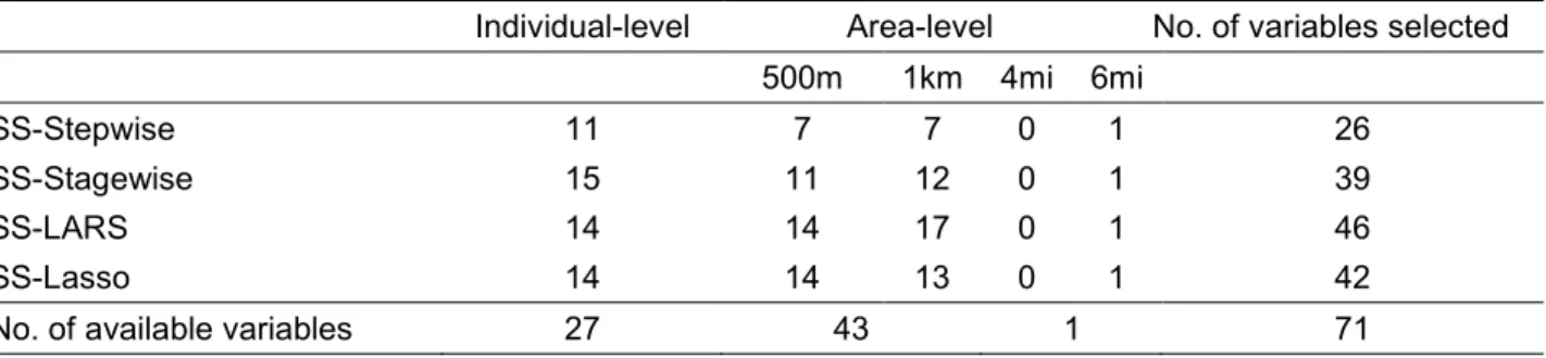
variables and the area-based variables considered at multiple spatial scales. ... 37 2.3. Number of variables selected at each spatial scale for spatial scale (SS) forward

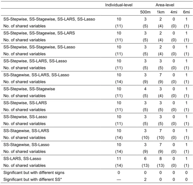
stepwise, forward stagewise, LARS, and lasso models. The last row gives the total number of possible variables at each spatial scale. ... 39 2.4. Number of shared significant variables with the same sign and spatial scale and

total number of shared variables for spatial scale (SS) forward stepwise, forward stagewise, LARS, and lasso models. The frequency of shared significant variables with the same sign and spatial scale is given along with the total number of shared

(11)

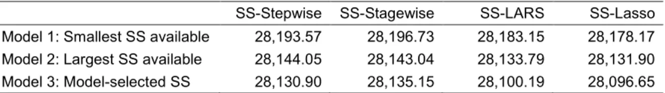
ix 2.5. OLS-based Akaike Information Criterion (AIC) comparisons across spatial scale

(SS) forward stepwise, forward stagewise, LARS, and lasso models. ... 41 3.1. Variable definitions for the variables considered in the spatial scale forward

stepwise, forward stagewise, LARS, and lasso models. The horizontal dashed line separates the individual-level variables and the neighborhood-level variables available at more than one spatial scale. Any variable that falls below the dashed

line has a suffix indicating the associated spatial scale. ... 51 3.2. Number of covariates selected at each spatial scale (SS) by SS forward stepwise,

forward stagewise, and LARS/lasso models. The last row gives the total number of possible variables at each spatial scale. ... 56 3.3. Standardized coefficient estimates from spatial scale (SS) forward stepwise,

forward stagewise, LARS, and lasso models of BMIZ. The blank cells indicate variables not selected for a particular model. The horizontal dashed line separates the individual-level variables and the neighborhood-level variables considered at

multiple spatial scales. ... 60 3.4. OLS-based Akaike information criterion (AIC) comparisons across spatial scale

(SS) forward stepwise, forward stagewise, and LARS/lasso models. ... 61 3.5. Standardized coefficient estimates from the spatial scale (SS) forward stepwise

model of BMIZ with no random effect (RE) in contrast to standardized coefficient estimates from three mixed models with a RE at the census block group (CBG), RE at the census tract (CT), and RE at the CBG and CT. The mixed models were fit using the covariates that were chosen by the SS stepwise algorithm. The horizontal dashed line separates the individual-level variables and the neighborhood-level

variables considered at multiple spatial scales. ... 62 3.6. Standardized coefficient estimates from the spatial scale (SS) forward stagewise

model of BMIZ with no random effect (RE) in contrast to standardized coefficient estimates from three mixed models with a RE at the census block group (CBG), RE at the census tract (CT), and RE at the CBG and CT. The mixed models were fit using the covariates that were chosen by the SS stagewise algorithm. The horizontal dashed line separates the individual-level variables and the

neighborhood-level variables considered at multiple spatial scales. ... 63 3.7. Standardized coefficient estimates from the spatial scale (SS) LARS/lasso model of

BMIZ with no random effect (RE) in contrast to standardized coefficient estimates from three mixed models with a RE at the census block group (CBG), RE at the census tract (CT), and RE at the CBG and CT. The mixed models were fit using the covariates that were chosen by the SS LARS/lasso algorithm. The horizontal

dashed line separates the individual-level variables and the neighborhood-level

(12)

x 3.8. AIC comparisons among spatial scale (SS) forward stepwise, forward stagewise,

and LARS/lasso models with varying random effects (RE): no RE, RE at CBG, RE at CT, and RE at CBG and CT. ... 66 3.9. Standardized coefficient estimates when the covariate male and covariates selected

by the spatial scale (SS) forward stepwise, forward stagewise, and LARS/lasso algorithms were plugged into OLS regression models of BMIZ. The blank cells indicate variables not selected for a particular model. The horizontal dashed line separates the individual-level variables and the neighborhood-level variables

considered at multiple spatial scales. ... 67 3.10. Standardized coefficient estimates when the covariate male, select interaction terms,

and covariates selected by the spatial scale (SS) forward stepwise, forward

stagewise, and LARS/lasso algorithms were plugged into OLS regression models of BMIZ. The blank cells indicate variables not selected for a particular model. The horizontal dashed line separates the individual-level variables and the

neighborhood-level variables considered at multiple spatial scales. ... 68 3.11. Reference table for interpretation of the slopes under four different conditions,

where different signs are realized by coefficient estimates for a continuous main

effect (β�2) and an interaction (β�12)... 69 3.12. Standardized coefficient estimates when the covariate male, select interaction terms,

and covariates selected by the spatial scale forward stepwise algorithm were plugged into an OLS regression model of BMIZ with no random effect (RE) in contrast to coefficient estimates from three mixed models with a RE at the census block group (CBG), RE at the census tract (CT), and RE at the CBG and CT. The horizontal dashed line separates the individual-level variables and the

neighborhood-level variables considered at multiple spatial scales. ... 71 3.13. Standardized coefficient estimates when the covariate male, select interaction terms,

and covariates selected by the spatial scale forward stagewise algorithm were plugged into an OLS regression model of BMIZ with no random effect (RE) in contrast to coefficient estimates from three mixed models with a RE at the census block group (CBG), RE at the census tract (CT), and RE at the CBG and CT. The horizontal dashed line separates the individual-level variables and the

neighborhood-level variables considered at multiple spatial scales. ... 72 3.14. Standardized coefficient estimates when the covariate male, select interaction terms,

and covariates selected by the spatial scale LARS/lasso algorithm were plugged into an OLS regression model of BMIZ with no random effect (RE) in contrast to

coefficient estimates from three mixed models with a RE at the census block group (CBG), RE at the census tract (CT), and RE at the CBG and CT. The horizontal dashed line separates the individual-level variables and the neighborhood-level

(13)

xi 3.15. AIC comparisons among SS forward stepwise-, SS forward stagewise-, and SS

LARS/lasso-based models with interactions and varying random effects (RE): no

RE, RE at CBG, RE at CT, and RE at CBG and CT. ... 75 4.1. Variable definitions for the variables considered in the simulation studies. The

horizontal dashed line separates the individual-level variables and the area-level

variables available at more than one spatial scale. ... 82 4.2. Overview table of simulation study designs. ... 86 4.3. Select coefficient estimates under the second scenario for simulation study 2 for

two forward stagewise approaches, specifically spatial scale (SS) forward stagewise and standard forward stagewise. Variables of interest for this case study are

italicized. ... 91 4.4. MSE calculations for percent vacant at the CBG and CT levels for the spatial scale

(SS) forward stagewise and standard stagewise approaches. ... 92 4.5. Additive MSE calculations for the combined effect of percent vacant for the spatial

scale (SS) forward stagewise and standard stagewise approaches. ... 93 4.6. Average sensitivity and average specificity over the covariates for stepwise

simulation studies 1–6. Cells with no information are denoted by a —. ... 96 4.7. Power and Type I error of the additive test across CBG only, CT only, SS stepwise,

not SS stepwise, LARS stepwise, and step package methods for simulation study 1. Type I errors are italicized. ... 102 4.8. Power of the additive test across CBG only, CT only, SS stepwise, not SS stepwise,

LARS stepwise, and step package methods for simulation study 6. ... 104 4.9. Average sensitivity and average specificity across the covariates for stagewise

simulation studies 1–6. Cells with no information are denoted by a —. ... 107 4.10. Power and Type I error of the additive test across census block group (CBG) only,

census tract (CT) only, spatial scale (SS) stagewise, not SS stagewise, and LARS

stagewise methods for simulation study 1. Type I errors are italicized. ... 113 4.11. Power of the additive test across census block group (CBG) only, census tract (CT)

only, spatial scale (SS) stagewise, not SS stagewise, and LARS stagewise methods for simulation study 6. ... 115 4.12. Average sensitivity and average specificity across the covariates for LARS

simulation studies 1–6. Cells with no information are denoted by a —. ... 118 4.13. Power and Type I error of the additive test across census block group (CBG) only,

census tract (CT) only, spatial scale (SS) LARS, and LARS methods for simulation study 1. Type I errors are italicized. ... 124

(14)

xii 4.14. Power of the additive test across census block group (CBG) only, census tract (CT)

only, spatial scale (SS) LARS, and LARS methods for simulation study 6. ... 126 4.15. Average sensitivity and average specificity across the covariates for lasso

simulation studies 1–6. Cells with no information are denoted by a —. ... 128 4.16. Average sensitivity and average specificity across the covariates for spatial scale

(SS) stepwise, SS stagewise, SS LARS, and SS lasso simulation studies 1–6. Cells with no information are denoted by a —. ... 131 4.17. Power and Type I error of the additive test across spatial scale (SS) stepwise, SS

stagewise, SS LARS, and SS lasso approaches for simulation study 1. Type I errors are italicized. ... 135 4.18. Power of the additive test across spatial scale (SS) stepwise, SS stagewise, SS

LARS, and SS lasso approaches for simulation study 6. ... 136 5.1. Potential areas of further study. ... 146 A.1. Sensitivity and specificity of variable selection for census block group (CBG) only,

census tract (CT) only, spatial scale (SS), not SS stepwise, LARS stepwise, and step package approaches under six different scenarios for simulation study 1.

Specificity values are italicized. ... 185 A.2. Sensitivity and specificity of variable selection for census block group (CBG) only,

Specificity values are italicized. ... 194 A.6. Sensitivity and specificity of variable selection for CBG only, CT only, spatial scale

(SS), not SS stepwise, LARS stepwise, and step package approaches under six

(15)

xiii A.7. Power and Type I error of the additive test across CBG only, CT only, SS stepwise,

not SS stepwise, LARS stepwise, and step package methods for simulation study 1. Type I errors are italicized. ... 197 A.8. Power of the additive test across CBG only, CT only, SS stepwise, not SS stepwise,

LARS stepwise, and step package methods for simulation study 6. ... 199 A.9. Sensitivity and specificity of variable selection for census block group (CBG) only,

census tract (CT) only, spatial scale (SS), not SS stagewise, and LARS stagewise approaches under six different scenarios for simulation study 1. Specificity values are italicized. ... 200 A.10. Sensitivity and specificity of variable selection for census block group (CBG) only,

census tract (CT) only, spatial scale (SS), not SS stagewise, and LARS stagewise approaches under six different scenarios for simulation study 6. Specificity values are italicized. ... 210 A.15. Power and Type I error of the additive test across census block group (CBG) only,

census tract (CT) only, spatial scale (SS) stagewise, not SS stagewise, and LARS

stagewise methods for simulation study 1. Type I errors are italicized. ... 211 A.16. Power of the additive test across census block group (CBG) only, census tract (CT)

only, spatial scale (SS) stagewise, not SS stagewise, and LARS stagewise methods for simulation study 6. ... 213 A.17. Sensitivity and specificity of variable selection for census block group (CBG) only,

census tract (CT) only, spatial scale (SS) LARS, and LARS approaches under six

(16)

xiv A.18. Sensitivity and specificity of variable selection for census block group (CBG) only,

different scenarios for simulation study 2. Specificity values are italicized... 216 A.19. Sensitivity and specificity of variable selection for census block group (CBG) only,

different scenarios for simulation study 6. Specificity values are italicized... 224 A.23. Power and Type I error of the additive test across census block group (CBG) only,

census tract (CT) only, spatial scale (SS) LARS, and LARS methods for simulation study 1. Type I errors are italicized. ... 225 A.24. Power of the additive test across census block group (CBG) only, census tract (CT)

only, spatial scale (SS) LARS, and LARS methods for simulation study 6. ... 227 A.25. Sensitivity and specificity of variable selection for census block group (CBG) only,

census tract (CT) only, spatial scale (SS) lasso, and lasso approaches under six

(17)

xv A.30. Sensitivity and specificity of variable selection for census block group (CBG) only,

different scenarios for simulation study 6. Specificity values are italicized... 238 A.31. Power and Type I error of the additive test across census block group (CBG) only,

census tract (CT) only, spatial scale (SS) lasso, and lasso methods for simulation

study 1. Type I errors are italicized. ... 239 A.32. Power of the additive test across census block group (CBG) only, census tract (CT)

only, spatial scale (SS) lasso, and lasso methods for simulation study 6. ... 241 A.33. Sensitivity and specificity of variable selection for spatial scale (SS) stepwise, SS

stagewise, SS LARS, and SS lasso approaches under six different scenarios for

simulation study 1. Specificity values are italicized. ... 242 A.34. Sensitivity and specificity of variable selection for spatial scale (SS) stepwise, SS

simulation study 6. Specificity values are italicized. ... 252 A.39. Power and Type I error of the additive test across spatial scale (SS) stepwise, SS

stagewise, SS LARS, and SS lasso approaches for simulation study 1. Type I errors are italicized. ... 253 A.40. Power of the additive test across spatial scale (SS) stepwise, SS stagewise, SS

(18)

xvi

LIST OF FIGURES

Figure Page

2.1. Coefficient paths for spatial scale forward stepwise regression to explain log nitrate concentration in drinking wells in Iowa. The scale the variable entered

the model is indicated by the legend. ... 33 2.2. Coefficient paths for spatial scale incremental forward stagewise regression to

explain log nitrate concentration in drinking wells in Iowa. The scale the variable entered the model is indicated by the legend. ... 34 2.3. Coefficient paths for spatial scale LARS to explain log nitrate concentration in

drinking wells in Iowa. The scale the variable entered the model is indicated by the legend. The dotted vertical line indicates the chosen model that had the

minimum OLS-based AIC. ... 35 2.4. Coefficient paths for spatial scale lasso to explain log nitrate concentration in

drinking wells in Iowa. The scale the variable entered the model is indicated by the legend. The dotted vertical line indicates the chosen model that had the

minimum OLS-based AIC. ... 36 3.1. Three levels of influence (individual, familial, and community) that impact a

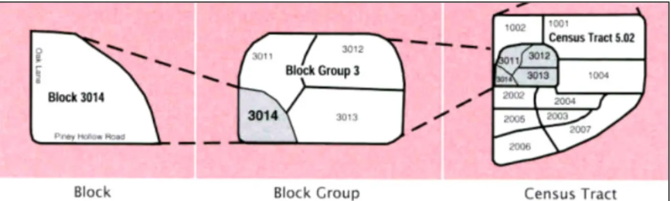
child’s weight status. Reproduced from Davison and Birch (2001). ... 48 3.2. Schematic of nested census boundaries: census block, census block group, and

census tract. Reproduced from U.S. Census Bureau (2001). ... 50 3.3. Choropleth map of average BMIZ by census tract. The selected area shown is

the Richmond Metropolitan Statistical Area (MSA). ... 52 3.4. Choropleth map of population density by census tract. The selected area shown

is the Richmond Metropolitan Statistical Area (MSA)... 52 3.5. Choropleth map of crimes against persons index by census tract. The selected

(19)

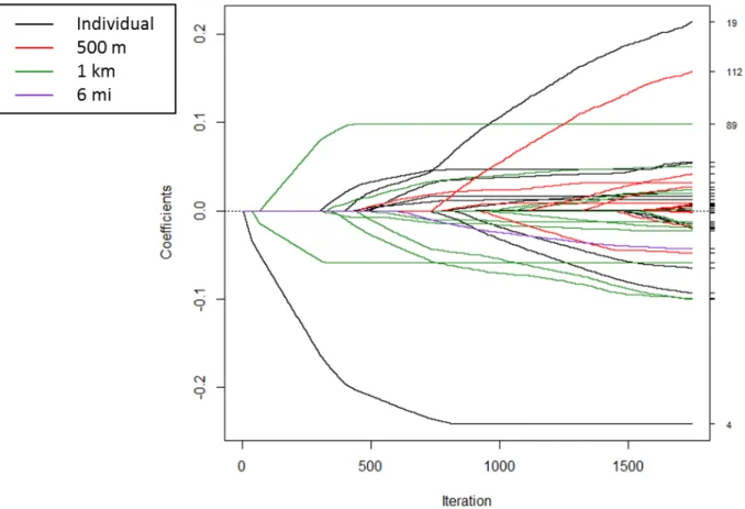
xvii 3.6. Coefficient paths for spatial scale forward stepwise regression to explain BMIZ.

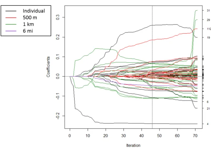
The scale at which each covariate entered the model is indicated by the legend. The numbers on the right-hand side of the figure are the variable numbers as listed in Table 3.1. ... 57 3.7. Coefficient paths for spatial scale incremental forward stagewise regression to

explain BMIZ. The scale at which each covariate entered the model is indicated by the legend. The numbers on the right-hand side of the figure are the variable

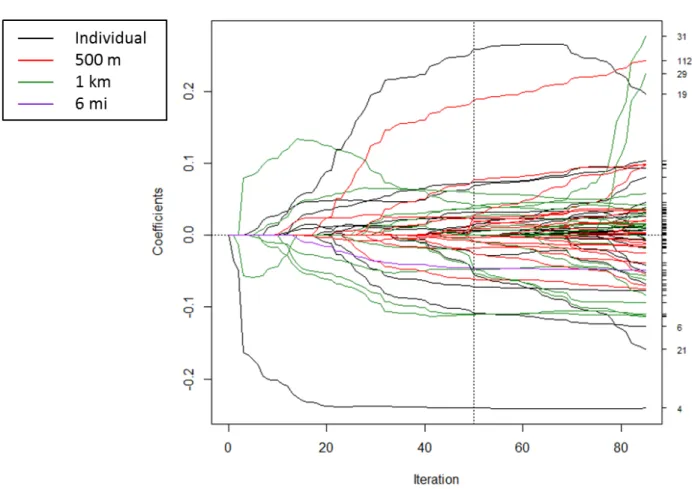
numbers as listed in Table 3.1. ... 58 3.8. Coefficient paths for spatial scale LARS/lasso to explain BMIZ. The scale at

which each covariate entered the model is indicated by the legend. The numbers on the right-hand side of the figure are the variable numbers as listed in Table 3.1. The dotted vertical line indicates the chosen model that had the minimum OLS-

based AIC... 59 3.9. Maps of random effects at the census block group (CBG), census tract (CT), and

CBG/CT for linear mixed-effects models of BMIZ using covariates selected by the spatial scale (SS) forward stepwise, forward stagewise, and LARS/lasso algorithms. The selected area shown is the Richmond Metropolitan Statistical Area (MSA). ... 65 3.10. Maps of random effects at the census block group (CBG), census tract (CT), and

CBG/CT for linear mixed-effects models of BMIZ using covariates selected by the spatial scale (SS) forward stepwise, forward stagewise, and LARS/lasso algorithms, respectively; the covariate male; and select interaction terms. The selected area

shown is the Richmond Metropolitan Statistical Area (MSA). ... 74 4.1. The chosen study area for each simulated dataset was the Richmond Metropolitan

Statistical Area (MSA), here divided into census tracts and featuring all 23,130

patient locations. ... 81 4.2. Spearman correlation coefficients across socioeconomic variables at the census

block group and census tract levels. Correlation coefficients with a magnitude

greater than 0.6 are highlighted in red. ... 84 4.3. Average specificity values across the covariates for each of the six stepwise

approaches for each scenario of simulation studies 1–6. ... 94 4.4. Mean additive MSE values of the coefficient estimates for six different forward

stepwise modeling approaches from simulation study 1. The bottom panel restricts the y-axis to (0.0003, 0.0006) and excludes the CBG only method in order to show in detail the results from the five other methods. The spatial scale (SS) stepwise

and the standard stepwise (not SS) results overlay one another. ... 98 4.5. Mean additive MSE values of the coefficient estimates for six different forward

stepwise modeling approaches from simulation study 5. The bottom panel restricts the y-axis to (0.0002, 0.0005) and excludes the CBG and CT only methods in order to show in detail the results from the four other methods... 99

(20)

xviii 4.6. Mean additive MSE values of the coefficient estimates for six different forward

stepwise modeling approaches from simulation study 6. The bottom panel restricts the y-axis to (-0.0952, 2.4951) and excludes the CT only method in order to show in detail the results from the five other methods... 100 4.7. Mean additive MSE values of the coefficient estimates for five different forward

stagewise modeling approaches from simulation study 1. The bottom panel restricts the y-axis to (0.0002, 0.0021) and excludes the CBG only method in order to show in detail the results from the four other methods. The CT only, spatial scale (SS)

stagewise, and standard stagewise (not SS) results overlay one another. ... 109 4.8. Mean additive MSE values of the coefficient estimates for five different forward

stagewise modeling approaches from simulation study 4. The bottom panel restricts the y-axis to (-0.0185, 0.4879) and excludes the CBG and CT only methods in order to show in detail the results from the three other methods. ... 110 4.9. Mean additive MSE values of the coefficient estimates for five different forward

stagewise modeling approaches from simulation study 6... 111 4.10. Mean additive MSE values of the coefficient estimates for four different LARS

modeling approaches from simulation study 1. The bottom panel restricts the y-axis to (0.0002, 0.0018) and excludes the CBG only method in order to show in detail the results from the three other methods. The CT only and spatial scale

(SS) LARS results overlay one another. ... 120 4.11. Mean additive MSE values of the coefficient estimates for four different LARS

modeling approaches from simulation study 5. ... 121 4.12. Mean additive MSE values of the coefficient estimates for four different LARS

modeling approaches from simulation study 6. The bottom panel restricts the y-axis to (-0.0924, 2.4213) and excludes the CT only method in order to show

in detail the results from the three other methods. ... 122 4.13. Mean additive MSE values of the coefficient estimates for four different spatial

scale (SS) modeling approaches from simulation study 1. The bottom panel restricts the y-axis to (0.0003, 0.0004) and excludes the SS stagewise method in order to show in detail the results from the three other methods. The SS LARS

and SS lasso results overlay one another. ... 133 4.14. Mean additive MSE values of the coefficient estimates for four different spatial

scale (SS) modeling approaches from simulation study 4. The SS LARS and

SS lasso results overlay one another. ... 134 4.15. Mean additive MSE values of the coefficient estimates for four different spatial

(21)

xix A.1. Mean additive MSE values of the coefficient estimates for six different forward

stepwise modeling approaches from simulation study 1. The bottom panel restricts the y-axis to (0.0003, 0.0006) and excludes the CBG only method in order to show in detail the results from the five other methods. The spatial scale (SS) stepwise

and the standard stepwise (not SS) results overlay one another. ... 155 A.2. Mean additive MSE values of the coefficient estimates for six different forward

stepwise modeling approaches from simulation study 2. The bottom panel restricts the y-axis to (0.0003, 0.0006) and excludes the CBG and CT only methods in order to show in detail the results from the four other methods... 156 A.3. Mean additive MSE values of the coefficient estimates for six different forward

stepwise modeling approaches from simulation study 6. The bottom panel restricts the y-axis to (-0.0952, 2.4951) and excludes the CT only method in order to show in detail the results from the five other methods... 160 A.7. Mean additive MSE values of the coefficient estimates for five different forward

stagewise modeling approaches from simulation study 1. The bottom panel restricts the y-axis to (0.0002, 0.0021) and excludes the CBG only method in order to show in detail the results from the four other methods. The CT only, spatial scale (SS)

stagewise, and standard stagewise (not SS) results overlay one another. ... 161 A.8. Mean additive MSE values of the coefficient estimates for five different forward

stagewise modeling approaches from simulation study 2. The bottom panel restricts the y-axis to (-0.0002, 0.0072) and excludes the CBG and CT only methods in order to show in detail the results from the three other methods. ... 162 A.9. Mean additive MSE values of the coefficient estimates for five different forward

stagewise modeling approaches from simulation study 3. The bottom panel restricts the y-axis to (-0.0031, 0.0874) and excludes the CBG and CT only methods in order to show in detail the results from the three other methods. ... 163

(22)

xx A.10. Mean additive MSE values of the coefficient estimates for five different forward

stagewise modeling approaches from simulation study 6... 166 A.13. Mean additive MSE values of the coefficient estimates for four different LARS

modeling approaches from simulation study 1. The bottom panel restricts the y-axis to (0.0002, 0.0018) and excludes the CBG only method in order to show in detail the results from the three other methods. The CT only and spatial scale (SS) LARS results overlay one another. ... 167 A.14. Mean additive MSE values of the coefficient estimates for four different LARS

modeling approaches from simulation study 2. The bottom panel restricts the y-axis to (-7.54e-05, 9.34e-03) and excludes the CBG and CT only methods in

order to show in detail the results from the two other methods. ... 168 A.15. Mean additive MSE values of the coefficient estimates for four different LARS

modeling approaches from simulation study 3. The bottom panel restricts the y-axis to (-0.0366, 0.9578) and excludes the CBG and CT only methods in

modeling approaches from simulation study 5. ... 171 A.18. Mean additive MSE values of the coefficient estimates for four different LARS

in detail the results from the three other methods. ... 172 A.19. Mean additive MSE values of the coefficient estimates for four different lasso

modeling approaches from simulation study 1. The bottom panel restricts the y-axis to (0.0002, 0.0018) and excludes the CBG only method in order to show

(23)

xxi A.20. Mean additive MSE values of the coefficient estimates for four different lasso

modeling approaches from simulation study 2. The bottom panel restricts the y-axis to (-7.54e-05, 9.34e-03) and excludes the CBG and CT only methods in

order to show in detail the results from the two other methods. ... 174 A.21. Mean additive MSE values of the coefficient estimates for four different lasso

modeling approaches from simulation study 5. ... 177 A.24. Mean additive MSE values of the coefficient estimates for four different lasso

in detail the results from the three other methods. ... 178 A.25. Mean additive MSE values of the coefficient estimates for four different spatial

scale (SS) modeling approaches from simulation study 1. The bottom panel restricts the y-axis to (0.0003, 0.0004) and excludes the SS stagewise method in order to show in detail the results from the three other methods. The SS LARS

and SS lasso results overlay one another. ... 179 A.26. Mean additive MSE values of the coefficient estimates for four different spatial

SS lasso results overlay one another. ... 180 A.27. Mean additive MSE values of the coefficient estimates for four different spatial

(24)

xxii

ABSTRACT

SELECTING SPATIAL SCALE OF AREA-LEVEL COVARIATES IN REGRESSION MODELS

By Lauren P. Grant, Ph.D.

A dissertation submitted in partial fulfillment of the requirements for the degree of Doctor of Philosophy at Virginia Commonwealth University.

Virginia Commonwealth University, 2016 Director: David C. Wheeler, Ph.D., MPH Assistant Professor, Department of Biostatistics

Director: Chris Gennings, Ph.D.

Research Professor, Department of Preventive Medicine Icahn School of Medicine at Mount Sinai

In epidemiological and environmental studies, investigators are often interested in the contextual or area-level effects that are associated with a specific health outcome. Area-based covariates are typically available at multiple spatial scales (i.e., areal units or buffer distances). Studies have found that the level of association between an area-level covariate and an outcome can vary depending on the spatial scale (SS) of a particular covariate. However, covariates used in regression models are customarily modeled at the same spatial unit. In this dissertation, we developed four SS model selection algorithms that select the best spatial scale for each area-level covariate. The SS forward stepwise, SS incremental forward stagewise, SS least angle

(25)

xxiii covariates at different spatial scales, while constraining each covariate to enter at most one spatial scale. We applied our methods to two real applications with area-level covariates available at multiple scales to model variation in the following outcomes: 1) nitrate

concentrations in private wells in Iowa and 2) body mass index z-scores of pediatric patients of the Virginia Commonwealth University Medical Center. In both applications, our SS algorithms selected covariates at different spatial scales, producing a better goodness of fit in comparison to traditional models, where all area-level covariates were modeled at the same scale. We

evaluated our methods using simulation studies to examine the performance of our SS algorithms in relation to existing methods and to one another. As our primary comparison, we evaluated the performance of our SS approaches with that of traditional modeling approaches, where all covariates entered at a common scale, and determined that the SS algorithms generally outperformed the conventional approaches. These findings underscore the importance of considering spatial scale when performing model selection. Our techniques can be generalized to other spatial scale model selection problems, where it is of interest to investigate the

relationship between covariates available at multiple spatial scales and a particular outcome of interest.

(26)

1 CHAPTER 1

INTRODUCTION

1.1 BACKGROUND

In the realm of public health research, it has been well established that geographic

location plays an important role in influencing health outcomes (Diez Roux, 2001; Flowerdew et al., 2008; Kawachi & Berkman, 2003; Krieger et al., 2002, 2003; Root, 2012; Root et al., 2011). Investigators frequently use contextual or area-level covariates in regression models to help capture area-based characteristics of an individual’s surrounding environment, such as percent of population that lives below the federal poverty line. To obtain area-based variables, researchers can use geocoding in a geographic information system (GIS) to match a person’s residential address to an external database that houses many area-level variables, each of which is often available at more than one spatial scale or geographic unit. For instance, socioeconomic status (SES) variables from the U.S. Census are available at several scales: census block group, census tract, county, and state. This abundance of area-level data raises the following research

question—at which spatial scale should each area-level covariate be modeled in order to explain a particular outcome variable of interest?

In the literature, various studies have been conducted to consider spatial scale when modeling associations between area-level variables and health outcomes (Flowerdew et al.,

(27)

2

2008; Krieger et al., 2002, 2003; Root, 2012; Root et al., 2011). Traditionally, area-based covariates in regression models are assumed to all be appropriately modeled at the same spatial scale, where the general rule of thumb is that smaller is better in terms of the chosen spatial unit (Krieger et al., 2002, 2003; Toprani & Hadler, 2013). However, some studies have shown that different area-level covariates are associated with outcomes at different spatial scales (Crowder & South, 2011; Flowerdew et al., 2008; Root, 2012; Root et al., 2011; Rupert, 2003). As an example, Root (2012) finds that the strength of association between area-level SES covariates and orofacial cleft risk changes when using different spatial scales (i.e., 4000-meter buffer, census tract, census block group) and that poverty and unemployment have a stronger relationship with risk for cleft palate at smaller and larger scales, respectively.

1.2 MOTIVATION

Given that area-level covariates appear to have different effects at different scales, we seek an alternative to the conventional approach of choosing one spatial scale at which to model all area-level covariates. Rather, we opt to allow each area-level variable to enter a model at one or more spatial scales. However, in cases of highly correlated variables, this type of allowance could be problematic as we will demonstrate.

As a motivational example, we modeled the relationship between body mass index z -score and various individual-level and neighborhood-level covariates available at multiple spatial scales. The study population (n = 27,987) consisted of children, ranging from 2 to 17 years of age, who visited the Virginia Commonwealth University (VCU) Medical Center from 2009 to 2012. We used incremental forward stagewise regression, a forward model selection approach where each neighborhood-level variable was allowed to enter the model at more than one spatial unit. As a result, we saw many area-level covariates included at multiple spatial scales in the

(28)

3

model. Coefficient estimates and the associated ordinary least squares (OLS) estimates are given in Table 1.1.

The highlighted coefficient estimates indicate variables whose estimates were in opposite directions (i.e., positive and negative). For example, population density had a positive

association at the census block level (CBK), but negative associations at the census block group (CBG) and census tract levels (CT). Similarly, many of the crime indices expressed conflicting estimates at the block group and tract levels.

Overall, we can largely attribute the conflicting estimates to be a consequence of collinearity. If covariates are highly correlated, it is not uncommon to see corresponding estimates with opposite signs (Hastie et al., 2009; Hill & Adkins, 2003; Stolzenberg, 2004). When we separately modeled each area-level crime index covariate, they shared common signs; yet when we jointly modeled the crime covariates, they had opposite signs. This reversal paradox is a classic indicator of collinearity.

(29)

4

Table 1.1. Standardized coefficient estimates for variables in a forward stagewise regression model of body mass index z-score (BMIZ). Variables selected by the stagewise algorithm were used in an ordinary least squares (OLS) regression model to obtain p-values. Conflicting estimates (i.e., estimates with opposite signs at different spatial scales) are boldfaced and italicized. The horizontal dashed line separates the individual-level variables and the area-level variables available at more than one spatial scale.

Explanatory Variable Stagewise OLS

Visit Age 0.079 0.080 (*) Male _{-0.002 -0.003} Black 0.040 0.040 (*) Population Density_CBK 0.003 0.004 Population Density_CBG -0.015 -0.020 (+) Population Density_CT -0.027 -0.021 (+) % White_CT _{-0.018 -0.021} % Hispanic White_CBG _{0.020 0.018} % Hispanic White_CT 0.020 0.024 (+) % Hispanic Black_CBG _{0.005 0.009} % Hispanic Black_CT _{0.010 0.005} Median Household Income_CBG -0.032 -0.034 (*) Median Household Income_CT -0.058 -0.058 (*)

% Renter_CT -0.037 -0.042 (*) % Vacant_CT 0.015 0.015 (*) Murder Index_CBG -0.055 -0.084 (*) Murder Index_CT 0.031 0.062 (*) Rape Index_CBG 0.021 0.037 (*) Rape Index_CT -0.002 -0.020 Robbery Index_CBG -0.008 -0.039 (+) Robbery Index_CT 0.005 0.039 Assault Index_CBG -0.027 -0.037 (+) Assault Index_CT 0.026 0.036 Burglary Index_CT _{0.004 0.007} Larceny Index_CBG 0.011 0.022 Larceny Index_CT -0.019 -0.033 (+) Motor Vehicle Theft Index_CBG 0.019 0.051 (*) Motor Vehicle Theft Index_CT -0.032 -0.068 (*) Notes: Values marked with (*) have a p-value < 0.05, and values marked with (+) have an associated p-value < 0.1.

CBK = census block, CBG = census block group, CT = census tract

As described in Table 1.2, the area-level covariates were highly correlated across spatial scales. The correlation coefficients ranged from a minimum of 0.74 to a maximum of 0.97,

(30)

5

demonstrating strong correlations were present between covariates across different spatial units. In light of this, it is not surprising to see collinearity problems as a result of modeling the same covariate at more than one spatial scale.

Table 1.2. Spearman correlation coefficients between neighborhood covariates across different spatial scales. Variable ρCBG,CT ρCBK,CBG ρCBK,CT Population Density 0.90 0.78 0.74 % White 0.96 — — % Hispanic White 0.88 — — % Hispanic Black 0.83 — —

Median Household Income 0.93 — —

% Renter 0.85 — — % Vacant 0.87 — — Murder Index 0.96 — — Rape Index 0.95 — — Robbery Index 0.97 — — Assault Index 0.96 — — Burglary Index 0.96 — — Larceny Index 0.94 — —

Motor Vehicle Theft Index 0.96 — — Note: CBK = census block, CBG = census block group, CT = census tract

The potential negative ramifications of modeling an area-level covariate at multiple spatial scales calls for the need to model each area-level variable at a single spatial unit. Yet the traditional approach of modeling all contextual covariates at the same spatial scale does not take into account that different area-level variables can be influential at different scales. Hence, we have taken measures to address this problem through the development of four spatial scale (SS) model selection algorithms, where all area-level variables are considered at all available scales to enter a model, but each area-level covariate is constrained to enter the model at a single spatial scale.

(31)

6

1.3 PROSPECTUS

The remainder of this dissertation is organized into four parts or chapters. Chapter 2 is based on a published paper (Grant et al., 2015) and includes the development of the SS forward stepwise, SS incremental forward stagewise, SS least angle regression (LARS), and SS lasso algorithms and an environmental application modeling groundwater nitrate concentrations in Iowa. Chapter 3 features a socioeconomic application of our SS methods to a pediatric body mass index (BMI) dataset and additionally considers interactions and random effects at different spatial scales. Chapter 4 investigates various simulation study scenarios comparing model performance of different approaches (e.g., selecting each covariate at only one SS or at more than one SS) in addition to comparing model performance across SS algorithms. Chapter 5 summarizes our work and discusses areas for potential future work. Following Chapter 5,

appendices provide supplemental material for Chapter 4 (Appendix A), R code for an example of how to preprocess the data prior to implementation of the SS algorithms (Appendix B), and the R code for the SS algorithms (Appendix C).

(32)

7 CHAPTER 2

SELECTING SPATIAL SCALE OF COVARIATES IN REGRESSION

MODELS OF ENVIRONMENTAL EXPOSURES1

2.1 INTRODUCTION

In public health research, it is acknowledged that both compositional (individual-level) and contextual (neighborhood-level) variables are important for explaining variation in health outcomes (Diez Roux, 2003; Flowerdew et al., 2008; Kawachi & Berkman, 2003; Krieger et al., 2002, 2003; Root, 2012; Root et al., 2011). For example, the role of contextual variables

continues to be a key focus of investigators studying potential risk factors for obesity (Block et al., 2004; Galvez et al., 2010; Prince et al., 2011), where neighborhood variables such as fast food density and green space presence are thought to be important factors that contribute to obesity status. Neighborhood- or area-level variables can also have an important role in

explaining variation in environmental chemical exposures. One example is found with modeling variation in polychlorinated biphenyls (PCBs) measured in carpet dust using percentage of developed land, population density, and number of industrial facilities within 2 kilometers (km) of residences, where total PCB levels are significantly associated with either percentage of developed land or population density (DellaValle et al., 2013).

1_{This chapter previously appeared as an article in}_{Cancer Informatics}_{. The original citation is as follows: Grant, L.,}

Gennings, C., & Wheeler, D. C. (2015). Selecting spatial scale of covariates in regression models of environmental exposures. Cancer Informatics, 14(S2), 81–96.

(33)

8

Through the use of geocoding and geographic information systems (GIS), researchers can link an individual residential address to an external database containing numerous area-level or environmental variables, where the number of variables is denoted by p. Typically, each of the area-level variables is available at multiple geographic scales. Thus, the p number of area-level variables available to consider when explaining variation in a health outcome can quickly multiply. Many socioeconomic variables, including race, education, household income, and housing tenure, are available from the U.S. Census at the census block group, census tract, and county level. To clarify, we use the word “level” as a general term for spatial unit. Level is synonymous with region size, which, as will be seen later in our case example, denotes a buffer size. In addition to geopolitical areas, researchers can also create a set of geographic areas of varying size to summarize environmental variables using circular buffers or rings centered at observed data points. As an example, population density can be calculated at distances of one, two, and three miles (mi) from a residential location by intersecting spatial buffers of these sizes with census block group data.

With the abundance of socioeconomic and environmental data available at multiple spatial scales, a natural question arises for researchers who wish to investigate environmental effects—at what spatial scale (geographic areal unit) should each area-level variable be modeled in order to explain a fixed health outcome or environmental exposure of interest? Area-level covariates used as contextual variables in regression models are often in practice modeled at the same spatial scale, where, generally, a smaller spatial unit (i.e., census block group versus a county) is thought to better capture heterogeneity in regression relationships. Krieger et al. (2002) model area-based socioeconomic measures at three spatial scales (census block group, census tract, and ZIP Code) to study mortality outcomes and cancer incidence and find that the

(34)

9

effect estimates for the smaller spatial units (census block group and census tract) are similar, while the effect estimates for the larger spatial unit (ZIP Code) differ and are sometimes in the opposite direction. Krieger et al. (2002) conclude that level of geography is important and recommend the use of socioeconomic variables at a smaller spatial scale, namely census block group or census tract.

The selection of spatial scale for environmental variables is a problem typically encountered in modeling groundwater quality. A variable that is often incorporated into

statistical models of groundwater quality is area land use, as it is known to be one of the factors that can affect water quality. Barringer et al. (1990) find that the use of a circular buffer around a water table well is a simple and effective method for correlating water quality and land use. Regional and national groundwater studies have associated land use near a well with water quality using a fixed circular buffer distance, with 500 meters (m) a common choice and 1 km a less common choice (Gardner & Vogel, 2005; Moran et al., 2007; Nolan et al., 2002; Squillace & Moran, 2007; Squillace et al., 2002). Some researchers have evaluated the univariate correlation of land use variables with groundwater quality. Ferrari and Ator (1995) find

correlations between agricultural land use and nitrate concentrations using circular buffers of 400 m and 800 m. Kolpin (1997) correlates the concentrations of nitrate, alachlor, and atrazine detected in wells with a variety of land use variables using circular buffers ranging in size from 200 m to 2 km. Johnson and Belitz (2009) evaluate a range of circular buffer and wedge sizes in a univariate correlation analysis of urban land use and the occurrence of volatile organic

compounds (VOCs) in groundwater using Kendall’s tau (τ). They find that values of τ are within 10% of one another for circles and wedges ranging in size from 500 m to 2 km, with statistically

(35)

10

significant correlations for all sizes, and conclude that the popular choice of a 500 m circular buffer is adequate for assigning land use variables to a well.

Other researchers have evaluated the buffer distance to select for each type of land use variable to use in a regression model of groundwater quality. Rupert (2003) selects the circular buffer size for land use variables to explain detection of elevated atrazine or desethyl-atrazine (atrazine/DEA) concentrations and elevated concentrations of nitrate using univariate logistic regression. The optimal buffer size is 2 km for agricultural land use variables and 500 m for urban land use variables according to McFadden’s rho-squared, a transformation of the log-likelihood statistic that is designed to imitate the r-squared of linear regression for univariate regression models (Rupert, 2003). The buffer distances of 2 km for agricultural land use variables and 500 m for urban land use variables are then used in multiple logistic regression models of the probability of elevated atrazine/DEA detection and the probability of elevated nitrate detection.

An important question is whether all area-level variables should be modeled at the same spatial scale, as recent studies have shown that different area-level covariates are associated with health outcomes at different spatial scales (Flowerdew et al., 2008; Root, 2012; Root et al., 2011). Root (2012) finds that the relationship between area-level socioeconomic status (SES) variables and orofacial cleft risk varies when using different spatial scales to define

neighborhoods. The study results indicate that poverty has a stronger association with risk for cleft palate at smaller geographic scales, while unemployment has a stronger association at larger scales, thus providing evidence that neighborhood effects operate at different spatial scales. In addition, Flowerdew et al. (2008) demonstrate in a British study of limiting long-term illness (LLTI) that the correlation strength between area-level variables and LLTI can vary depending

(36)

11

on the spatial scale. Stronger correlations are present for LLTI and age group at the smaller Enumeration District (ED) scale, while stronger correlations exist for LLTI and unemployment at the larger ward scale. In another study, Block et al. (2004) examine the relationship between fast-food restaurant density (FFRD) and black and low-income neighborhoods while controlling for various neighborhood variables such as commercial activity and presence of highways, which, in addition to FFRD, are available at two spatial scales (0.5- and 1-mi buffer sizes). They find that while the results for both buffer analyses are similar, the 1 mi buffer analysis leads to a statistically significant association for median household income, perhaps due to a better

capturing of how far people are willing to travel to buy food. In light of these findings, it is important to consider spatial scale for each area-level covariate when studying relationships between environmental variables and a particular outcome variable.

In this paper, we present a novel approach for modeling area-based variables at different spatial scales using four model selection approaches. To demonstrate these methods, we use a nitrate dataset containing numerous geologic and land use variables at different buffer sizes to investigate potential associations with nitrate concentrations in drinking well water.

Contamination of drinking water by nitrate is a growing problem in agricultural areas of the United States, as ingested nitrate can lead to the endogenous formation of N-nitroso compounds, which are potent carcinogens. Our methods are not limited to the case example we present, but can be applied to other area-based variables that are related to cancer.

(37)

12

2.2 METHODS

2.2.1 Statistical Methods

We review four established methods used in model selection: forward stepwise regression, incremental forward stagewise regression, least angle regression (LARS), and the lasso (Hastie et al., 2009). Next, we introduce our modified versions of these algorithms to select spatial scale. Lastly, we present an application of our methods to model groundwater nitrate concentrations in Iowa.

2.2.2 Model Selection Approaches

2.2.2.1Forward Stepwise Regression

Forward stepwise regression is a common approach used for model selection. A description of the forward stepwise regression algorithm detailed by Berk (2008) and Wheeler (2009) is as follows:

(1) Initialize all regression coefficients βˆ1, , βˆp=0, and let r y= , where r denotes the residual vector and y denotes the response vector.

(2) Of the candidate variables, find the predictor xj that has the greatest absolute correlation with the residuals r, and add xj to the working design matrix Xin. (3) Let ˆ ( T ₎1 T _.

in in − in =

β X X X y

(4) Compute the residuals r y y= − ˆ, where yˆ is the vector of fitted values.

(5) Iterate steps (2)–(4) until there is an inadequate improvement in the performance of the model or until all predictors have been added to the model.

(38)

13

For step (5), we consider there to be an inadequate improvement in the model’s performance if the difference in the Akaike Information Criterion (AIC) between the current model and the proposed model is less than epsilon, for some epsilon > 0.

2.2.2.2Incremental Forward Stagewise Regression

Incremental forward stagewise regression is another common approach used for model selection. Hastie et al. (2009) and Hastie et al. (2007) describe the incremental forward stagewise regression algorithm as follows:

(1) Initialize all regression coefficients βˆ1, , βˆp=0, and let r y= , where r denotes the residual vector and y denotes the response vector.

(2) Find the predictor xj that has the greatest absolute correlation with the residuals

r.

(3) Let βˆ_j ←βˆ_j+δ_j, where δ_j = ⋅τ sign corr[ ( , )]r x_j for some step size τ >0.

(4) Let r← −r δjxj.

(5) Iterate steps (2)–(4) until none of the predictors are correlated with the residuals

.

r

For step (5), we consider none of the predictors to be correlated with the residuals if

maxcorr( , )r X is less than a specified tolerance, where the tolerance is some small, positive number.

(39)

14

2.2.2.3Least Angle Regression

Following the notation of Yuan and Lin (2006), the LARS algorithm is described as follows:

(1) Initialize all regression coefficients [0] [0] 1

ˆ _{, ,}_ ˆ_p =_0,

β β and let _r[0]₌ _y_,_where_r[0]

denotes the residual vector at index 0 and y denotes the response vector. Set

1,

i= where i is the index for the current iteration count.

(2) Find the predictor xc among the p possible predictors that has the greatest absolute correlation with the residuals _r[ 1]i− _.

(3) Let the active set i be equal to the corresponding column index of X

associated with the predictor x_c, and add xc to the working design matrix Xi.

(4) Let γ be a p-dimensional vector where all values are set equal to 0. Calculate the current least squares direction γ by updating

[ ]

₍ ₎ 1 [ 1]_. i i i T T i i = X X  − X r −  γ

(5) For every j in X that is not an element of the active set i, calculate αj, the minimum distance needed to move the active regression coefficient(s) in direction

γ until another predictor xjhas as much correlation with the current residuals as the variables in the active set. That is, findαj∈(0,1) such that

2 2 [ 1] [ 1] ( ) ( ) , T i T i j − −αj = j′ − −αj x r Xγ x r Xγ