Parallel Algorithms for Big Data Optimization
Francisco Facchinei, Simone Sagratella, and Gesualdo Scutari
Senior Member, IEEE
Abstract—We propose a decomposition framework for the parallel optimization of the sum of a differentiable function and a (block) separable nonsmooth, convex one. The latter term is usually employed to enforce structure in the solution, typically sparsity. Our framework is very flexible and includes both fully parallel Jacobi schemes and Gauss-Seidel (i.e., sequential) ones, as well as virtually all possibilities “in between” with only a subset of variables updated at each iteration. Our theoretical convergence results improve on existing ones, and numerical results on LASSO and logistic regression problems show that the new method consistently outperforms existing algorithms.
Index Terms—Parallel optimization, Distributed methods, Ja-cobi method, LASSO, Sparse solution.
I. INTRODUCTION
The minimization of the sum of a smooth function,F, and of a nonsmooth (block separable) convex one, G,
min
x∈XV(x)≜F(x) +G(x), (1)
is an ubiquitous problem that arises in many fields of en-gineering, so diverse as compressed sensing, basis pursuit denoising, sensor networks, neuroelectromagnetic imaging, machine learning, data mining, sparse logistic regression, genomics, metereology, tensor factorization and completion, geophysics, and radio astronomy. Usually the nonsmooth term is used to promote sparsity of the optimal solution, which often corresponds to a parsimonious representation of some phenomenon at hand. Many of the aforementioned applications can give rise to extremely large problems so that standard optimization techniques are hardly applicable. And indeed, recent years have witnessed a flurry of research activity aimed at developing solution methods that are simple (for example based solely on matrix/vector multiplications) but yet capable to converge to a good approximate solution in reasonable time. It is hardly possible here to even summarize the huge amount of work done in this field; we refer the reader to the recent works [2]–[17] and books [18]–[20] as entry points to the literature.
However, with big data problems it is clearly necessary to design parallel methods able to exploit the computational power of multi-core processors in order to solve many in-teresting problems. It is then surprising that while sequential solutions methods for Problem (1) have been widely investi-gated, the analysis of parallel algorithms suitable to large-scale
The order of the authors is alphabetic; all the authors contributed equally to the paper.
F. Facchinei and S. Sagratella are with the Dept. of Computer, Control, and Management Engneering, at Univ. of Rome La Sapienza, Rome, Italy. Emails:<facchinei,sagratella>@dis.uniroma1.it
G. Scutari is with the Dept. of Electrical Engineering, at the State Univ. of New York at Buffalo, Buffalo, USA. Email:[email protected]. His work was supported by the USA National Science Foundation under Grants CMS 1218717 and CAREER Award No. 1254739.
Part of this work has been presented at the 2014 IEEE International Conference on Acoustics, Speech, and Signal Processing (ICASSP 2014), Florence, Italy, May 4-9 2014, [1].
implementations lags behind. Gradient-type methods can of course be easily parallelized, but they are known to generally suffer from slow convergence; furthermore, by linearizing F they do not exploit any structure of F, a fact that instead has been shown to enhance convergence speed [21]. However, beyond that, and looking at recent approaches, we are only aware of very few papers that deal with parallel solution methods [9]–[16]. These papers analyze both randomized and deterministic block Coordinate Descent Methods (CDMs); one advantage of the analyses therein is that they provide an interesting (global) rate of convergence. However, i) they are essentially still (regularized) gradient-based methods; ii) they are not flexible enough to include, among other things, very natural Jacobi-type methods (where at each iteration a minimization of the original function is performedin parallel
with respect to all blocks of variables); and iii) except for [10], [11], [13], they cannot deal with a nonconvex F. We refer to Section V for a detailed discussion on current parallel and sequential solution methods for (1).
In this paper, we propose a new, broad, deterministic algorithmic framework for the solution of Problem (1). The essential, rather natural idea underlying our approach is to decompose (1) into a sequence of (simpler) subproblems whereby the function F is replaced by suitable convex ap-proximations; the subproblems can be solved in a parallel
and distributed fashion. Key (new) features of the proposed algorithmic framework are: i) it is parallel, with a degree of parallelism that can be chosen by the user and that can go from a complete parallelism (every variable is updated in parallel to all the others) to the sequential (only one variable is updated at each iteration), covering virtually all the possibilities in “between”; ii) it easily leads to distributed implementations; iii) it can tackle a nonconvex F; iv) it is very flexible and includes, among others, updates based on gradient- or Newton-type approximations; v) it easily allows for inexact solution of the subproblems; vi) it permits the update of only some (blocks of) variables at each iteration (a feature that turns out to be very important numerically); vii) even in the case of the minimization of a smooth, convex function (i.e., F ∈ C1 is
convex and G≡0) our theoretical results compare favorably to state-of-the-art methods.
The proposed framework encompasses a gamut of novel algorithms, offering a lot of flexibility to control iteration complexity, communication overhead, and convergence speed, while converging under the same conditions; these desirable features make our schemes applicable to several different prob-lems and scenarios. Among the variety of new updating rules for the (block) variables we propose, it is worth mentioning a combination of Jacobi and Gauss-Seidel updates, which seems particularly valuable in parallel optimization on multi core/processor architectures; to the best of our knowledge this is the first time that such a scheme is proposed and analyzed. A further contribution of the paper is to implement our
schemes and the most representative ones in the literature over a parallel architecture, the General Compute Cluster of the Center for Computational Research at the State University of New York at Buffalo. Numerical results on LASSO and Logis-tic Regression problems show that our algorithms consistently outperform state-of-the-art schemes.
The paper is organized as follows. Section II formally introduces the optimization problem along with the main assumptions under which it is studied. Section III describes our novel general algorithmic framework along with its con-vergence properties. In Section IV we discuss several instances of the general scheme introduced in Section III. Section V contains a detailed comparison of our schemes with state-of-the-art algorithms on similar problems. Numerical results are presented in Section VI, where we focus on LASSO and Logistic Regression problems and compare our schemes with state-of-the-art alternative solution methods. Finally, Section VII draws some conclusions. All proofs of our results are given in the Appendix.
II. PROBLEMDEFINITION
We consider Problem (1), where the feasible set X =
X1× · · · ×XN is a Cartesian product of lower dimensional
convex setsXi⊆Rni, andx∈Rnis partitioned accordingly:
x = (x1, . . . ,xN), with each xi ∈ Rni; F is smooth
(and not necessarily convex) and G is convex and possibly nondifferentiable, with G(x) =∑N
i=1gi(xi). This formulation
is very general and includes problems of great interest. Below we list some instances of Problem (1).
•G(x) = 0; in this case the problem reduces to the minimiza-tion of a smooth, possibly nonconvex problem with convex constraints.
• F(x) = ∥Ax−b∥2 and G(x) = c∥x∥1, X = Rn, with
A ∈Rm×n, b∈Rm, and c ∈ R++ given constants; this is
the renowned and much studied LASSO problem [2].
• F(x) = ∥Ax−b∥2 and G(x) = c∑N
i=1∥xi∥2,X =Rn,
withA∈Rm×n,b∈Rm, andc∈R
++ given constants; this
is the group LASSO problem [22].
• F(x) = ∑mj=1log(1 +e−aiyTix) and G(x) = c∥x∥1 (or G(x) =c∑Ni=1∥xi∥2), withyi ∈Rn,ai ∈R, andc∈R++
given constants; this is the sparse logistic regression problem [23], [24].
• F(x) = ∑mj=1max{0,1−aiyTix}
2 and G(x) = c∥x∥ 1,
with ai∈ {−1,1}, yi ∈Rn, and c∈R++ given; this is the
ℓ1-regularized ℓ2-loss Support Vector Machine problem [5].
• Other problems that can be cast in the form (1) include the Nuclear Norm Minimization problem, the Robust Principal Component Analysis problem, the Sparse Inverse Covariance Selection problem, the Nonnegative Matrix (or Tensor) Fac-torization problem, see e.g., [25] and references therein. Assumptions. Given (1), we make the following blanket assumptions:
(A1) EachXi is nonempty, closed, and convex;
(A2) F isC1 on an open set containingX;
(A3) ∇F is Lipschitz continuous on X with constantLF;
(A4) G(x) =∑Ni=igi(xi), with allgi continuous and convex
onXi;
(A5) V is coercive.
Note that the above assumptions are standard and are satisfied by most of the problems of practical interest. For instance, A3 holds automatically if X is bounded; the block-separability condition A4 is a common assumption in the literature of parallel methods for the class of problems (1) (it is in fact instrumental to deal with the nonsmoothness ofGin a parallel environment). Interestingly A4 is satisfied by all standard G usually encountered in applications, including G(x) = ∥x∥1
and G(x) = ∑Ni=1∥xi∥2, which are among the most
com-monly used functions. Assumption A5 is needed to guarantee that the sequence generated by our method is bounded; we could dispense with it at the price of a more complex analysis and cumbersome statement of convergence results.
III. MAINRESULTS
We begin introducing an informal description of our algo-rithmic framework along with a list of key features that we would like our schemes enjoy; this will shed light on the core idea of the proposed decomposition technique.
We want to developparallelsolution methods for Problem (1) whereby operations can be carried out on some or (possi-bly) all (block) variablesxiat thesametime. The most natural
parallel (Jacobi-type) method one can think of is updatingall
blocks simultaneously: given xk, each (block) variable x i is
updated by solving the following subproblem
xk+1i ∈argmin xi∈Xi { F(xi,xk−i) +gi(xi) } , (2)
wherex−i denotes the vector obtained fromxby deleting the
blockxi. Unfortunately this method converges only under very
restrictive conditions [26] that are seldom verified in practice. To cope with this issue the proposed approach introduces some “memory" in the iterate: the new point is a convex combination of xk and the solutions of (2). Building on this iterate, we
would like our framework to enjoy many additional features, as described next.
ApproximatingF:Solving each subproblem as in (2) may be too costly or difficult in some situations. One may then prefer to approximate this problem, in some suitable sense, in order to facilitate the task of computing the new iteration. To this end, we assume that for alli∈ N ≜{1, . . . , N}we can define a functionPi(z;w) :Xi×X→R, the candidate approximant
ofF, having the following properties (we denote by∇Pi the
partial gradient ofPi with respect to the first argument z):
(P1) Pi(•;w)is convex and continuously differentiable onXi
for allw∈X;
(P2) ∇Pi(xi;x) =∇xiF(x)for allx∈X;
(P3) ∇Pi(z;•)is Lipschitz continuous onX for allz∈Xi.
Such a functionPishould be regarded as a (simple) convex
approximation of F at the point x with respect to the block of variables xi that preserves the first order properties of F
with respect toxi.
Based on this approximation we can define at any point
xk ∈ X a regularized approximation ehi(xi;xk) of V with
respect toxi wherein F is replaced byPi while the
is added to make the overall approximation strongly convex. More formally, we have
e hi(xi;xk)≜Pi(xi;xk) + τi 2 ( xi−xki )T Qi(xk) ( xi−xki ) | {z } ≜hi(xi;xk) +gi(xi),
whereQi(xk)is anni×ni positive definite matrix (possibly
dependent on xk). We always assume that the functions hi(•,xki)are uniformly strongly convex.
(A6) All hi(•;xk) are uniformly strongly convex on Xi
with a common positive definiteness constant q > 0; furthermore, Qi(•)is Lipschitz continuous onX.
Note that an easy and standard way to satisfy A6 is to take, for any iand for anyk,τi=q >0andQi(xk) =I. However, if
Pi(•;xk)is already uniformly strongly convex, one can avoid
the proximal term and setτi= 0 while satisfying A6.
Associated with eachiand pointxk∈X we can define the
following optimal block solution map: b
xi(xk, τi)≜argmin
xi∈Xi
˜
hi(xi;xk). (3)
Note thatxbi(xk, τi)is always well-defined, since the
optimiza-tion problem in (3) is strongly convex. Given (3), we can then introduce the solution map
X∋y7→bx(y,τ)≜(xbi(y, τi)) N i=1.
The proposed algorithm (that we formally describe later on) is based on the computation of (an approximation of) bx(xk,τ).
Therefore the functionsPishould lead to as easily computable
functions xb as possible. An appropriate choice depends on the problem at hand and on computational requirements. We discuss alternative possible choices for the approximationsPi
in Section IV.
Inexact solutions: In many situations (especially in the case of large-scale problems), it can be useful to further reduce the computational effort needed to solve the subproblems in (3) by allowing inexact computations zk of xbi(xk, τi), i.e.,
∥zki −bxi
(
xk,τ)∥ ≤εki, where εki measures the accuracy in computing the solution.
Updating only some blocks: Another important feature we want for our algorithmic framework is the capability of up-dating at each iteration only some of the (block) variables, a feature that has been observed to be very effective nu-merically. In fact, our schemes are guaranteed to converge under the update of only a subset of the variables at each iteration; the only condition is that such a subset contains at least one (block) component which is within a factor ρ ∈ (0,1] “far away” from the optimality, in the sense explained next. Since xk
i is an optimal solution of (3) if and
only if bxi(xk, τi) = xki, a natural distance of xki from the
optimality is dik ≜ ∥bxi(xk, τi)−xki∥; one could then select
the blocksxi’s to update based on such an optimality measure
(e.g., opting for blocks exhibiting larger dik’s). However, this choice requires the computation of all the solutionsbxi(xk, τi),
for i= 1, . . . , n, which in some applications (e.g., huge-scale problems) might be computationally too expensive. Building
on the same idea, we can introduce alternative less expensive metrics by replacing the distance ∥xbi(xk, τi)−xki∥ with a
computationally cheaper error bound, i.e., a function Ei(x)
such that
si∥bxi(xk, τi)−xki∥ ≤Ei(xk)≤¯si∥xbi(xk, τi)−xki∥, (4)
for some 0 < si ≤ s¯i. Of course one can always set
Ei(xk) = ∥bxi(xk, τi) −xki∥, but other choices are also
possible; we discuss this point further in Section IV.
Algorithmic framework: We are now ready to formally introduce our algorithm, Algorithm 1, that includes all the features discussed above; convergence to stationary solutions1 of (1) is stated in Theorem 1.
Algorithm 1: Inexact Flexible Parallel Algorithm (FLEXA) Data:{εk
i}fori∈ N,τ ≥0,{γk}>0,x0∈X,ρ∈(0,1].
Setk= 0.
(S.1):Ifxk satisfies a termination criterion: STOP;
(S.2):For alli∈ N, solve (3) with accuracyεk i : Findzk i ∈Xi s.t. ∥zki −bxi ( xk,τ)∥ ≤εk i; (S.3):Set Mk≜max i{Ei(xk)}.
Choose a setSk that contains at least one index i
for whichEi(xk)≥ρMk.
Setbzk
i =zki for i∈Sk andzbki =xki for i̸∈Sk
(S.4):Set xk+1≜xk+γk(bzk−xk);
(S.5):k←k+ 1, and go to(S.1).
Theorem 1: Let {xk} be the sequence generated by
Al-gorithm 1, under A1-A6. Suppose that {γk} and {εk i}
sat-isfy the following conditions: i) γk ∈ (0,1]; ii) γk → 0;
iii) ∑kγk = +∞; iv) ∑ k ( γk)2 < +∞; and v) εk i ≤ γkα 1min{α2,1/∥∇xiF(x
k)∥} for all i ∈ N and some
nonnegative constants α1 and α2. Additionally, if inexact
solutions are used in Step 2, i.e., εk
i > 0 for some i and
infinite k, then assume also that G is globally Lipschitz on X. Then, either Algorithm 1 converges in a finite number of iterations to a stationary solution of (1) or every limit point of
{xk} (at least one such points exists) is a stationary solution
of (1).
Proof:See Appendix B.
The proposed algorithm is extremely flexible. We can al-ways chooseSk=N resulting in the simultaneous update of
all the (block) variables (full Jacobi scheme); or, at the other extreme, one can update a single (block) variable per time, thus obtaining a Gauss-Southwell kind of method. More classical cyclic Gauss-Seidel methods can also be derived and are discussed in the next subsection. One can also compute inexact solutions (Step 2) while preserving convergence, provided that the error termεk
i and the step-size γk’s are chosen according
to Theorem 1; some practical choices for these parameters are discussed in Section IV. We emphasize that the Lipschitzianity of G is required only if bx(xk, τ) is not computed exactly for infiniteiterations. At any rate this Lipschitz conditions is
1We recall that a stationary solution x∗ of (1) is a points for which a subgradientξ∈∂G(x∗)exists such that(∇F(x∗) +ξ)T(y−x∗)≥0for ally∈X. Of course, ifF is convex, stationary points coincide with global minimizers.
automatically satisfied ifGis a norm (and therefore in LASSO and group LASSO problems for example) or ifX is bounded. As a final remark, note that versions of Algorithm 1 where all (or most of) the variables are updated at each iteration are particularly amenable to implementation indistributed en-vironments (e.g., multi-user communications systems, ad-hoc networks, etc.). In fact, in this case, not only the calculation of the inexact solutions zk
i can be carried out in parallel, but
the information that “the i-th subproblem” has to exchange with the “other subproblem” in order to compute the next iteration is very limited. A full appreciation of the potentialities of our approach in distributed settings depends however on the specific application under consideration and is beyond the scope of this paper. We refer the reader to [21] for some examples, even if in less general settings.
A. A Gauss-Jacobi algorithm
Algorithm 1 and its convergence theory cover fully parallel Jacobi as well as Gauss-Southwell-type methods, and many of their variants. In this section we show that Algorithm 1 can also incorporate hybrid parallel-sequential (Jacobi− Gauss-Seidel) schemes wherein block of variables are updated simul-taneously by sequentially computing entries per block. This procedure seems particularly well suited to parallel optimiza-tion on multi-core/processor architectures.
Suppose that we have P processors that can be used in parallel and we want to exploit them to solve Problem (1) (P will denote both the number of processors and the set
{1,2, . . . , P}). We “assign” to each processorpthe variables Ip; therefore I1, . . . , IP is a partition of I. We denote by
xp≜(xpi)i∈Ipthe vector of (block) variablesxpiassigned to processor p, withi∈Ip; andx−p is the vector of remaining
variables, i.e., the vector of those assigned to all processors except the p-th one. Finally, given i ∈ Ip, we partition xp
as xp = (xpi<,xpi≥), where xpi< is the vector containing
all variables in Ip that come before i (in the order assumed
in Ip), while xpi≥ are the remaining variables. Thus we will
write, with a slight abuse of notation x= (xpi<,xpi≥,x−p).
Once the optimization variables have been assigned to the processors, one could in principle apply the inexact Jacobi Algorithm 1. In this scheme each processor p would com-pute sequentially, at each iteration k and for every (block) variable xpi, a suitable zkpi by keeping all variables but xpi
fixed to (xk
pj)i̸=j∈Ip and x
k
−p. But since we are solving the
problems for each group of variables assigned to a processor sequentially, this seems a waste of resources; it is instead much more efficient to use, within each processor, a Gauss-Seidel scheme, whereby thecurrentcalculated iterates are used in all subsequent calculations. Our Gauss-Jacobi method formally described in Algorithm 2 implements exactly this idea; its convergence properties are given in Theorem 2.
Theorem 2: Let {xk}∞
k=1 be the sequence generated by
Algorithm 2, under the setting of Theorem 1. Then, either Algorithm 2 converges in a finite number of iterations to a stationary solution of (1) or every limit point of the sequence
{xk}∞k=1 (at least one such points exists) is a stationary solution of (1).
Proof: See Appendix C.
Algorithm 2: Inexact Gauss-Jacobi Algorithm Data:{εk
pi}forp∈P andi∈Ip,τ ≥0,{γk}>0,x0∈ K.
Setk= 0.
(S.1):Ifxk satisfies a termination criterion: STOP; (S.2):For allp∈P do (in parallel),
For alli∈Ip do (sequentially)
a) Findzkpi s.t. ∥zk pi−bxpi ( (xk+1pi<,xk pi≥,xk−p),τ ) ∥ ≤εk pi; b) Setxk+1pi ≜xkpi+γk (zkpi−xkpi) (S.3):k←k+ 1, and go to(S.1).
Although the proof of Theorem 2 is relegated to the ap-pendix, it is interesting to point out that the gist of the proof is to show that Algorithm 2 is nothing else but an instance of Algorithm 1 with errors.
By updating all variables at each iteration, Algorithm 2 has the advantage that neither the error bounds Ei nor the exact
solutionsxbpi need to be computed, in order to decide which
variables should be updated. Furthermore it is rather intuitive that the use of the “latest available information” should reduce the number of overall iterations needed to converge with respect to Algorithm 1 (assuming in the latter algorithm that all variables are updated at each iteration). However this ad-vantages should be contrasted with the following two facts: i) updating all variables at each iteration might not always be the best (or a feasible) choice; and ii) in many practical instances of Problem (1), using the latest information as dictated by Algorithm 2 may require extra calculations (e.g., to compute function information, as the gradients) and communication overhead. These aspects are discussed on specific examples in Section VI.
As a final remark, note that Algorithm 2 contains as special case the classical cyclical Gauss-Seidel scheme (a fact that was less obvious to deduce directly from Algorithm 1); it is sufficient to set P = 1 (corresponding to using only one processor): the single processor updates all the (scalar) variables sequentially while using the new values of those that have already been updated.
IV. EXAMPLES ANDSPECIAL CASES
Algorithms 1 and 2 are very general and encompass a gamut of novel algorithms, each corresponding to various forms of the approximant Pi, the error bound function Ei,
the step-size sequence γk, the block partition, etc. These choices lead to algorithms that can be very different from each other, but all converging under the same conditions. These degrees of freedom offer a lot of flexibility to control iteration complexity, communication overhead, and convergence speed. In this section we outline several effective choices for the design parameters along with some illustrative examples of specific algorithms resulting from a proper combination of these choices.
On the choice of the step-sizeγk. An example of step-size
γ0≤1, let
γk =γk−1(1−θ γk−1), k= 1, . . . , (5) where θ ∈ (0,1) is a given constant. Notice that while this rule may still require some tuning for optimal behavior, it is quite reliable, since in general we are not using a (sub)gradient direction, so that many of the well-known practical drawbacks associated with a (sub)gradient method with diminishing step-size are mitigated in our setting. Furthermore, this choice of step-size does not require any form of centralized coordina-tion, which is a favorable feature in a parallel environment. Numerical results in Section VI show the effectiveness of (the customization of) (5) on specific problems.
We remark that it is possible to prove convergence of Algorithm 1 also using other step-size rules, such as a stan-dard Armijo-like line-search procedure or a (suitably small) constant step-size. We omit the discussion of these options because the former is not in line with our parallel approach while the latter is numerically less efficient.
On the choice of the error bound function Ei(x).
• As we mentioned, the most obvious choice is to take Ei(x) = ∥bxi(xk, τi)−xki∥. This is a valuable choice if the
computation of bxi(xk, τi) can be easily accomplished. For
instance, in the LASSO problem with N = {1, . . . , n} (i.e., when each block reduces to a scalar variable), it is well-known thatxbi(xk, τi)can be computed in closed form using the
soft-thresholding operator [12].
• In situations where the computation of∥xbi(xk, τi)−xki∥is
not possible or advisable, we can resort to estimates. Assume momentarily that G≡ 0. Then it is known [27, Proposition 6.3.1] under our assumptions that∥ΠXi(x
k
i−∇xiF(x
k))−xk i∥
is an error bound for the minimization problem in (3) and therefore satisfies (4), where ΠXi(y) denotes the Euclidean projection of y onto the closed and convex set Xi. In this
situation we can choose Ei(xk) =∥ΠXi(x
k
i − ∇xiF(x
k))−
xk
i∥. IfG(x)̸≡0things become more complex. In most cases
of practical interest, adequate error bounds can be derived from [11, Lemma 7].
• It is interesting to note that the computation of Ei is
only needed if a partial update of the (block) variables is performed. However, an option that is always feasible is to takeSk =N at each iteration, i.e., update all (block) variables
at each iteration. With this choice we can dispense with the computation of Ei altogether.
On the choice of the approximant Pi(xi;x).
• The most obvious choice forPi is the linearization ofF at
xk with respect tox i:
Pi(xi;xk) =F(xk) +∇xiF(x
k)T(x i−xki).
With this choice, and taking for simplicity Qi(xk) =I,
b xi(xk, τi) =argmin xi∈Xi { F(xk) +∇ xiF(x k)T(x i−xki) +τi 2∥xi−x k i∥ 2+g i(xi) } . (6) This is essentially the way a new iteration is computed in most
sequential (block-)CDMs for the solution of (group) LASSO problems and its generalizations. Note that contrary to most
existing schemes, our algorithm is parallel.
• At another extreme we could just take Pi(xi;xk) =
F(xi,xk−i). Of course, to have P1 satisfied (cf. Section III),
we must assume thatF(xi,xk−i)is convex. With this choice,
and setting for simplicity Qi(xk) =I, we have
b xi(xk, τi)≜argmin xi∈Xi { F(xi,xk−i) + τi 2∥xi−x k i∥ 2+g i(xi) } , (7) thus giving rise to a parallel nonlinear Jacobi type method for the constrained minimization ofV(x).
• Between the two “extreme” solutions proposed above, one can consider “intermediate” choices. For example, If F(xi,xk−i) is convex, we can take Pi(xi;xk) as a second
order approximation ofF(xi,xk−i), i.e.,
Pi(xi;xk) =F(xk) +∇xiF(x k)T(x i−xki) +12(xi−xki)T∇2xixiF(x k)(x i−xki). (8)
When gi(xi) ≡ 0, this essentially corresponds to
tak-ing a Newton step in minimiztak-ing the “reduced” problem minxi∈XiF(xi,x k −i), resulting in b xi(xk, τi) =argmin xi∈Xi { F(xk) +∇xiF(x k)T(x i−xki) +12(xi−xki)T∇2xixiF(x k)(x i−xki) +τi 2∥xi−x k i∥2+gi(xi) } . (9)
•Another “intermediate” choice, relying on a specific structure of the objective function that has important applications is the following. Suppose thatF is a sum-utility function, i.e.,
F(x) =∑
j∈J
fj(xi,x−i),
for some finite setJ. Assume now that for everyj∈Si⊆J,
the functionsfj(•,x−i)is convex. Then we may set
Pi(xi;xk) = ∑ j∈Si fj(xi,xk−i) + ∑ j̸∈Si ∇fj(xi,xk−i) T(x i−xki)
thus preserving, for eachi, the favorable convex part ofFwith respect toxiwhile linearizing the nonconvex parts. This is the
approach adopted in [21] in the design of multi-users systems, to which we refer for applications in signal processing and communications.
The framework described in Algorithm 1 can give rise to very different schemes, according to the choices one makes for the many variable features it contains, some of which have been detailed above. Because of space limitation, we cannot discuss here all possibilities. We provide next just a few instances of possible algorithms that fall in our framework. Example#1−(Proximal) Jacobi algorithms for convex functions.Consider the simplest problem falling in our setting: the unconstrained minimization of a continuously differen-tiable convex function, i.e., assume thatF is convex,G≡0, and X = Rn. Although this is possibly the best studied problem in nonlinear optimization, classical parallel methods for this problem [26, Sec. 3.2.4] require very strong contrac-tion condicontrac-tions. In our framework we can takePi(xi;xk) =
F(xi,xk−i), resulting in a parallel Jacobi-type method which
theory shows that we can even dispense with the convexity assumption and still get convergence of a Jacobi-type method to a stationary point. If in addition we takeSk =N, we obtain
the class of methods studied in [21], [28]–[30].
Example#2−Parallel coordinate descent methods for LASSO.Consider the LASSO problem, i.e., Problem (1) with F(x) =∥Ax−b∥2,G(x) =c∥x∥1, andX =Rn. Probably,
to date, the most successful class of methods for this problem is that of CDMs, whereby at each iteration a singlevariable is updated using (6). We can easily obtain a parallel version for this method by taking ni = 1, Sk = N and still using
(6). Alternatively, instead of linearizing F(x), we can better exploit the structure of F(x) and use (7). In fact, it is well known that in LASSO problems subproblem (7) can be solved analytically. We can easily consider similar methods for the group LASSO problem as well (just take ni>1).
Example#3−Parallel coordinate descent methods for Lo-gistic Regression.Consider the Logistic Regression problem, i.e., Problem (1) with F(x) = ∑mj=1log(1 + e−aiyTix), G(x) =c∥x∥1, andX =Rn, whereyi∈Rn,ai ∈ {−1,1},
and c ∈ R++ are given constants. Since F(xi,xk−i) is
convex, we can take Pi(xi;xk) = F(xk) + ∇xiF(x
k)T (xi −xki) + 12(xi − x k i)T∇2xixiF(x k)(x i − xki) and thus
obtaining a fully distributed and parallel CDM that uses a second order approximation of the smooth function F. Moreover by taking ni = 1 and using a soft-thresholding
operator, eachxbi can be computed in closed form.
V. RELATED WORKS
The proposed algorithmic framework draws on Successive Convex Approximation (SCA) paradigms that have a long his-tory in the optimization literature. Nevertheless, our algorithms and their convergence conditions (cf. Theorems 1 and 2) unify and extend current parallel and sequential SCA methods in several directions, as outlined next.
(Partially) Parallel Deterministic Methods: The roots of paral-lel deterministic SCA schemes (wherein all the variables are updated simultaneously) can be traced back at least to the work of Cohen on the so-called auxiliary principle [28], [29] and its related developments, see e.g. [9]–[16], [21], [30]–[32]. Roughly speaking these works can be divided in two groups, namely: solution methods for convexobjective functions [9], [12], [14]–[16], [28], [29] andnonconvexones [10], [11], [13], [21], [30]–[32]. All methods in the former group (and [10], [11], [13], [31], [32]) are (proximal) gradient schemes; they thus share the classical drawbacks of gradient-like schemes; moreover, by replacing the convex function F with its first order approximation, they do not take any advantage of the structure ofF, a fact that instead has been shown to enhance convergence speed [21]. Comparing with the second group of works [10], [11], [13], [21], [30]–[32], our algorithmic framework improves on their convergence properties while adding more flexibility in the selection of how many variables to update at each iteration. For instance, with the exception of [11], all the aforementioned works do not allow parallel updates of only asubsetof all variables, a fact that instead can dramatically improve the convergence speed of the algorithm,
as we show in Section VI. Moreover, with the exception of [30], they all require an Armijo-type line-search, which makes them not appealing for a (parallel) distributed implementation. A scheme in [30] is actually based on diminishing step-size-rules, but its convergence properties are quite weak: not all the limit points of the sequence generated by this scheme are guaranteed to be stationary solutions of (1).
Our framework instead i) deals withnonconvex(nonsmooth) problems; ii) allows one to use a much varied array of approx-imations forF and also inexact solutions of the subproblems; iii) is fully parallelizable and distributable (it does not rely on any line-search); and iv) leads to the first distributed convergent schemes based on very general (possibly) partial
updating rules of the optimization variables. In fact, among deterministic schemes, we are aware of only three algorithms [11], [14], [15] performing at each iteration a parallel update of only asubsetof all the variables. These algorithms however are gradient-like schemes, and do not allow inexact solutions of the subproblems (in some large-scale problems the cost of computing the exact solution of all the subproblems can be prohibitive). In addition, [11] requires an Armijo-type line-search whereas [14] and [15] are applicable only to convex
objective functions and are notfullyparallel. In fact, conver-gence conditions therein impose a constraint on the maximum number of variables that can be simultaneously updated (linked to the spectral radius of some matrices), a constraint that in many large scale problems is likely not satisfied.
Sequential Methods: Our framework contains as special cases also sequential updates; it is then interesting to compare our results to sequential schemes too. Given the vast literature on the subject, we consider here only the most recent and general work [17]. In [17] the authors consider the minimization of a possibly nonsmooth function by Gauss-Seidel methods whereby, at each iteration, a single block of variables is updated by minimizing a global upperconvex approximation of the function. However, finding such an approximation is generally not an easy task, if not impossible. To cope with this issue, the authors also proposed a variant of their scheme that does not need this requirement but uses an Armijo-type line-search, which however makes the scheme not suitable for a parallel/distributed implementation. Contrary to [17], in our framework conditions on the approximation function (cf. P1-P3) are trivial to be satisfied (in particular, P need not be an upper bound of F), enlarging significantly the class of utility functions V which the proposed solution method is applicable to. Furthermore, our framework gives rise to parallel and distributed methods (no line search is used) wherein all variables can be updated rather independently at the same time.
VI. NUMERICALRESULTS
In this section we provide some numerical results providing a solid evidence of the viability of our approach; they clearly show that our algorithmic framework leads to practical meth-ods that exploit well parallelism and compare favourably to existing schemes, both parallel and sequential. The tests were carried out on LASSO and Logistic Regression problems, two of the most studied instances of Problem (1).
All codes have been written in C++ and use the Mes-sage Passing Interface for parallel operations. All algebra is performed by using the GNU Scientific Library (GSL). The algorithms were tested on the General Compute Cluster of the Center for Computational Research at the State University of New York at Buffalo. In particular for our experiments we used a partition composed of 372 DELL 12x2.40GHz Intel Xeon E5645 Processor computer nodes with 48 Gb of main memory and QDR InfiniBand 40Gb/s network card. In our experiments distributed algorithms ran on 20 parallel processes (that is we used 2 nodes with 10 cores each one), while sequential algorithms ran on a single process (using thus one single core).
A. LASSO problem
We implemented the instance of Algorithm 1 that we described in Example # 2 in the previous section, using the approximat-ing function Pi as in (7). Note that in the case of LASSO
problems xbi(xk, τi), the unique solution (7), can be easily
computed in closed form using the soft-thresholding operator, see e.g. [12].
Tuning of Algorithm 1: The free parameters of our algorithm are chosen as follows. The proximal gains τi are initially all
set to τi = tr(ATA)/2n, where n is the total number of
variables. This initial value, which is half of the mean of the eigenvalues of ∇2F, has been observed to be very effective
in all our numerical tests. Choosing an appropriate value ofτi
at each iteration is crucial. Note that in the description of our algorithmic framework we considered fixed values of τi, but
it is clear that varying them a finite number of times does not affect in any way the theoretical convergence properties of the algorithms. On the other hand, we found that an appropriate update of τi in early iterations can enhance considerably the
performance of the algorithm. Some preliminary experiments showed that an effective option is to chooseτi “large enough”
to force a decrease in the objective function value, but not “too large” to slow down progress towards optimality. We found that the following heuristic works well in practice: (i) allτiare
doubled if at a certain iteration the objective function does not decrease; and (ii) they are all halved if the objective function decreases for ten consecutive iterations or the relative error on the objective function re(x)is sufficiently small, specifically if
re(x)≜ V(x)−V ∗ V∗ ≤10
−2, (10)
whereV∗is the optimal value of the objective functionV (in our experiments on LASSOV∗is known, see below). In order to avoid increments in the objective function, whenever all τi
are doubled, the associated iteration is discarded, and in Step 4 of Algorithm 1 it is set xk+1=xk. In any case we limited
the number of possible updates of the values ofτi to 100.
The step-sizeγk is updated according to the following rule:
γk =γk−1 ( 1−min { 1, 10 −4 re(xk−1) } θ γk−1 ) , k= 1, . . . , (11) with γ0 = 0.9 and θ = 1e−7. The above diminishing rule is based on (5) while guaranteeing that γk does not become too close to zero before the relative error is sufficiently small. Note that since τi are changed only a finite number of times
and the step-size γk decreases, the conditions of Theorem 1
are all satisfied.
Finally the error bound function is chosen as Ei(xk) =
∥xbi(xk, τi)−xki∥, andSk in Step 3 of the algorithm is set to
Sk ={i:Ei(xk)≥σMk}.
In our tests we consider two options forσ, namely: i)σ= 0, which leads to afully parallelscheme wherein at each iteration
allvariables are updated; and ii)σ= 0.5, which corresponds to updating only a subset of all the variables at each iteration. Note that for both choices ofσ, the resulting setSk satisfies
the requirement in Step 3 of Algorithm 1; indeed,Sk always
contains the index i corresponding to the largest Ei(xk).
Recall also that, as we already mentioned, the computation of each bxi(xk, τi)for the LASSO problem is in closed form
and thus inexpensive.
We termed the above instance of our Algorithm 1 FLEXible parallel Algorithm (FLEXA); in the sequel we will refer to the two versions of FLEXA as FLEXA σ = 0 and FLEXA σ= 0.5.
Algorithms in the literature: We compared our versions of FLEXA with the most common distributed and sequential algorithms proposed in the literature to solve the LASSO prob-lem. More specifically, we consider the following schemes.
• FISTA: The Fast Iterative Shrinkage-Thresholding Algo-rithm (FISTA) proposed in [12] is a first order method and can be regarded as the benchmark algorithm for LASSO problems. By taking advantages of the separability of the terms in the objective function V, this method can be easily parallelized and thus implemented on a parallel architecture. FISTA requires the preliminary computation of the Lipschitz constant LF of ∇F; in our experiments we performed this
computation using a distributed version of the power method that computes∥A∥2
2 (see, e.g., [33]).
• SpaRSA: This is the first order method proposed in [13]; it is a popular spectral projected gradient method that uses a spectral step length together with a nonmonotone line search to enhance convergence. Also this method can be easily parallelized, which is the version that implemented in our tests. In all the experiments we set the parameters of SpaRSA as in [13]:M = 5,σ= 0.01,αmax= 1e30, andαmin= 1e−30.
• GRock: This is a parallel algorithm proposed in [15] that seems to perform extremely well on sparse LASSO problems. We actually tested two instances of GRock, namely: i) one wherein only one variable is updated at each iteration; and ii) a second instance where the number of variables simultaneously updated is equal to the number of the parallel processors (in our experiments we used 20 processors). It is important to remark that the theoretical convergence properties of GRock are in jeopardy as the number of variables updated in parallel increases; roughly speaking, GRock is guaranteed to converge if the columns of the data matrixA in the LASSO problem are “almost” orthogonal, a feature enjoyed by most of our test problems, but that is not satisfied in many applications.
• ADMM: This is a classical Alternating Method of Multi-pliers (ADMM) in the form used in [34]. Applied to LASSO problems, this instance leads to a sequential scheme where
only one variable per time can be updated (in closed form). Note that in principle ADMM can be parallelized, but it is well known that it does not to scale well with the number of the processors; therefore in our tests we have not implemented the parallel version.
• GS: This is a classical sequential Gauss-Seidel scheme [26] computing ˆxi with ni = 1, and then updating all xi in a
sequential fashion (and using unitary step-size).
In all the parallel algorithms we implemented (FLEXA, FISTA, SpaRSA and GRock), the data matrixAof the LASSO problem is stored in a column block distributed manner
A = [A1A2· · · AP], where P is the number of parallel
processors. Thus the computation of each productAx(which is required to evaluate∇F) and the norm∥x∥1 (that isG) is
divided into the parallel jobs of computing Aixi and ∥xi∥1,
followed by a reduce operation. Columns of Awere equally distributed among the processes.
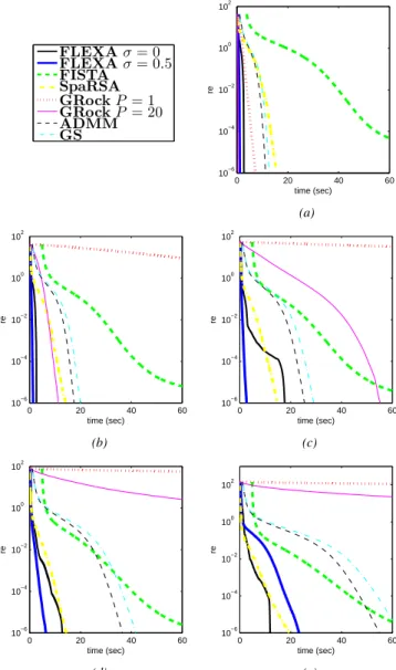
Numerical Tests: We generated six groups of LASSO problems using the random generation technique proposed by Nesterov [10]; this method permits to control the sparsity of the solution. For the first five groups, we considered problems with 10,000 variables and matrix A having 9,000 rows. The five groups differ from the degree of sparsity of the solution; more specifically the percentage of non zeros in the solution is 1%, 10%, 20%, 30%, and 40%, respectively. The last group is formed by instances with 100,000 variables and 5000 rows for A, and solutions having 1% of non zero variables. In all experiments and for all the algorithms, the initial point was set to the zero vector.
Results of our experiments for each of the 10,000 variables groups are reported in Fig. 1, where we plot the relative error as defined in (10) versus the CPU time; all the curves are averaged over ten independent random realizations. Note that the CPU time includes communication times (for distributed algorithms) and the initial time needed by the methods to perform all pre-iterations computations (this explains why the curves associated with FISTA start after the others; in fact FISTA requires some nontrivial initializations based on the computation of ∥A∥22).
Results of our experiments for the LASSO instance with 100,000 variables are reported in Fig. 2. The curves are averaged over three random realizations. Note that we have not included the curves for sequential algorithms (ADMM and GS) on this group of big problems, since we could not use the same nodes used to run all the other algorithms, due to mem-ory limitations. However, we tested ADMM and GS on these big problems on different high-memory nodes; the obtained results (not reported here) showed that, as the dimensions of the problem increase, sequential methods perform poorly in comparison with parallel methods; therefore we excluded ADMM and GS in the tests for the LASSO instance with 100,000 variables.
Given Fig. 1 and 2, the following comments are in order. On all the tested problems, FLEXA withσ= 0.5outperforms in a consistent manner all other implemented algorithms. Results for FLEXA with σ = 0 are quite similar to those with σ= 0.5on the 10,000 variables problems. However on larger problems FLEXAσ= 0(i.e., the version wherein all variables
FLEXAσ= 0 FLEXAσ= 0.5 FISTA SpaRSA GRockP = 1 GRockP = 20 ADMM GS 0 20 40 60 10−6 10−4 10−2 100 102 time (sec) re (a) 0 20 40 60 10−6 10−4 10−2 100 102 time (sec) re (b) 0 20 40 60 10−6 10−4 10−2 100 102 time (sec) re (c) 0 20 40 60 10−6 10−4 10−2 100 102 time (sec) re (d) 0 20 40 60 10−6 10−4 10−2 100 102 time (sec) re (e)
Fig. 1: Relative error vs. time (in seconds) for Lasso with 10,000 variables: (a) 1% non zeros - (b) 10% non zeros - (c) 20% non zeros - (d) 30% non zeros - (e) 40% non zeros
0 200 400 600 800 1000 10−6 10−4 10−2 100 time (sec) re FLEXAσ= 0 FLEXAσ= 0.5 FISTA SpaRSA GRockP= 1 GRockP= 20
Fig. 2: Relative error vs. time (in seconds) for Lasso with 100,000 variables
are updated at each iteration) seems ineffective. This result might seem surprising at first sight: why, once all the optimal solutionsxbi(xk, τi)are computed, is it more convenient not to
use all of them but update instead only a subset of variables? We briefly discuss this complex issue next.
Algorithm 1 has the remarkable capability to identify those variables that will be zero at a solution; because of lack of space, we do not provide here the proof of this statement but only an informal description. Roughly speaking, it can be shown that, for k large enough, those variables that are zero in bx(xk,τ) will be zero also in a limiting solution
¯
x. Therefore, suppose that k is large enough so that this identification property already takes place (we will say that “we are in the identification phase") and consider an index i such thatx¯i= 0. Then, ifxki is zero, it is clear, by Steps 3 and
4, that xki′ will be zero for all indicesk′ > k, independently of whetheribelongs toSkor not. In other words, if a variable that is zero at the solution is already zero when the algorithms enters the identification phase,that variable will be zero in all subsequent iterations; this fact, intuitively, should enhance the convergence speed of the algorithm. Conversely, if when we enter the identification phase xk
i is not zero, the algorithm
will have to bring it back to zero iteratively. It should then be clear why updating only variables that we have “strong” reason to believe will be non zero at a solution is a better strategy than updating them all. Of course, there may be a problem dependence and the best value ofσcan vary from problem to problem. But we believe that the explanation outlined above gives firm theoretical ground to the idea that it might be wise to “waste" some calculations and perform only a partial update
of the variables. □
Referring to sequential methods (ADMM and GS), they behave strikingly well on the 10,000 variables problems, if one keeps in mind that they only use one process. However, as already observed, they cannot compete with parallel methods on larger problems. FISTA is capable to approach relatively fast low accuracy solutions, but has difficulties in reaching high accuracy. The version of GRock with P = 20 is the closest match to FLEXA, but only when the problems are very sparse. This is consistent with the fact that its convergence properties are at stake when the problems are quite dense. Furthermore, it should be clear that if the problem is very large, updating only 20 variables at each iteration, as GRock does, could slow down the convergence, especially when the optimal solution is not very sparse. From this point of view, the strategy used by FLEXAσ= 0.5 seems to strike a good balance between not updating variables that are probably zero at the optimum and nevertheless update a sizeable amount of variables when needed in order to enhance convergence. Finally, SpaRSA seems to be very insensitive to the degree of sparsity of the solution; it is comparable to our FLEXA on 10,000 variables problems, but is much less effective on very large-scale problems. In conclusion, Fig. 1 and Fig. 2 show that while there is no algorithm in the literature performing equally well on all the simulated (large and very large-scale) problems, the proposed FLEXA is consistently the “winner”.
B. Logistic regression problems
The logistic regression problem is described in Example #3 (cf. Section III). For such a problem, we implemented the instance of Algorithm 1 described in the same example. More specifically, the algorithm is essentially the same described for LASSO, but with the following differences:
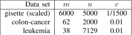
Data set m n c
gisette (scaled) 6000 5000 1/1500 colon-cancer 62 2000 0.01
leukemia 38 7129 0.01
TABLE I: Test problems for logistic regression tests
(a) The approximant Pi is chosen as the second order
ap-proximation of the original functionF;
(b) The initialτiare set to tr(YTY)/2nfor alli, wherenis
the total number of variables andY= [y1y2 · · ·ym]T.
(c) Since the optimal valueV∗ is not known for the logistic regression problem, we no longer use re(x) as merit function but∥Z(x)∥∞, with
Z(x) =∇F(x)−Π[−c,c]n(∇F(x)−x). Here the projection Π[−c,c]n(z) can be efficiently com-puted; it acts component-wise on z, since [−c, c]n =
[−c, c]×· · ·×[−c, c]. Note thatZ(x)is a valid optimality
measure function; indeed,Z(x) = 0is equivalent to the standard necessary optimality condition for Problem (1), see [6]. Therefore, whenever re(x) was used for the Lasso problems, we now use∥Z(x)∥∞ [including in the step-size rule (11)].
We simulated three instances of the logistic regression problem, whose essential data features are given in Table I; we downloaded the data from the LIBSVM repository http://www.csie.ntu.edu.tw/∼cjlin/libsvm/, which we refer to for a detailed description of the test problems. In our implementation, the matrix Y is stored in a column block distributed manner Y = [Y1Y2· · · YP],
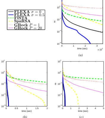
whereP is the number of parallel processors. We compared FLEXA σ = 0and FLEXA σ = 0.5 with the other parallel algorithms, namely: FISTA, SpaRSA, and GRock. We do not report results for the sequential methods (GS and ADMM) because we already ascertained that they are not competitive. The tuning of the free parameters in all the algorithms is the same as in Fig. 1 and Fig. 2.
In Fig. 3 we plotted the relative error vs. the CPU time (the latter defined as in Fig. 1 and Fig. 2). Note that this time in order to plot the relative error, we had to preliminary estimate V∗ (which we recall is not known for logistic regression problems). In order to do so we ran FLEXA with σ = 0.5 until the merit function value∥Z(xk)∥
∞ went below 1e−6, and used the corresponding value of the objective function as estimate of V∗. We remark that we used this value only to plot the curves in Fig. 3.
Results on Logistic Regression reinforce the conclusion we made based on the experiments on LASSO problems. Actually, Fig. 3 clearly shows that on these problems both FLEXA methods significantly and consistently outperform all other solution methods.
In conclusion, our experiments indicate that our algorithmic framework can lead to very efficient and practical solution methods for large-scale problems, with the flexibility to adapt to many different problem characteristics.
FLEXAσ= 0 FLEXAσ= 0.5 FISTA SpaRSA GRockP= 1 GRockP= 20 0 1 2 3 x 10⁴ 10−6 10−4 10−2 100 time (sec) re (a) 0 0.5 1 1.5 2 10−6 10−4 10−2 100 102 time (sec) re (b) 0 1 2 3 4 5 10−6 10−4 10−2 100 102 time (sec) re (c)
Fig. 3: Relative error vs. time (in seconds) for Logistic Regression: (a) gisette - (b) colon-cancer - (c) leukemia
VII. CONCLUSIONS
We proposed a highly parallelizable algorithmic scheme for the minimization of the sum of a possibly noncovex differentiable function and a possibily nonsmooth but block-separable convex one. Quite remarkably, our framework leads to different (new) algorithms whose degree of parallelism can be chosen by the user, ranging from fully parallel to sequential schemes, all of them converging under the same conditions. Many well know sequential and simultaneous solution methods in the literature are just special cases of our algorithmic framework. Our preliminary tests are very promis-ing, showing that our algorithms consistently outperform state-of-the-art schemes. Experiments on larger and more varied classes of problems (including those listed in Section II) are the subject of our current research. We also plan to investigate asynchronous versions of Algorithm 1, the latter being a very important issue in many distributed settings.
APPENDIX
We first introduce some preliminary results instrumental to prove both Theorem 1 and Theorem 2. Hereafter, for notational simplicity, we will omit the dependence of bx(y,τ)onτ and write bx(y). Given S ⊆ N and x ≜ (xi)Ni=1, we will also
denote by (x)S (or interchangeably xS) the vector whose
component iis equal to xi ifi∈S, and zero otherwise.
A. Intermediate results
Lemma 4: LetH(x;y)≜∑ihi(xi;y). Then, the
follow-ing hold:
(i) H(•;y)is uniformly strongly convex onX with constant cτ >0, i.e.,
(x−w)T(∇xH(x;y)− ∇xH(w;y))≥cτ∥x−w∥ 2 ,
(12) for allx,w∈X and given y∈X;
(ii) ∇xH(x;•)is uniformly Lipschitz continuous on X, i.e., there exists a0< L∇H <∞independent onx such that
∥∇xH(x;y)− ∇xH(x;w)∥ ≤ L∇H ∥y−w∥, (13)
for ally,w∈X and given x∈X.
Proof:The proof is standard and thus is omitted.
Proposition 5: Consider Problem (1) under A1-A6. Then the mappingX ∋y7→xb(y)has the following properties: (a) xb(•) is Lipschitz continuous on X, i.e., there exists a positive constantLˆ such that
∥xb(y)−xb(z)∥ ≤ Lˆ ∥y−z∥, ∀y,z∈X; (14)
(b) the set of the fixed-points of xb(•)coincides with the set of stationary solutions of Problem (1); therefore bx(•) has a fixed-point;
(c) for every given y ∈X and for any setS ⊆ N, it holds that (bx(y)−y)TS ∇xF(y)S+ ∑ i∈S gi(bxi(y))− ∑ i∈S gi(yi) (15) ≤ −cτ ∥(xb(y)−y)S∥ 2 , withcτ ≜qminiτi.
Proof: We prove the proposition in the following order: (c), (a), (b).
(c): Given y ∈ X, by definition, each bxi(y) is the unique
solution of problem (3); then it is not difficult to see that the following holds: for all zi∈Xi,
(zi−bxi(y)) T
∇xihi(xbi(y);y) +gi(zi)−gi(bxi(y))≥0. (16) Summing and subtracting ∇xiPi(yi;y) in (16), choosing
zi=yi, and using P2, we get
(yi−bxi(y)) T (∇xiPi(bxi(y);y)− ∇xiPi(yi;y)) + (yi−bxi(y)) T ∇xiF(y) +gi(yi)−gi(xbi(y)) −τi(bxi(y)−yi)TQi(y) (bxi(y)−yi)≥0, (17)
for alli∈ N. Observing that the term on the first line of (17) is non positive and using P1, we obtain
(yi−bxi(y)) T ∇xiF(y) +gi(yi)−gi(xbi(y)) ≥cτ∥bxi(y)−yi∥ 2 ,
for alli∈ N. Summing overi∈S we get (15).
(a): We use the notation introduced in Lemma 4. Giveny,z∈
X, by optimality and (16), we have, for allv andw inX (v−bx(y))T∇xH(bx(y);y) +G(v)−G(bx(y))≥0 (w−xb(z))T∇xH(bx(z);z) +G(w)−G(xb(z))≥0. Setting v=bx(z)andw =bx(y), summing the two inequal-ities above, and adding and subtracting ∇xH(xb(y);z), we