Sensor placement for leak detection and
location in water distribution networks
R. Sarrate*, J. Blesa, F. Nejjari, J. Quevedo
Automatic Control Department, Universitat Politècnica de Catalunya, Rambla de Sant Nebridi, 10, 0222 Terrassa, Spain
*Corresponding author, e-mail [email protected]
ABSTRACT
The performance of a leak detection and location algorithm depends on the set of measurements that are available in the network. This work presents an optimization strategy that maximizes the leak diagnosability performance of the network. The goal is to characterize and determine a sensor configuration that guarantees a maximum degree of diagnosability while the sensor configuration cost satisfies a budgetary constraint. To efficiently handle the complexity of the distribution network an efficient branch and bound search strategy based on a structural model is used. However, in order to reduce even more the size and the complexity of the problem the present work proposes to combine this methodology with clustering techniques. The strategy developed in this work is successfully applied to determine the optimal set of pressure sensors that should be installed to a District Metered Area in the Barcelona Water Distribution Network.
KEYWORDS:
Leak detection and location, sensor placement, structural analysis, waterdistribution network
1.
INTRODUCTION
An important matter concerning water distribution networks is system water loss, which has a meaningful effect on both water resource savings and costs of operation (Farley and Trow, 2003). Continuous improvements on water loss management are being applied. New technologies are developed to achieve higher levels of efficiency, intended to reduce losses to acceptable levels considering technical and economical aspects. Usually a leakage detection method in a District Metered Area (DMA) starts analyzing input flow data, such as minimum night flows and consumer metering data. Once the water distribution district is identified to have a leakage, techniques are used to locate the leakage for pipe replacement or repairing. The whole process could take weeks or months with an important volume of water wasted. To overcome this problem, different leakage detection and location techniques are carried out in the field. Fault diagnosis techniques are applied by Brdys and Ulanicki (1994). A mathematical model is used which permits comparing the data gathered by installed sensors in the network with the data obtained by a model of this network. If a difference is detected between these data sets, a detection of an abnormal event is obtained. Thus, modeling is paramount in order to achieve successful results. This model is the mathematical tool linking the real sensor data gathered from the network to the decision making procedure. The tool provides leak detection as well as its approximate location in the network.
Fault diagnosis systems are an increasing and important topic in many industrial processes. The number of publications devoted to fault diagnosis has increased notably in the last years (Blanke et al., 2006). In model-based fault diagnosis, diagnosis is basically performed based on the responses of residual generators. These are functions obtained from the model which perform the task of comparing the process model and on-line process information. Since process information is usually obtained by means of the sensors installed in the process, it is important to develop methodologies to place the correct sensor set in the process in order to guarantee some diagnosis specifications.
Some results devoted to sensor placement for diagnosis can be found in (Travé-Massuyès et al., 2006; Krysander and Frisk, 2008; Sarrate et al., 2012). All these works use a structural model-based approach and define different diagnosis specifications to solve the sensor placement problem. A structural model is a coarse model description, based on a bi-partite graph, which can be obtained early in the development process, without major engineering efforts. This kind of model is suitable to handle large scale systems since efficient graph-based tools can be used and does not have numerical problems. Structural analysis is a powerful tool for early determination of fault diagnosis performances (Blanke et al., 2006). In (Sarrate et al., 2012) an algorithm is developed to determine where to install a specific number of pressure sensors in a DMA in order to maximize the capability of detecting and isolating leaks. The number of sensors to install is limited in order to satisfy a budgetary constraint requirement. Despite an efficient branch and bound search strategy based on a structural model is used, its applicability is still limited to medium-sized networks. In order to overcome this drawback by reducing even more the size and the complexity of the problem the present work proposes to combine this methodology with clustering techniques. Clustering is the unsupervised classification of patterns (observations, data items, or feature vectors) into groups (clusters). The clustering problem has been addressed in many contexts and by researchers in many disciplines (Jain et al., 1999). It is a mature and active research area (Xu and Wunsch, 2005) and many efficient algorithms have been developed in the literature.
The main contribution of this paper consists in combining a clustering technique with a branch and bound search based on a structural model to solve the sensor placement problem. This methodology is applied to a DMA network in Barcelona to determine the best location of pressure sensors for leak detection and location.
This paper is organized as follows. In Section 2, some model-based fault diagnosis concepts are reviewed. Section 3 formally states the sensor placement problem. In Section 4 the structural approach to sensor placement is recalled, whereas the clustering approach is described in Section 5. Next, the whole methodology is applied to a DMA network in Section 6. Finally some conclusions are given in Section 7.
2.
MODEL-BASED FAULT DIAGNOSIS
Model-based fault diagnosis is a consolidated research area (Blanke et al., 2006). Most approaches to detect and isolate faults are based on consistency checking. The basic idea behind all these works is the comparison between the observed behavior of the process and its corresponding model. This is performed by means of consistency relations, which can be roughly described as a function of the form
where ( )y t and ( )u t are vectors of known variables, denoting respectively process measurements and process control inputs. Function h is obtained from the model and is the basis to generate a residual
( ) ( ( ), ( ))
r t h y t u t . (2)
A residual is a temporal signal indicating how close is behaving the process compared with its expected behavior predicted by the model. At the absence of faults, a residual equals zero. In fact, a threshold based test is usually implemented in order to cope with noise and model uncertainty effects. Otherwise, when a fault is present the model is no longer consistent with the observations (known process variables) and the residual exceeds the prefixed threshold. Detecting faults is possible with only one residual sensitive to all faults. However, fault isolation is usually required rather than just detecting the presence of a fault. The fault isolation task is performed by designing a set of residuals based on several consistency relations. Each residual is sensitive to different faults such that the residual fault signature is unique for each fault. Therefore, distinguishing the actual fault from other faults is possible by looking at the residual fault signature. These fault signatures are usually collected in matrix form.
Given a set of residuals R and a set of faults F the fault sensitivity matrix is defined in (3).
When an element ij is close to zero then residual riR is weakly sensitive to fault fjF, whereas when it diverges from zero then the residual is strongly sensitive to the
fault fj. 1 1 · · 1 m n n 1 m r r f f r r f f (3)
This matrix can be obtained by convenient model equations manipulation as long as faults effects are included in them (Blesa et al., 2012). Alternatively, it can be obtained by sensitivity analysis through simulation (Pérez et al., 2011). The latter approach will be used in the present paper. Given a set of possible measurable variables
x x1, , ,2xn
, the fault sensitivity matrix will collect those (primary) residuals that are obtained by comparing each real measurement xi to the corresponding signal obtained through simulation ˆxi in the fault free case, i.e. ri xi xˆi. An approximate procedure to obtain the fault sensitivity matrix involves using a simulator to get an estimation of measurement xi in the fault free casexˆi0, aswell as in every faulty situation ˆ ,xij fj F, i.e. ij xˆijxˆi0.
Sometimes a binary version of the fault sensitivity matrix is used. Then the corresponding binary residuals are usually called structured residuals, whereas in the non-binary matrix they are referred to as directional residuals.
3.
PROBLEM FORMULATION
Let S be the candidate sensor set and m the number of sensors that will be installed in the
system. Then, the problem can be roughly stated as the choice of a combination of m sensors in S such that the diagnosis performance is maximized. It is assumed that a bounded budget is
assigned to instrumentation and that all sensors to be installed have equal cost. This is the case in the DMA application, since all candidate sensors will be pressure sensors.
Let F be the set of faults that must be monitored. In a water distribution domain a leak is an
example of a fault, but other damages could be considered such as pipe blocking or tank overflow. In this work, the single fault assumption will hold (i.e., multiple faults will not be covered) and no candidate sensor fault will be considered. In model-based diagnosis, fault detectability and fault isolability are the main objectives (Blanke et al., 2006). Assuming structured residuals, a fault is detectable if its occurrence can be monitored, whereas a fault
i
f F is isolable from a fault fjF if the occurrence of fi can be detected independently of the occurrence of fj.
Assuming that a sensor configuration SS is installed in the process, F SD( )F will denote
the detectable fault set. Fault isolability will be characterized by means of fault pairs. Let:FF be all fault pairs, then ( )F SI will denote the set of isolable fault pairs (i.e., ( , )f fi j F SI( ) means that fault fi is isolable from fj when the sensor configuration S is installed in the system). Based on the set of isolable fault pairs the isolability index is defined as the number of isolable fault pairs when a sensor configuration S is installed, i.e. I(S)=|FI(S)|, where |·| denotes the cardinality of the set.
To solve the sensor placement problem proposed in this paper, a system description is also required. Such description will allow the computation of the detectable faults and the isolability index for a given sensor configuration. Hence, the sensor placement for fault diagnosis can be formally stated as follows:
GIVEN a candidate sensor set S, a system description , a fault set F, and the
number m of sensors to be installed.
FIND the m-sensor configuration SS such that F SD( )Fand
( ) ( ), | |
I S I S S S S m.
This problem was already solved in (Sarrate et al., 2012), using a branch and bound search strategy based on a structural model of the process. However, the complexity of such algorithm critically depends on the cardinality of S. In order to overcome this constraint, a
preprocessing step is proposed in the present paper. Clustering techniques will be applied to reduce the candidate sensor set before solving the sensor placement problem as in (Sarrate et al., 2012).
4.
STRUCTURAL APPROACH TO SENSOR PLACEMENT
4.1Fault diagnosis based on structural analysisThe analysis of the model structure has been widely used in the area of model-based fault diagnosis (Blanke et al., 2006). Therefore, consistent tools exist in order to perform diagnosability analysis and consequently compute the set of detectable and isolable faults. The structural model is often defined as a bipartite graph ( , , )G M X A where M is a set of model equations, X a set of unknown variables and A a set of edges, such that ( , )e xi j Aas long as equation eiM depends on variablexjX . A structural model is a graph representation of the analytical model structure since only the relation between variables and equations is taken into account, neglecting the mathematical expression of this relation.
Structural modeling is suitable for an early stage of the system design, when the precise model parameters are not known yet, but it is possible to determine which variables are related to each equation. Furthermore, the diagnosis analysis based on structural models is performed by means of graph-based methods which have no numerical problems and are more efficient, in general, than analytical methods. However, due to its simple description, it cannot be ensured that the diagnosis performance obtained from structural models will hold for the real system. Thus, only best case results can be computed.
It is well-known that the over-determined part of the model is the only useful part for system monitoring (Blanke et al., 2006). The Dulmage-Mendelsohn decomposition (Dulmage and Mendelsohn, 1958) is a bipartite graph decomposition that defines a partition on the set of model equations M. It turns out that one of these parts is the over-determined part of the model and is represented as M+.
Fault detectability and isolability can be defined as properties of the over-determined part of the model (Krysander and Frisk, 2008). First, it is assumed that a single fault f F can only
violate one equation (known as fault equation), denoted byef M. Without loss of generality, it is assumed also that a sensor sS can only measure one single unknown
variablexsX . In the structural framework, such sensor will be represented by one single equation (known as sensor equation), denoted as es. Given a set of sensors S, the set of sensor equations is denoted asMS. Thus, given a candidate sensor configuration S and a model M, the updated system model corresponds toMSM . Hence, the dectectable fault set and the set of isolable fault pairs can be determined as
( ) F | D f S F S f e M M , (4)
( ) , | \ i j I i j f S f F S f f e M M e . (5)4.2Optimal sensor placement algorithm
The sensor placement algorithm developed in (Sarrate et al., 2012) is briefly recalled in this section. Algorithm 1 is based on a depth-first branch and bound search. The search involves building a node tree by recursively calling function searchOpm, beginning at the root node down to the leaf nodes. Each node corresponds to a sensor configuration (node.S) and child
nodes are built by removing sensors from its corresponding parent node. Set node.R specifies those sensors that are allowed to be removed.
Algorithm 1 S* = searchOpm(node, S*) childNode.R := node.R
for m-(|S|-|R|)+1 iterations do
Takes childNode.R at random childNode.S := node.S\
s childNode.R := childNode.R\
sif I(childNode.S) > I(S*) and FD(childNode.S) = F then
if |childNode.S| > m then S* := searchOpm(childNode, S*) else S* := childNode.S if I(node.S)=I(S*) then return S* end if end if end if end for return S*
Throughout the search, the best solution is updated in S* whenever an m-sensor configuration with a higher fault isolability index than the current best one is found, given that all faults are detectable. The search is initialized as follows: node.S = node.R = S and S* = Ø. During the
search only those branches that can be further expanded to an m-sensor configuration are visited. Tree expansion is aborted whenever the fault isolability index is not improved or some faults are not detectable.
5.
CLUSTERING APPROACH TO SENSOR PLACEMENT
5.1Clustering techniques
Given a set of elements
x x1, , ,2 xn
, clustering consists in partitioning the n observationsinto l sets
1, 2, , l
(l ≤ n) in such a way that objects in the same group (called cluster) are more similar (in some sense) to each other than those in other groups (clusters). For example, k-means clustering algorithm (MacQueen, 1967) minimizes the within-cluster sum of distances by solving the optimization problem
1 arg min , j i l j i i d
x x , (6)where d is a distance and i is the centroid of cluster i (i.e. it is the mean of observations in i
according to metric d). In the original algorithm, d is the squared Euclidean distance, but other distance measures are possible. Problem (6) is nonconvex and obtaining the solution is NP-hard, but there are efficient heuristic algorithms that converge quickly to a local optimum.
5.2Problem reduction through clustering techniques
In this paper, we propose a reduction in the number of candidate sensors by grouping the n initial sensors into l groups (l ≤ n) applying the k-means algorithm. Then, a representative sensor will be selected for each cluster, setting up the new candidate sensor set.
In this case, the criterion used for determining the similitude between elements (sensors) is the sensitivity pattern of their primary residuals to faults. In particular, according to the procedure described in Section 2, this is given by every row i of the fault sensitivity matrix defined in (3). So, choosing xj=j, j1,...,n(wherejis the j row vector of matrix) and applying the k-means algorithm defined in (6), a set of l clusters of sensors with a similar fault sensitivity pattern will be obtained. Since residuals are directional, the cosine distance is chosen for the k-means algorithm.
Once the elements xj (sensors) have been grouped in l clusters, the most representative sensors ci, i=1, …, l can be chosen as the nearest ones to the cluster centroids among the elements of each cluster.
6.
APPLICATION TO A WATER DISTRIBUTION NETWORK
6.1Water network description
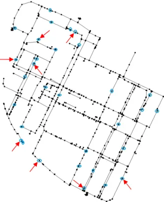
The sensor placement methodology is applied to a DMA located in Barcelona area (see Figure 2). It has 883 nodes and 927 pipes. The network consists of 311 nodes with demand (RM type), 60 terminal nodes with no demand (EC type), 48 hydrant nodes without demand (HI type), 14 dummy valve nodes without demand (VT type) and 448 dummy nodes without demand (XX type). The network has two inflow inputs modeled as reservoir nodes.
Leakage detection is based on the premise that damage (leakage) in one or more locations of the piping network involves local liquid outflow at the leakage location, which will change the flow characteristics (pressure heads, flow rates, acoustics signals, etc.) at the monitoring locations of the piping network. In this work, it is assumed that leaks might only occur at XX type nodes, so there are 448 potential leaks to be detected and located. Actually leaks could occur at any network node or pipe. However, leak locations have been restricted to certain type nodes in order to delimit the size and complexity of the problem.
A similar practical reason applies when defining the possible location of the network monitoring points. Pressure sensors at RM type nodes will be used as network monitoring points, so there are 311 candidate sensors that could be chosen for installation. Despite measuring flow rate could also be useful for leak detection, collecting pressure data is cheaper and easier, and pressure transducers give instantaneous readings whereas most flow meters do not react instantaneously to flow changes (de Schaetzen et al., 2000).
6.2Water network model
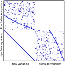
Solving the sensor placement problem defined in Section 3 requires a structural model of the water network (as described in Section 4.1) and a fault sensitivity matrix (see Equation (3)). The model of the DMA comprises 883 flow balance equations
i n i n q Q q d
, (7)where Qn represents all flows corresponding to incident edges to node n and dn is the known flow demand of node n, and 927 pipe flow equations
( ) ( )
e e
q t f p , (8)
where qe is the flow corresponding to edge e and f is a nonlinear function of the pressure drop on the adjacent nodes of edge e. These equations depend on 927 unknown flow variables and 883 unknown pressure variables. The resulting structural model is depicted in Figure 1. A dot (i, j) in the figure indicates that variable i appears in equation j.
fl ow ba lanc e eq ua ti on s p ip e f lo w eq uat io ns
flow variables pressure variables
Figure 1. Structural DMA model.
A leak in a node involves violating a flow balance equation, so fault equations are Equation (7) for type XX nodes.
A fault sensitivity matrix has been also obtained using the EPANET hydraulic simulator. Given a set of boundary conditions (such as water demands) EPANET software has been firstly used to estimate the steady-state pressure at the 311 RM type nodes. Next, 448 leaks have been simulated in the XX type nodes and the steady-state pressure has been estimated again in the 311 RM type nodes. Finally, a 311 448 fault sensitivity matrix has been obtained as the pressure difference between the fault free case and each faulty situation, according to the procedure described in Section 2. Although the fault sensitivity matrix depends on the leakage size, the diagnosability properties are robust against this uncertainty. So in this work the minimum detectable leakage size has been considered in the simulations.
6.3Sensor placement analysis and results
In principle, to fully isolate all 448 possible leaks, the required isolability index should be
448
2 100128
. However, according to the structural analysis, installing all 311 candidate sensors, the isolability index would just be 100099. Achieving a better performance would require installing more sensors than those designated in the candidate sensor set. Therefore, there is a trade-off between the diagnosis performance and the number of installed sensors. Assume that the water distribution company has established a maximum budget for investment on instrumentation that makes it possible to install up to 8 pressure sensors. Hence, the water distribution company wants to install 8 sensors maximizing the resulting
since it would require a huge amount of computation time. So first of all the candidate sensor set will be reduced by applying the clustering approach described in Section 5.2.
k-means algorithm has been applied to partition the initial candidate sensor set into 31 clusters, and a representative sensor for each cluster has been found. So, the new candidate sensor set has now 31 pressure sensors (see the blue circled nodes in Figure 2). Next, applying Algorithm 1 the 8-sensor configuration, pointed by a red arrow in Figure 2, is obtained. With these 8 sensors all leaks can be detected and the isolability index amounts to 100092.
Figure 2. DMA network sensor placement results.
Regarding performance issues the clustering step takes around 22 s, whereas the branch and bound search takes more than 7 h. Bearing in mind this computation time difference, it might sound appealing to directly apply the clustering step to obtain the 8-sensor configuration. However, this would not necessarily produce the same results for several reasons. First, it is well known that although the k-means algorithm finds an optimum partition, it does not necessarily find the global one. In fact, the algorithm is significantly sensitive to the initial randomly selected cluster centres. To alleviate this drawback the algorithm is commonly run multiple times with different initial conditions. Secondly, notice that only a reduced set of directional residuals (the primary residuals) are represented in the fault sensitivity matrix according to the simulation method proposed in (Pérez et al., 2011). In fact, the full set of directional residuals that could be designed based on the model equations would be much bigger, but computationally harder to obtain. The structural analysis approach takes all structured residuals into account, instead. Thus its results are more complete. Therefore, the sole purpose of the clustering step is complexity reduction. But the branch and bound step is always desirable since it produces sound and complete results.
Despite the branch and bound search is time consuming, its performance is much better than that of an exhaustive search. Remark that during the branch and bound search, the most demanding operation is evaluating the isolability index through Equation (5), which takes in average 1.24 s in this case. Whereas Algorithm 1 just computes it 17286 times, an exhaustive
search would involve evaluating it
8
7888725
times, which would require more than 100 days.
CONCLUSIONS
This work presents an optimal sensor placement strategy that maximizes the water network leak diagnosability. The goal is to characterize and determine a sensor set that guarantees a maximum degree of diagnosability while a budgetary constraint is satisfied. To overcome the complexity of the problem this work proposes the combination of a branch and bound search based on a structural model of the distribution network and clustering techniques. The strategy developed is successfully applied to a District Metered Area of the Barcelona Water Distribution Network. The results show that this combined technique manages to solve the sensor placement problem in a reasonable time, which otherwise would not be possible. Although promising, these are preliminary results and more research has to be done. One the one hand, as already mentioned in Section 6.3, the k-means algorithm does not guarantee a global optimal solution so the performance of other clustering techniques should be investigated. On the other hand, applying clustering techniques to reduce the problem complexity by partitioning the fault set could be investigated.
ACKNOWLEDGEMENTS
This work has been funded by the Spanish MINECO through the project CYCYT SHERECS (ref. DPI2011-26243), and by the European Commission through contracts i-Sense (ref. FP7-ICT-2009-6-270428) and EFFINET (ref. FP7-ICT2011-8-318556).
REFERENCES
Blanke M., Kinnaert M., Lunze J. and Staroswiecki M. (2006). Diagnosis and Fault-Tolerant Control. Springer, 2nd ed.
Blesa J., Puig V. and Saludes J. (2012). Robust identification and fault diagnosis based on uncertain multiple input–multiple output linear parameter varying parity equations and zonotopes. J. Proc. Cont., 22(10), 1890–1912.
Brdys M.A. and Ulanicki B. (1994). Operational Control of Water Systems: Structures, Algorithms, and Applications. Prentice Hall International.
Dulmage A.L. and Mendelsohn N.S. (1958). Coverings of bipartite graphs. Canad. J. Math., 10, 517–534. Farley M. and Trow S. (2003). Losses in Water Distribution Networks. IWA Publishing.
Jain A.K., Murty M.N. and Flynn P.J. (1999). Data clustering: a review. ACM Comput. Surv., 31(3), 264–323. Krysander M. and Frisk E. (2008). Sensor placement for fault diagnosis. IEEE Trans. Syst. Man Cybern. A,
38(6), 1398–1410.
MacQueen J. (1967): Some methods for classification and analysis of multivariate observations. In: Proc. 5th Berkeley Symp. on Math. Statist. and Prob., Berkeley, 1, 281–297. Univ. of Calif. Press.
Pérez R., Puig V., Pascual J., Quevedo J., Landeros E. and Peralta A. (2011). Methodology for leakage isolation using pressure sensitivity analysis in water distribution networks. Contr. Eng. Pract., 19(10), 1157– 1167.
Sarrate R., Nejjari F. and Rosich A. (2012): Sensor placement for fault diagnosis performance maximization in distribution networks. In: Proc. 20th Medit. Conf. on Cont. & Autom., Barcelona, Spain, 110–115, July 2012.
de Schaetzen W.B.F., Walters G.A. and Savic D.A. (2000). Optimal sampling design for model calibration using shortest path, genetic and entropy algorithms. Urb. Wat., 2(2), 141–152.
Travé-Massuyès L., Escobet T. and Olive X. (2006). Diagnosability analysis based on component-supported analytical redundancy relations. IEEE Trans. Syst. Man Cybern. A, 36(6), 1146–1160.