arXiv:1806.03582v3 [cs.AI] 27 Feb 2019
A Scalable Framework for Trajectory Prediction
Punit Rathore, Dheeraj Kumar, Sutharshan Rajasegarar, Marimuthu Palaniswami,
Fellow, IEEE
, James. C.
Bezdek,
Life Fellow, IEEE
Abstract—Trajectory prediction (TP) is of great importance for a wide range of location-based applications in intelligent transport systems such as location-based advertising, route plan-ning, traffic management, and early warning systems. In the last few years, the widespread use of GPS navigation systems and wireless communication technology enabled vehicles has resulted in huge volumes of trajectory data. The task of utilizing this data employing spatio-temporal techniques for trajectory prediction in an efficient and accurate manner is an ongoing research problem. Existing TP approaches are limited to short-term predictions. Moreover, they cannot handle a large volume of trajectory data for long-term prediction. To address these limitations, we propose a scalable clustering and Markov chain based hybrid framework, called Traj-clusiVAT-based TP, for both short-term and long-term trajectory prediction, which can handle a large number of overlapping trajectories in a dense road network. Traj-clusiVAT can also determine the number of clusters, which represent different movement behaviours in input trajectory data. In our experiments, we compare our proposed approach with a mixed Markov model (MMM)-based scheme, and a trajectory clustering, NETSCAN-based TP method for both short- and long-term trajectory predictions. We performed our experiments on two real, vehicle trajectory datasets, including a large-scale trajectory dataset consisting of3.28million trajectories obtained from 15,061 taxis in Singapore over a period of one month. Experimental results on two real trajectory datasets show that our proposed approach outperforms the existing approaches in terms of both short- and long-term prediction performances, based on prediction accuracy and distance error (in km).
Index Terms—Large-scale trajectory data, next location pre-diction, Long-term trajectory prepre-diction, scalable clustering.
I. INTRODUCTION
With the widespread use of Global Positioning System
(GPS) devices, smart-phones, Internet of Things [1], and wireless communication technology, it is possible to track all kinds of moving objects all over the world. The increasing prevalence of location-acquisition technologies has resulted in large volumes of spatio-temporal data, especially in the form of trajectories. These data often contain a great deal of information [2], which give rise to many location-based services (LBSs) and applications such as vehicle navigation, traffic management, and location-based recommendations. One
Punit Rathore, and Marimuthu Palaniswami are with the Department of Electrical and Electronic Engineering, The University of Melbourne, Parkville, Victoria, Australia.
E-mail: {prathore@student., palani@}unimelb.edu.au.
Dheeraj Kumar is with the Lyles School of Civil Engineering, Purdue University, USA.
E-mail: [email protected]
Sutharshan Rajasegarar is with the School of Information Technology, Deakin University, Geelong, Victoria, Australia.
E-mail: [email protected].
James C. Bezdek is with the School of Computing and Information Systems, The University of Melbourne, Victoria, Australia.
E-mail: [email protected].
key operation in such applications is the route prediction of moving objects.
Vehicle route prediction allows certain services to improve their quality e.g. if the route of vehicles is known in advance,
intelligent transportation systems (ITSs) can provide
route-specific traffic information to drivers such as forecasting traffic conditions and routing the driver so as to avoid traffic jams. Route prediction also enables location-based advertis-ing, which can advertise certain products/services and special offers to the target commuters most likely to pass through business outlets and stores based on their travel trajectory.
With the advancement in artificial intelligence, various machine learning techniques have now been used for trajectory analysis. Recently, several studies have been carried out on
trajectory prediction, particularly after Songet al.[3]
demon-strated a 93% potential for predictability in user mobility, which supplied the theoretical basis for location prediction methods. These methods mainly focus on two kinds of pre-diction models. The first type is the short-term trajectory prediction model, which aims to predict the next-location or a few locations in the near future. These models usually rely on current location and one or two previous locations of an object to predict its next location. The second type is the long-term trajectory prediction model which focuses on location prediction at a more distant future time or on complete route prediction. These models generally rely on an available partial trajectory of a moving object to predict the complete trajectory. In urban areas, vehicle trajectories are usually constrained to a complex road network with many parallel and perpendicular road segments and intersections, which makes their time progression very irregular. Due to the uncertainty of moving objects, most of the existing trajectory prediction methods only focus on predicting short-term partial trajectories. They have poor prediction accuracy for long-term trajectory predictions and they do not work well for estimating continuous and complete trajectories.
The sheer amount of vehicle trajectory data, if analyzed effectively, can significantly improve route prediction per-formance. However, it is challenging to carry out trajectory prediction from a large amount of trajectory data. The huge volumes of data to be processed precludes using machine
learning based traditional prediction (TP) methods. Most of
the existing trajectory prediction schemes cannot handle a large number of trajectories, especially when they span a large area of a road network. Existing TP methods are hybrid in nature and usually employ classical frequent sequential pattern based algorithms, Markov model-based algorithms, or clustering based algorithms to a small amount of training data. Apriori-like sequential pattern methods bear significant com-putational overhead in mining frequent patterns because they
produce a huge number of candidate sequences and require multiple scans of the database. Markov model approaches such as higher-order Markov models incur significant overhead in terms of computation time and space for storing and learning the mobility model. Similarly, parameter learning algorithms in Hidden Markov models impose significant computational burdens for large-scale trajectory datasets. Existing trajectory clustering based location prediction approaches are not scal-able due to distance matrix computations for big data and are not able to handle a large number of overlapping trajectories efficiently. Therefore, most TP methods demonstrated in the literature use synthetic or small to medium size real trajectory datasets. To the best of our knowledge, the largest real dataset was used in [4], consisting of 370 million GPS points. These authors utilized a parallel processing model, MapReduce, in their implementation to handle large datasets.
To address these challenges and overcome the drawbacks of existing TP methods, this paper presents a novel, scalable framework for both short-term and long-term TP, which is suit-able for large numbers of overlapping trajectories in a dense road network, typical for major cities around the world. First, we cluster the large trajectory data using a modified version of our two-stage clusiVAT (clustering using improved Visual Assessment of Tendency) algorithm [5], [6], which we call
Traj-clusiVAT, implemented for trajectory prediction task. The
Traj-clusiVAT algorithm first extracts a smart sample using
the Maximin-Random sampling (MMRS) scheme [7], which
provides a good representation of the input cluster structure
(present in the original data). Then, it uses the improved
visual assessment of cluster tendency (iVAT) algorithm to
visually determine the number of clusters (k) in input data, and
subsequently, it partitions the trajectory sample intokclusters
which contain different frequent movement patterns in the trajectory data. Then, the remaining non-sampled trajectories
are assigned to one of k clusters using thenearest prototype
rule (NPR). Finally, Markov chain models are constructed
from the trajectories in each cluster. These models quantify the movement patterns within clusters, and subsequently, can be used for TP.
Our main contributions in this paper are as follows:
• We propose a novel, hybrid framework for short-term
and long-term trajectory prediction, based on a scalable clustering algorithm and Markov chain model, which can utilize a large number of trajectories in a dense road network.
• We implement a modified version of the two-stage
clusi-VAT algorithm, called as Traj-clusiclusi-VAT, to cluster large numbers of trajectories in an accurate and efficient man-ner. In this regard,
– We develop a new algorithm to compute a
repre-sentative trajectory(RT) for each cluster, and
subse-quently, use it to assign non-sampled trajectories to
one of thekclusters in the nearest prototyping phase.
– We also develop an improved algorithm for nearest
prototyping, which assigns each non-sampled
trajec-tory to one of thekclusters, based on pattern
match-ing and the distance of non-sampled trajectories to
the RT of each cluster.
• We compare our proposed algorithm with two TP
al-gorithms: a mixed Markov model (MMM) [8] and a
trajectory clustering model NETSCAN [9] based algo-rithm. Our experiments used two real-life, taxi trajectory datasets including a large-scale taxi trajectory dataset
consisting of 370 million GPS traces and 3.28 million
passenger trips from 15,061 taxis during the period of
one month in Singapore. To the best of our knowledge, this is the first time TP has been performed on such a large number of real-life road network trajectories. Here is an outline of the rest of this article. Section II discusses related work and limitations. Section III formally defines the problem and presents preliminaries on techniques used in our work. Our novel, hybrid framework, based on Traj-clusiVAT and Markov models, is presented in Section IV, and its time complexity is discussed in Section V. Section VI presents our numerical experiments, including computation protocols, datasets and results, followed by conclusions in Section VII.
II. RELATEDWORK
Several studies address the problem of trajectory predic-tions, which includes the problem of short-term prediction such as predicting the next location, and long-term prediction such as future locations or complete route prediction. These methods mainly focus on discovering frequent patterns using various data mining methods. Many of these methods are hybrid in nature and can be broadly classified into three cate-gories: (i) Rule-based learning based approaches (ii) Markov model-based approaches (iii) Clustering-based approaches.
A. Rule-based learning based approaches
Several rule-based methods have been used for location prediction. Morzy [10] implemented a modified version of the PrefixSpan algorithm to extract association rules from a moving object database, and used frequent pattern tree with a matching function to select the best association rule from
the database of movement rules. Jeunget al. [11] proposed a
hybrid prediction approach, which combines association rules in the form of trajectory patterns with the motion functions of an object’s recent movements, to estimate future locations. Given an object’s recent movement and predictive queries, the best association rule is chosen for prediction. The query processing approaches presented in [11] can only support near and distant-time predictive queries, making them unsuitable for long-term trajectory prediction. Moreover, with the huge number of trajectories, the number of association rules is also huge, which makes association-rule based algorithms impractical for large-scale mobility data.
Monrealeet al. [12] built a decision tree that they called
a T-pattern Tree, based on the frequent movement patterns
extracted using aTrajectory Pattern algorithm, and predicted
the next location of a new trajectory based on the best match-ing functions. However, minmatch-ing of frequent trajectory patterns is computationally expensive. The method in [12] is similar to the use of association rules as predictive rules in rule-based classifiers. Therefore, this method [12] may result in
a large number of predictive rules for voluminous trajectories.
Qiao et al. [13] proposed a TP algorithm, called PrefixTP,
which examines only the prefix subsequences, and projects their corresponding postfix subsequences into projected sets. Then, for a partial trajectory, it recursively finds a postfix sequence based on the minimum support count requirement and then declares the most frequent sequential pattern as the most probable trajectory. Finding subsets of trajectory sequential patterns is a recursive mining process, which is also computationally extensive.
B. Markov model-based approaches
Markov models (MMs) have been widely used to mine
frequent patterns for route prediction problems. Ishikawa et
al. [14] proposed a model to extract mobility statistics, called
the Markov transition probability, which is based on a cell-based organization of target space and a Markov chain model, and employed R-tree spatial indices to compute Markov
tran-sition probabilities. Simmon et al. [15] presented a Hidden
Markov Model(HMM) based probabilistic approach to predict
a driver’s intended route and destination through observations
of the driver’s habits. Asaharaet al.[8] suggested that standard
MM and HMM are not generic enough to encompass all types of movement behaviour. They proposed a variant of Markov
model, called the mixed Markov-chain model (MMM), as an
intermediate model between individual and generic models, for pedestrian movement prediction.
Gambs et al. [16] extended a previously proposed
mo-bility model, named v-Mobility Markov Chain (v-MMC), to
incorporate thevprevious visited locations. They showed that
prediction accuracy increases with v, but increasing vbeyond
two does not compensate for the significant overhead in terms of computation and space for learning and storing the mobility model. They only considered the sequence of the significant locations, instead of all locations, to build higher order MM.
Zhang et al. [17] proposed a group-level mobility modeling method, Gmove, which alternates between two intertwined tasks, user grouping and mobility modeling, and generates an ensemble of HMMs to characterize group-level movement.
Most of the MMs do not consider the discontinuous chain of the hidden states, and therefore, the state retention problem can drastically degrade the accuracy of location prediction system [13]. For the irregular trajectory data, the movement rules cannot be easily represented by Markov models, which may cause loss of continuous location information [13]. More-over, the HMM approaches use the Baum-Welch algorithm for parameter learning and the Viterbi algorithm to find the most likely sequences of hidden states. These algorithms impose a significant computation burden for large-scale trajectory datasets.
Recently, deep learning techniques such as inverse rein-forcement learning (IRL), long short-term memory (LSTM), and recurrent neural networks (RNNs) have been used for modeling vehicle trajectories [18]–[20]. However, some of these studies are still based on first-order Markov assumption to model the routing decisions for heterogeneous destinations, or they are too shallow which makes the modeling pattern varieties suffer from too few parameters.
C. Clustering based approaches
Some researchers have proposed trajectory clustering based route prediction methods, which partition the trajectories into several clusters representing different motion patterns based on the trajectory similarity. Various clustering approaches [21] using different methods and distance measures between tra-jectories have been proposed in the literature. Road network constrained trajectory clustering approaches can be classified into two broad categories. The first type uses the traditional
clustering approaches suchk-means and DBSCAN with
spe-cially designed distance measures [22]–[25] for trajectories. The second category of algorithms [9], [26] cluster road segment vehicle frequencies based on density and flow.
Ashbrooket al. [27] presented a system that automatically
detected the significant locations from GPS data usingk-means
clustering, and then incorporated these locations into an MM
to predict the next location. Mathew et al. [28] presented
a hybrid method for human mobility prediction, which first clusters location histories according to their characteristics, and then trains an HMM for each cluster. A poor prediction
ac-curacy of 13.85% was obtained on a real, large-scale trajectory
dataset using this method. Chen et al.[29] proposed a
next-location prediction approach combining two clustering models, which cluster the objects based on the spatial locations and trajectories using a similarity metric, respectively, and trains a series of MMs with trajectories in each cluster.
Ying et al. [30] proposed an approach for predicting the
next location based on geographic and semantic features of user trajectories. This method requires the calculation of a semantic score for each candidate path, which generally incurs additional overhead when compared with other methods. A probabilistic TP model was proposed in [31] based on two
mixture models, a Gaussian Mixture Model (GMM) and a
Variational Gaussian Mixture Model (VGMM), optimized
using the Expectation Maximization (EM) algorithm. Their
method requires the prior selection of the number of Gaussian components and other distribution parameters. They evaluated their method on a small dataset, which consists of only 69
trajectories. Qiujian et al. [4] proposed a spatio-temporal
prediction and a next-place prediction model based on an entropy-based clustering approach and HMMs.
Traditional clustering [22]–[25] based prediction methods are not scalable for a large number of trajectories as distance matrix computation is time and space prohibitive. Most of them require the number of clusters to be known in advance, but in practice, it is often unknown, making it difficult for the user to choose the optimal number of clusters for lo-cation prediction. Furthermore, the clusters are determined by fixed rules. Some of the road network based clustering approaches [9], [26], though scalable, produce clusters having high intra-cluster variance, which span a large area of a road network.
Most of the work done in the area of trajectory prediction either use synthetic datasets [8], [10], [11], [32] or real datasets with small to medium numbers of data points [12], [29], [33]. Most of them cannot handle big trajectory datasets. There have been several attempts to demonstrate trajectory prediction on real data having a large number of samples. For
example, [13] uses a real dataset consisting of 4.9 million
trajectories (790 million GPS points) as a population, but
only small subsets having a maximum 30,000 trajectories are
used in their experiments. To the best of our knowledge, the largest real dataset used was in [4], consisting of 37 million GPS points. They utilized [4] the MapReduce model in their implementation to handle large datasets. In this paper, we use
the GPS traces of 15,061 taxis in Singapore over a period
of one month. We extract 3.28 million passenger trajectories
consisting of 370 million GPS logs from this data for trajectory prediction task. To the best of our knowledge, this is the first time trajectory prediction task has been performed on such a large number of real-world road network trajectories.
III. PRELIMINARIES
In this section, we introduce some basic terms and defini-tions, which are required in the sequel.
A. Road Network and Trajectories
We represent the road network as an undirected graph
GRN= (V,E), (1)
comprising a set V of intersections or nodes of the road
network with a set E of road segmentsoredges,Ri∈E such
that Ri= (ria,rib), where ria,rib ∈V and there exists a road
betweenria andrib. The edgeRiis given a weight equal to the
length ofRi. For such a road network, we define the following:
Definition 1. (Trajectory): AtrajectoryT of length l is a time ordered sequence of road segments (RS), T=hR1,R2, ...,Rli,
where Rj∈E,1≤j≤l, and Rj and Rj+1are connected.
Definition 2. (Sub-Trajectory): Ts=hL1,L2, ..,Lpiis a sub-trajectory of sequence T =hR1,R2, ..,Rli, p≤l, if there are
integers hi1,i2, ..ipi (1≤i1<i2< ... <ip),hj1,j2, ..jpi(1≤
j1,j2= (j1+1), ...,jp= (jp−1+1)≤l), and i1≤j1, Li1=Rj1,
Li2 =Rj2, ..,Lip =Rjp. Then Ts is called a sub-trajectory of
T , denoted by Ts⊑T .
Definition 3. (Frequent Road Segment): A Frequent road segment (FRS), RFRS, in a trajectory set is a segment that
contains at least MinT percentage of trajectories of the set passing through the segment, otherwise, the segment is labeled as "non-FRS". The percentage MinT is a tunable parameter and we call it the FRS threshold.
Definition 4. (Partial Trajectory): A partial trajectoryTpis
a sub-trajectory of a given trajectory T if and only if their sequences start from the same segment.
Definition 5. (Source Segment): The segment from which a
trajectory T originates is called the Source Segment (SS),
RSS, and the start node of T is called the Source Node(SN)
of that trajectory. For a trajectory T=hR1,R2, ...,Rli, the road
segment R1is RSS. Node r1a is the SN, if R2has node r1b, else r1b is SN, where R1= (r1a,r1b), and r1a,r1b∈V .
Definition 6. (Frequent Source Segment): The SS which is
FRS, is called Frequent source segment (FSS), RFSS.
Definition 7. (Problem Definition): Assume that a historical
trajectory database, containing N trajectories, denoted byT=
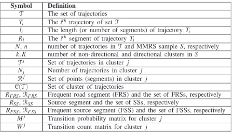
TABLE I: Notations
Symbol Definition
T The set of trajectories
Ti Theithtrajectory of setT
li The length (or number of segments) of trajectoryTi Ri Theithsegment of trajectoryTi
N,n number of trajectories inTand MMRS sampleS, respectively
k,K number of non-directional and directional clusters inS
Tj Set of trajectories in cluster j Nj Number of trajectories in clusterj
Rj Set of points (segments) in clusterj
C(T) Set of cluster of trajectories
RFRS,RF RS Frequent road segment (FRS) and the set of FRSs, respectively RSS,RSS Source segment and the set of SSs, respectively
RFSS,RF SS Frequent source segment (FSS) and the set of FSSs, respectively Mj Transition probability matrix for clusterj
Wj Transition count matrix for clusterj
{T1,T2, ...,TN} is given. Then, for a given partial trajectory
Tp=hL
1,L2, ...,Lmi, the goal is to predict the future road
segments Li, where i,m∈Zand i≥m+1.
B. Distance Measure (trajDTW)
Most of the existing distance measures for trajectory similar-ity are not suitable for a large number of overlapping trajecto-ries in a dense road network due to the use of either the number of overlapping road segments or maximum/minimum distance between trajectories in their computation. In our work, we
use the Dijkstra baseddynamic time warping(DTW) distance
measure, trajDTW [34] to compute trajectory similarities which is suitable for a large number of overlapping trajectories in a dense road network. The superiority of the trajDTW
over the traditionally used dissimilarity with length (DSL)
and Hausdorff distance measures is demonstrated in [34]. The trajDTW is a normal DTW algorithm with a Dijkstra distance
matrix based cost function and a window parameterw, which
is set to the half of the length of shorter of two trajectories, to avoid overestimation of the actual distance. As the road
network is static, the distance matrixDall (of size (|E|×|E|)
of all the edgesE inGRN can be pre-computed and stored.
C. Non-directional trajDTW
The directionality of trajectories can result in misleading distances among them, which in turn may cause incorrect clustering results. For example, suppose there are two
trajec-toriesT1 andT2, which follow the same route but in opposite
directions, then the distance between them considering their directions in computation will be higher than the distance computed without considering their directions. Therefore, if their movement direction is considered as part of the distance
computation, T1 and T2 may not be grouped in the same
cluster. The problem of incorrect distance measure due to the movement direction of trajectories is addressed by reversing one of them (reversing the sequence order so that the starting point becomes the ending point and vice versa), and taking the minimum distance between the first and second trajectory, and the first trajectory and second reverse trajectory. This distance is called non-directional trajDTW [34], and is given as:
(2)
non-directional trajDTW(T1,T2)
D. The clusiVAT Algorithm
In our proposed framework, we modify the clusiVAT al-gorithm and use it for efficiently clustering large volumes of
trajectory data. The clusiVAT model finds its root in thevisual
assessment of cluster tendency (VAT) [35] andimproved VAT
(iVAT) [36] algorithms. The VAT and iVAT algorithms reorder
the input dissimilarity matrixDN (forN datapoints) toD∗N (in
VAT) andD′∗N (in iVAT), respectively, using a modified Prim’s
algorithm (for finding a minimum spanning tree (MST)) and
by applying a graph theoretic distance conversion, such that the dark blocks along the diagonal of the reordered image
I(D∗N)(orI(D′∗N)) potentially represent different clusters. VAT
and iVAT seem to work well for relatively small size datasets.
However, both have space and time complexity of O(N2),
which limits their usefulness for input matrix sizes of an order
of 105 and so. To overcome this limitation, an intelligent
sampling based scalable clustering algorithm, clusiVAT [5] was proposed for visual cluster tendency assessment and subsequent clustering on big data. The essential steps in clusiVAT are:
Maximin Random Sampling (MMRS):MMRS sampling
begins by findingk′ (an overestimate of k) Maximin samples
(distinguished objects), which are furthest from each other
in the input data. Then, each object in the input data is grouped with its nearest Maximin sample with NPR. This
step divides the entire data into k′ groups. Then, a sample
S of size n (just a small fraction of input data size, N) is
built by selecting a proportional number of random data points
(Random sampling (RS)) from each of the k′ groups. Hence
the term MMRS is used for the overall process. Any value ofk′
which overestimates assumed true number of clusters (k) i.e.,
k′≥kshould be a good choice [37]. Forn,n=a few hundred
datapoints is a reasonable choice for most datasets [38].
Step 2. iVAT: The iVAT is applied to the small Dn
(computed from n<<N samples) distance matrix to obtain
its reordered distance matrix D′∗n. The image I(D′∗n) usually
provides an useful estimate ofk, without the need to compute
the very large distance matrix DN.
Step 3. Clustering: Single linkage clusters are always aligned partitions in the VAT/iVAT reordered matrices. Having
the estimate of k from the previous step, we cut the k−1
longest edges in the iVAT-built MST of Dn, resulting in k
single linkage clusters. If the dataset is complex and clusters
are intermixed, cutting thek−1 longest edges may not always
be a good strategy as the outliers, which are typically furthest
from normal clusters, might comprise most of thek−1 longest
edges of the MST, resulting in misleading partitions. A useful approach in such a scenario is to manually select the dark blocks, and find the sample trajectories representing each dark block. Another useful approach [39] to obtain clusters is by cutting the MST using cut threshold magnitudes ordered by
edge distances d in the MST. The cluster boundaries are
defined by those indicesz, which satisfy
dz>α×mean(d), (3)
where α is a parameter that controls how far two groups
of data points should be from each other to be considered
as separate clusters. Smaller values of α represent tighter
cluster boundaries, while large values ofαcreate loose cluster
boundaries. The procedure to find an optimal value of α is
described in [39].
Step 4. Nearest Prototyping Rule (NPR):Thek-partitions
of thensamples are non-iteratively extended to the remaining
(non-sampled)N−n objects in the dataset using the nearest
prototyping rule.
The implementation and pseudocodes of the trajDTW, VAT, iVAT, and clusiVAT algorithms are well documented in the literature, and are not produced here for brevity.
E. Markov Chain Model
AMarkov chain(MC) is the simplest form of the Markov
process in which only the current state determines the proba-bility of transitioning to the next state. Specifically, a Markov
chain model is defined by the transition matrix M, which
contains the transition probabilities associated with various state changes. In a road network, an MC is constructed by assigning a state to each node or road segments in the given
road network. For any two adjacent road segmentsRi andRj
in road network GRN, the transition probability of traveling
fromRi toRj in one step is given by
pi j=
#(Ri,Rj)
#(Ri) , (4)
where #(Ri,Rj)is the number of trajectories that contain the
sequence{Ri,Rj}and #(Ri)is the total number of trajectories
that passes throughRi. For each pair of adjacent road segments
in the graph network, the transition probabilities can be
computed using (4), and stored as entries Mi j of transition
probability matrix M (of size |E|×|E|). We also define a
transition count matrix W whose i j-th entry Wi j represents
the number of trajectories that contain sequence{Ri,Rj} i.e.,
Wi j=#(Ri,Rj). We utilizeW in computing a representative
trajectory for each cluster in our work.
IV. PROPOSEDFRAMEWORK
This section presents our proposed framework for trajectory prediction. The frequent route patterns of moving objects can be discovered by clustering their historical trajectories. In our framework, we employ a modified version of the clusiVAT algorithm that we called Traj-clusiVAT. In Traj-clusiVAT,
we introduce a representative trajectory for each cluster to
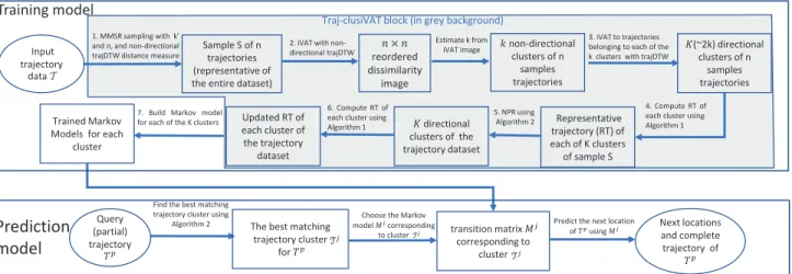
improve the performance of NPR for trajectory clustering. We also modify the NPR technique in Traj-clusiVAT to improve its performance for trajectory prediction. The Traj-clusiVAT algorithm partitions the trajectories into different groups of similar trajectories, based on the trajDTW distance measure. After clustering trajectories, we train a first-order Markov chain model for each cluster using only the trajectories con-tained therein. Then, these trained Markov chain models are used for trajectory prediction. The architecture of our proposed framework consisting of both training and prediction models is illustrated in Fig. 1.
A. Training Model
The essential steps of our training model are: (i) MMRS sampling on input trajectory data, (ii) VAT/iVAT and clustering
Sample S of n trajectories (representative of the entire dataset)
× reordered dissimilarity image !non-directional clusters of n samples trajectories "(~2k) directional clusters of n samples trajectories "directional clusters of the trajectory dataset 1. MMSR sampling with k’
and n, and non-directional trajDTW distance measure
2. iVAT with non-directional trajDTW
Estimate k from iVAT image
3. iVAT to trajectories belonging to each of the k clusters with trajDTW
Representative trajectory (RT) of each of K clusters of sample S Updated RT of each cluster of the trajectory dataset 4. Compute RT of each cluster using Algorithm 1 5. NPR using
Algorithm 2
Trained Markov Models for each
cluster
6. Compute RT of each cluster using Algorithm 1 7. Build Markov model
for each of the K clusters
The best matching trajectory cluster
for #$
transition matrix %&
corresponding to cluster
Find the best matching trajectory cluster using
Algorithm 2
Choose the Markov
model %&corresponding
to cluster
Predict the next location
of #$using %& Input trajectory data T Next locations and complete trajectory of #$ Training model
Prediction
model
Traj-clusiVAT block (in grey background)
Query (partial) trajectory
#$
Fig. 1: The architecture of our proposed framework. the trajectory sample using non-directional trajDTW to obtain
k non-directional clusters (iii) VAT/iVAT and clustering the
trajectories of each of thekclusters using trajDTW resulting in
K(approx. 2k) directional clusters (iv) Computerepresentative
trajectory (RT) of each cluster, (v) Assign remaining
non-sampled trajectories toKclusters using NPR (vi) Re-compute
the RT of each cluster, and (vii) Train a first-order Markov chain model for each cluster. The first six steps constitute the Traj-clusiVAT clustering algorithm. Below, we explain each step corresponding to the steps as shown in Fig. 1.
1) MMRS sampling on input trajectory data
The first step consists of extracting a small, representative sample from the large trajectory data using MMRS sampling with non-directional trajDTW distance measure on input
tra-jectory data T. The aim of this step is to find the most
distinguished vehicle routes in a given road network. The use of non-directional trajDTW circumvents the selection of more than one trajectory from the same route. In this way, the Maximin (first) step of MMRS ensures that MMRS samples
contain the k′ MM trajectories of the most distinguished
vehicle routes. This divides the trajectory data T into k′
partitions. Then, additional trajectories are randomly chosen
from each of the k′ partitions to generate a sample S of n
trajectories. The MMRS intelligently chooses n trajectories
which are almost equally distributed among the different
clusters as the N trajectories in the big trajectory data, i.e.,
it obtains a representative sample.
2) Clustering trajectory samples using non-directional tra-jDTW
The previous step provides a trajectory sampleScontaining
n trajectories. In this step, the iVAT is applied to the distance
matrix Dn returning a reordered distance matrixD′∗n, and the
cut magnitudes of the MST links, d. The visualization of
D′∗n using I(D′∗n) suggests the number of clusters k present
in the dataset. Thekpartitions can be obtained by cutting the
k−1 edges or by cutting the MST cut magnitudes d using
cut threshold α, as mentioned in Section III-D. The
non-directional trajDTW distance measure is used in this step to
cluster the ntrajectories in order to avoid incorrect clustering
due to the movement direction of trajectories, as mentioned in
Section III-C). From here on, we denote k as the number of
non-directional clusters.
3) Clustering trajectories in each cluster using trajDTW
The previous step clusters the trajectories based on their path similarity computed using non-directional trajDTW, which ensures that the trajectories that are in opposite direc-tions, but follow similar routes, are clustered together. Since Markov chain models are used in our framework to model the trajectories of each cluster, their transition probabilities may be misleading for trajectory prediction task for clusters in which the number of trajectories in opposite directions is approximately equal. To circumvent this problem, we use the trajDTW (directional) distance measure for the sample trajectories of each cluster obtained in the previous step to separate the trajectories going in opposite directions using a second application of the iVAT algorithm, which in turn, gives
K∼2kdirectional clusters.
4) Computing the RT of each cluster
In the NPR (next) step of clusiVAT, the non-sampled trajec-tories are assigned to one of the clusters (found in the previous step) based on their (nearest) distances from each cluster. For
a fast and reliable implementation of NPR, we require a
repre-sentative trajectory(RT) for each cluster that best describes the
cluster, much like centroid-based clustering methods identify a representative "center" for each cluster. However, it is not possible to compute the centroid of trajectory clusters in a conventional way due to different lengths of trajectories in each cluster. Existing methods of calculating RT [40]–[43] in the literature either compute the mean trajectory using the average of GPS coordinates [41], [43]; or select a trajectory from each cluster which minimizes the dissimilarity between all the trajectories within the cluster [40], [42]; or pick a random trajectory [42] from each cluster, and designates it as the RT. These methods incur a large computational cost to compute an RT that minimizes the dissimilarity among all the trajectories. Additionally, RTs computed using these methods do not show all the possible variability inside a cluster [44]. The mean trajectory computed from trajectories of different lengths may be inaccurate; thus, it may not be a good representative of the cluster.
Our scheme generates animaginary trajectory(IT) (it may
4 1 2 3 5 6 7 8 9 4 1 5 6 7 9 4 1 5 6 7 9 4 1 2 3 5 6 7 8 9 4 1 5 6 7 9 (a) (b) (c) (d) (e)
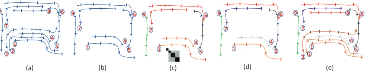
Fig. 2: A simple illustration of Traj-clusiVAT for trajectory clustering for each cluster that describes the major movement patterns
of the trajectories belonging to that cluster. The pseudocode of our proposed method to compute RT for each cluster is shown in Algorithm 1. Below, we explain our RT computing algorithm.
First, we compute the transition count matrixWi for each
cluster Ti using the trajectories in that cluster (line 2). Then,
for each cluster Ti, we compute the set of frequent road
segments (FRSs) Ri
FRS using the MinT threshold (line 3).
The road segments in cluster Ti which contains at least
MinT% of the total trajectories in that cluster are assigned
toRi
FRS. Then, a set offrequent source segments(FSSs)RiFSS
is identified (line 4). A source segment RiSS is a FSS,RiFSS,
if at least MinT% of total trajectories in the cluster originate
from RiSS i.e, RiFSS∈Ri
SS, RiFSS∈RiFRS. Then for each FSS
Ri
FSS∈RiFSS (line 5), an imaginary trajectory ITi(RiFSS) is
initialized with Ri
FSS assigning it as current segment Rcurrent
(lines 6−7). In lines 9−17, we compute the next RSRnext
based on the highest transition count from current RSRcurrent
using transition count matrix Wi (refer to Section III-E) . If
Rnext∈RiFRS, then Rnext is added to current ITi(RiFSS), and
assigned as Rcurrent to compute new Rnext. The steps in lines
9−18 are repeated until Rnext is non-FRS, which means an
imaginary trajectory is an ordered sequence of only frequent
road segments in that cluster. A total of |Ri
FSS| imaginary
trajectories will be generated for each clusterTi, corresponding
to eachRiFSS∈Ri
FSS. We define a variableCount_score(line 8)
for each imaginary trajectoryITi(RiFSS), RiFSS∈Ri
FSS, which
is the sum of the total transition counts of each RS∈ITi(RiFSS)
in cluster Ti. Among all |Ri
FSS| ITs, the one which has the
highest Count_score will be assigned as RT(Ti) of cluster
Ti (line 20). As the RT(Ti) is the sequence of FRS with
highest Count_score, it contains major movement behaviour
or patterns of the trajectories belonging to the cluster Ti.
Algorithm 1 does not require the computation of dissim-ilarity among all trajectories in that cluster to compute RT, which is computationally expensive for large size clusters. In contrast, Algorithm 1 is a novel algorithm to compute RT based on the transition count matrix of each cluster.
5) Assigning non-sampled trajectories to identified K clus-ters using NPR
The previous step gives representative trajectoryRT(Ti)for
each clusterTi. In this step,N−nnon-sampled trajectories are
assigned to one of theKdirectional clusters based on the NPR.
The NPR method in clusiVAT uses the trajDTW (directional) distance measure to assign non-sampled trajectories to one of
theK clusters based on their nearest distance from (clustered)
Algorithm 1 Computing the RT of each cluster
Input: Tj- set of trajectories in cluster j, N
j- number of
tra-jectories in cluster j, Rj- set of road segments in cluster j, C(T) ={T1, ...,TK}- set of cluster of trajectories, MinT- FRS
threshold
1: foreach clusterTi∈C(T)do
2: Compute transition count matrixWifor clusterTi
3: Compute FRSs, Ri F RS, from Ri, RiFRS = {Rj∈Ri}#(Rj)≥MinT×Ni 4: Compute FSSs,Ri FSSfromRiSS ={Rj}Rj∈RiSS∈RiFRS 5: foreach FSSRi FSS∈RiFSS do
6: AssignRiFSSas current road segment,Rcurrent=RiFSS
7: Initialize an imaginary trajectory IT with Rcurrent,
ITi(RiFSS) ={Rcurrent}
8: Count_score(ITi(RiFSS)) =0
9: whileeach RS ofITi(RiFSS)∈Ri FRS do
10: Compute next RS,Rnext=argmax Rj∈Ri
{Wcurrenti ,j}
11: ifRnext∈RiFRS then
12: AppendRnext to existingITi(RiFSS)
13: Rcurrent=Rnext
14: Count_score(ITi(RiFSS))+=Wcurrenti ,next
15: else
16: break;
17: end if 18: end while 19: end for
20: SelectITi(RiFSS) with the highestCount_score(ITi(RiFSS))
from all|Ri
FSS|ITs ofTi, and assign it as RT for clusterTi
21: end for
Output:RT(Ti)- RT for each clusterTi∈C(T)
Algorithm 2 Hybrid NPR Method
Input:Tq- query trajectory,Mj- transition probability matrix for
cluster j,RT(Tj)- representative trajectory for cluster j
1: Compute the path probabilityPi(Tq)of query trajectory in each
clusterTi usingMi and Eq. 5.
2: ifany(Pi(Tq)>0then ⊲ifTq is present in any clusterTi
3: Select the cluster c with the highest Pi(Tq) i.e., c=
argmax
Ti∈C(T)
{Pi(Tq)}
4: else
5: Compute the trajDTW distance of Tq from RT(Ti), yi=
tra jDTW(Tq,RT(Ti)), for each clusterTi∈C(T)
6: Select the cluster c with the minimum yi i.e., c =
argmin
Ti∈C(T)
{yi}
7: end if
8: Assign theTq with clusterc(orTc).
sample trajectories. However, trajDTW distance of a non-sampled trajectory to cluster RTs may not be an appropriate
measure for the NPR step due to its dependency on thelength
of trajectories, as explained by the following example.
Suppose Ta is a non-sampled trajectory in T, and RT(Ti)
andRT(Tj)are the RT of clusterTi andTj, respectively. Let
Ta be a sub-trajectory of RT(Ti) i.e., Ta is fully contained
in RT(Ti). Since the trajDTW distance relies on a warping
window size parameterw, thetra jDTW(Ta,RT(Ti))not only
depends on the coordinates of RSs of both trajectories, but
it also depends on the length of Ta and RT(Ti). Moreover,
tra jDTW(Ta,RT(Ti)) also varies depending on the position
of Ta in RT(Ti) due to window parameter. Therefore, even
if Ta⊑RT(Ti) and Ta6 RT(Tj), Ta may be incorrectly
as-signed to cluster Tj instead of Ti iftra jDTW(Ta,RT(Ti))≥
tra jDTW(Ta,RT(Tj)). Here is such an example from
T-Drive data. Suppose T1=h70,75,90,89,88iis a non-sample
trajectory, and RT(T1) =h16,18,68,70,75,90,89,88i and
RT(T2) =h68,70,75,91,92iare RTs of two clusters, where
each trajectory is represented by a sequence of road segments’ IDs of Beijing road network (Refer to Section VI-A). The
trajDTW distances are: tra jDTW(T1,RT(T1)) =0.3482 and
tra jDTW(T1,RT(T2)) =0.2767. Therefore, although T1 is
a sub-trajectory of RT(T1), it will be assigned to cluster
T2 based on nearest trajDTW distance. Such assignments of
non-sampled trajectories to (incorrect) cluster may include outlier trajectories or road segments in that cluster, which may adversely affect Markov chain modeling, and consequently, degrade the performance of trajectory prediction.
To address above issue, we propose ahybrid NPR strategy
based on the path probability and trajDTW distance measure.
Hybrid NPR is similar to clusiVAT NPR except for those
non-sampled trajectories, which are sub-trajectory of any of the clusters’ trajectories. The pseudocode of our hybrid NPR method is shown in Algorithm 2. For a query trajectory
Tq={R1,R2, ...,Rl}, we first compute the path probability
Pi(Tq)for each clusterTi, which is defined as
Pi(Tq) = l
∏
j=1 pj(j+1)⇔ l∏
j=1 Mij(j+1). (5)Pi(Tq)>0 means that sequenceTq appears at least once in
clusterTi, whereasPi(Tq) =0 means that sequenceTqis not
present in cluster Ti. If the sequence Tq is present in any
cluster Ti i.e., any(Pi(Tq))>0, then Tq is assigned to the
cluster with the highest path probability. If the sequence Tq
is not present in all clusters Ti i.e., all(Pi(Tq)) =0, then Tq
is assigned to the cluster based on its (minimum) trajDTW
distance from RTs. All non-sampled trajectories in T are
assigned to one of the K clusters using Algorithm 2.
6) Recompute the RT of each cluster after NPR
The assignment of all non-sampled trajectories to one of the
K clusters in the NPR step updates each cluster with new
tra-jectories. Therefore, a representative trajectory is recomputed for each updated cluster using Algorithm 1.
7) Train Markov chain model
For each of the K clusters, we build a first-order Markov
chain model using the trajectories of that cluster. Specifically,
we compute the transition probability matrix Mi for each
clusterTc.
For a basic understanding of Traj-clusiVAT algorithm, we
graphically explain its steps on a small trajectory data T, as
shown in Fig 2. An input trajectory dataT containing N=9
trajectories is shown in Fig 2 (a). The MMRS sampling onT
with non-directional trajDTW in the first step returns a MMRS
sampleS containingn=6 sample trajectories{1,4,5,6,7,9},
which are well-distributed in sampleS, as shown in Fig 2 (b).
In the next step, iVAT is applied toSusing the non-directional
trajDTW distance measure, which clusters the trajectories based on the path similarity irrespective of their movement directions. The iVAT image in Fig 2 (c) shows four dark blocks
along its diagonal, which indicates four clusters in sampleS.
Having an estimate ofk=4, sampleSis partitioned into four
(non-directional) clusters {{1,4},{5},{6,7},{9}}, as shown
with four different colors in Fig 2 (c). Then, the trajectories in each cluster going in opposite directions are separated using the iVAT with the trajDTW distance measure, which gives
K=6 directional clusters{{1},{4},{5},{6},{7},{9}}, each
cluster is shown with a different colour in Fig 2 (d). Since there is only one trajectory in each cluster in this case, they are the RTs for corresponding clusters. In the next step, non-sampled
trajectories{2,3,8}are assigned to one of the 6 clusters using
NPR (Algorithm 2), which partitions the complete data into 6 clusters{{1,2,3},{4},{5},{6,8},{7},{9}}. Trajectory 4 is in
different cluster than{1,2,3}due to opposite direction. Then,
a Markov chain model is trained for each cluster using the trajectories of that cluster.
B. Prediction Model
For a given partial trajectory Tp=hL1,L2, ...,Lmi, we first
estimate the best matching representative clusterTcusing our
hybrid NPR approach, and then choose the corresponding
Markov model of the cluster to predict the next locations Li,
i≥m+1. Using the cluster Tc, the location L
m+1 that the
object will arrive at next is given by
Lm+1=arg max
Lj∈Rc
{pm j} ⇔arg max
Lj∈Rc
{Mm jc } (6)
The Tp is updated with the next predicted location L
m+1.
Then, the updated Tp is used to estimate the best matching
cluster and the corresponding MM is used to predict the next location. The complete trajectory is predicted by computing next locations in a sequential manner using these steps.
V. TIMECOMPLEXITY
In this section, we discuss the time complexity of our proposed Traj-clusiVAT based TP approach. The first step in
Traj-clusiVAT is the selection of k′ distinguished trajectories
which are at maximum distance from each other. This step
has the time complexity ofO(k′N), wherek′ is a user-defined
parameter for an overestimate of the number of clusters in the input trajectory data and is usually chosen to be (inessentially) large (usually 50 to 200). The next step is to randomly select
n trajectories from k′ NPR groups to get a sample S. The
computation of distance matrix Dn and VAT on a sample S
computation of Dn and VAT on S is pretty fast and takes
just a small fraction of the total run time of Traj-clusiVAT. The trajDTW distance measure uses Dijkstra’s shortest path distance in the standard DTW algorithm. Its best, average
case complexity with binary heaps is O(|E|+|V|log|V|)[45].
For two trajectories of length l1 and l2, standard DTW has
time complexity of O(l1l2). Remark- There are approximate
algorithms such as FastDTW [46] which have a linear time complexity in the average length of trajectories, however, we have not used this implementation in our experiments. The
NPR step in Traj-clusiVAT has complexity of O(n(N−n)).
The computation of RTs has linear time complexity inK. The
construction of a Markov model for each cluster is a simple
and fast process, which hasO(K)time complexity andO(|E|2)
space complexity.
VI. EXPERIMENTS
In this section, we conduct an extensive experimental study on two real-life, vehicle trajectory datasets to evaluate the performance of our proposed framework. We first describe the datasets, their preprocessing, evaluation metrics and com-putational protocols adopted in our empirical study, and then present the experimental results.
A. Datasets
We performed our experiments on two real trajectory datasets.
1) T-Drive taxi trajectory data [47]
This trajectory dataset is obtained from the T-Drive project
which contains one-week trajectories of 10,357 taxis during
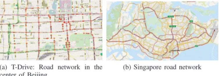
the period of Feb. 2 to Feb 8, 2008 within Beijing, China. The total number of points is about 15 million and the total distance of the trajectories is 9 million kilometres. In our experiment, we have taken a subset of this dataset, which contains trajectories from a road network in the center of Beijing city, as shown in Fig. 3(a). This road network consists of 100 nodes and 141 road segments (edges). The average sampling interval is 177 seconds with an average distance of about 623 meters, which is quite large for a city traffic environment as the length of many road segments is smaller than the average sampling distance.
2) Singapore taxi trajectory data
This dataset consists of the trajectories of more than 15,000
taxis collected over a duration of 1 month from a road network in Singapore City, as shown in Fig. 3(b). This dataset is very dense as it consists of more than 370 million GPS logs. The general format of each data point is as follows: {Time Stamp, Taxi Registration, Latitude, Longitude, Speed, Status}. The Status field contains information about the occupation state of
Taxi, such asFREEandPOB(Passenger on Board). In order
to extract each individual taxi’s trip from the raw data, we
detect the following sequence: starting from FREE to POB
and ending from POB to FREE, using the trip extraction
framework presented in [48]. This road network consists of 1641 nodes and 2941 edges, with an average edge length of 350m.
(a) T-Drive: Road network in the center of Beijing
(b) Singapore road network
Fig. 3: Road networks used in our trajectory prediction exper-iments
TABLE II: Training and test set description
T-Drive Taxi Singapore Taxi Training Set 35,501 1,955,573
Test Set 7,904 1,303,717
Total trajectories 43,405 3,259,290 Data Pre-processing
To obtain the trajectories as a sequence of road segments, we use the popular open source map matching tool GraphHop-per [49], which provides an implementation of the approach presented in [50].
After pre-processing, we have N=43,405 trajectories in
the T-Drive data whose lengths lie in the range of 5 to 200 road segments and have an average of 14 road segments, and
N=3,259,290 (3.26 million) trajectories in the Singapore
data whose lengths lie in the range of 10 to 250 road segments and have an average of 22 road segments. To prepare training and test sets for both datasets, we first divided the trajectories into two sets based on the day of week viz., weekdays and weekends, during which the trip is being made. For the one-week T-Drive data, we considered trajectories during first 4 weekdays (Monday to Thursday) and first weekend day (Saturday) as the training set, and trajectories during the remaining days (Friday and Sunday) of that week as the test set. For the one-month Singapore data, we considered 60% trajectories randomly as training set and remaining 40% as the test set, for both weekdays and weekend data. The size of training and test sets for both trajectory datasets is shown in Table II. We split each trajectory in a test set into two halves. The first half is used as a partial trajectory (or query trajectory) for predicting its future locations and the second half is used as ground truth to validate our predictions. The distribution of predicted trajectories (second half) in the T-Drive and Singapore test sets is shown in Fig. 4.
B. Evaluation Metrics
In our experiments, we assess the performance of our framework for next location prediction (also known as
one-1 4 7 10 13 16 19 22 25 28
Length of predicted trajectory 0 200 400 600 800 1000 1200 1400 1600
Nos. of predicted trajectories
(a) T-Drive Taxi
0 5 10 15 20 25 30 35 40 45 50
Length of predicted trajectory 0 1 2 3 4 5 6
Nos. of predicted trajectories
105
(b) Singapore Taxi
Fig. 4: Trajectory distribution of predicted trajectories based on their lengths.
step prediction) and long-route prediction using following evaluation metrics:
1) Prediction Accuracy (PA)
The PA is the ratio of correctly predicted locations to the total possible number of predicted locations for each trajectory.
Given a predicted trajectory sequence Tpred={L1,L2, ...,Lm}
and a true (actual) trajectory sequenceTtrue={R1,R2, ...,Rm},
the prediction accuracy is defined as
PA= 1 |Tpred| m
∑
j=1 H(Lj,Rj), (7)whereH(Lj,Rj)is 1 ifLj=Rj, else 0. The average prediction
accuracy is the average of PA for all predicted trajectories in test set Ttest.
2) Prediction Rate (PR)
The PR is the number of trajectories that are correctly predicted over the total number of trajectories in test set. It is defined as PR= 1 |Ttest| |Ttr|
∑
j=1 H(Tpredj,Ttruej), (8)whereH(Tpredj,Ttruej)is 1 ifTpredj =Ttruej, else it is 0. 3) Distance error (DE)
Another important performance metric of the long-term pre-diction system is the capability of continuous route prepre-diction. Thedistance erroris defined as the average spatial (Haversine) distance between predicted and actual routes. Given a route
sequence Tpred andTtrue, the distance error between them is
given as DE(Tpred,Ttrue) = 1 |Tpred| m
∑
j=1 DH(Lj,Rj), (9)whereDH(Lj,Rj)is the Haversine [51] distance between two
locations (road segments).
4) One-step accuracy (OA)
This is the ratio of correctly predicted next locations to the total predicted next locations for all trajectories in test set.
5) One-step distance error (ODE)
The ODE defined as the average distance error for one-step (or next location) prediction.
C. Comparison Methods
Among the plethora of MM and clustering based TP meth-ods available in the literature, we implemented these two approaches for comparison.
1) Mixed Markov model (MMM) based TP [8]: MMM was proposed as an intermediate model between standard MM and HMM which can encompass all types of movement behaviour present in an input trajectory data. It first clusters the trajectories into groups using the EM algorithm, and then builds an MM for each group, which is subsequently used for prediction. This approach was tested on synthetic and real datasets in [8], which
showed 74.1% accuracy for MMM, in comparison to
16.9−45.6% for MM and 2.4−4.2% for HMM.
2) NETSCAN-based TP: The well-known density-based algorithm DBSCAN and its variants [32], [52]–[54] have
been used extensively as a trajectory clustering method for location prediction [11]. However, they are not suitable for a large number of trajectories as computation
of the distance matrix is time intensive. Kharratet al.[9]
proposed a trajectory clustering relative of DBSCAN, called NETSCAN which first finds dense road segments based on the moving object counts, merges them to form dense paths on the road network, and then assigns sub-trajectories to the dense paths based on a measure of similarity. This method requires two user-defined param-eters: a density threshold – the minimal required density for transition, and a similarity threshold- the maximum density difference between neighbouring road segments. We implement NETSCAN to cluster trajectories into dense road segments, then built an MM for each cluster, and subsequently used them for TP.
Our proposed method and the baseline methods discussed above are also comparable in terms of prediction time (which will be discussed shortly). They all require a short prediction time and satisfy the requirement of real-time prediction.
D. Computation Protocols
All algorithms were coded in MATLAB on a PC with the following configuration; OS: Windows 7 (64 bit); processor:
Intel Core i7−4770 @3.40GHz; RAM: 16GB. We denote
the comparison approaches of [8] as MMM, of [9] as
NETSCAN, and our clusiVAT based TP approach as Traj-clusiVAT. All three algorithms were applied to T-Drive data. The MMM method requires the computation and storage of
an intermediate matrix of size |E|×|E|×N, which is very
large for Singapore data (due to large |E| and N), so we
can not apply MMM to the Singapore data. However, we have compared it with NETSCAN-TP and Traj-clusiVAT-TP on a subset obtained from a smaller part of the Singapore road network. The number of mixed models of MMM was determined using 10-fold cross-validation. The NETSCAN parameter, density threshold and similarity threshold, were chosen to get as many dense paths (with at least six road segments) as the number of clusters we get using the Traj-clusiVAT algorithm, for a fair comparison. The parameters for
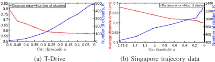
Traj-clusiVAT were chosen as follows:k′=150,n=500, and
α =0.05 for the T-drive data, and k′=300, n=1000, and
α=0.06 for the Singapore data, andMinT =30% for both
data. It is worth noting that, unlike other clustering algorithms, the clusiVAT algorithm is relatively insensitive to the choice
ofk andn [5]. Moreover, we study the effect of α on
Traj-clusiVAT performance in our experiments.
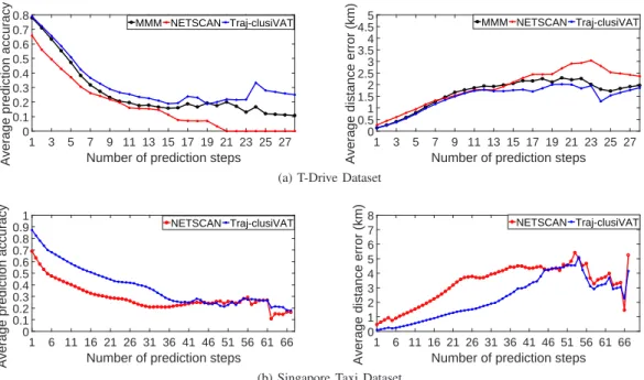
E. Comparison of MMM, NETSCAN, and Traj-clusiVAT for Long-term predictions
Long-term prediction, also known as continuous route pre-diction, is a challenging and ongoing research problem in TP. In this experiment, we compare the performance of the MMM, NETSCAN, and Traj-clusiVAT-based prediction approaches
form-step predictions. Specifically, this refers to predicting the
nextmlocations for a given partial trajectory. Fig. 5 shows the
1 3 5 7 9 11 13 15 17 19 21 23 25 27 Number of prediction steps 0 0.1 0.2 0.3 0.4 0.5 0.6 0.7 0.8
Average prediction accuracy
MMM NETSCAN Traj-clusiVAT
1 3 5 7 9 11 13 15 17 19 21 23 25 27
Number of prediction steps 0 0.5 1 1.5 2 2.5 3 3.54 4.55
Average distance error (km)
MMM NETSCAN Traj-clusiVAT
(a) T-Drive Dataset
1 6 11 16 21 26 31 36 41 46 51 56 61 66 Number of prediction steps 0 0.1 0.2 0.3 0.4 0.5 0.6 0.7 0.8 0.91
Average prediction accuracy
NETSCAN Traj-clusiVAT
1 6 11 16 21 26 31 36 41 46 51 56 61 66 Number of prediction steps 0 1 2 3 4 5 6 7 8
Average distance error (km)
NETSCAN Traj-clusiVAT
(b) Singapore Taxi Dataset
Fig. 5: Average prediction accuracy and average distance error comparison by prediction steps error (right panels) of all three algorithms for increasing
pre-diction steps. The graphs in Fig. 5 support these observations: (i) First, the Traj-clusiVAT outperforms the MMM and NETSCAN-based TP approaches based on the average PA and DE for the T-Drive data, as shown in Fig. 5(a). The higher the number of prediction steps, the larger the gap between clusiVAT and other two approaches. This means that the Traj-clusiVAT performs better not only for short-term predictions but it performs even better than the other two approaches for long-term predictions. This is probably because Maximin sampling in Traj-clusiVAT finds the trajectories which are furthest from each other. As the trajDTW distance measure yields higher distances for longer trajectories, Maximin sam-pling tends to pick longer trajectories in its output sample which form separate clusters in subsequent steps. The Markov models trained on these clusters after the NPR step contain all movement behaviours similar to those longer trajectory patterns. Therefore, if a query trajectory pattern is not available in any cluster, which is frequent for longer query patterns, then it is assigned to a cluster based on its nearest distance from all cluster RTs. This will assign longer query trajectories to any of the clusters containing longer trajectory patterns, and subsequently, corresponding MMs trained on these clus-ters contribute towards better predictions for longer query trajectories during the prediction phase. On the other hand, the longer movement rules cannot be easily represented by Markov-based models, especially for irregular trajectory data, due to uncertainty in movement behaviours of vehicles in a complex road network. As there are only a few prediction trajectories available for the T-Drive test set whose lengths are greater than 16 as shown in Fig. 4 (a), the performance of all approaches cannot be considered conclusive for longer
prediction steps (m>16)based on their performance on the
T-drive data.
(ii) Fig. 5 (b) shows that the Traj-clusiVAT model also
performs better than the NETSCAN-based method based on the average PA and DE values for the Singapore data. The gap between the NETSCAN and Traj-clusiVAT plots increases until 31th prediction step and then reduces with longer pre-diction steps. This may be because the trajectory clusters obtained by NETSCAN are usually spread over the entire road network [34], which results in longer dense paths. Therefore, its performance becomes competitive with Traj-clusiVAT for longer prediction lengths compared to its short-term prediction performance.
(iii) It can be observed that difference in performance of the NETSCAN method and the proposed method is less for short-term and more for long-term prediction for T-drive data, whereas it is opposite for the Singapore data. This is because the T-drive subset contains many parallel and perpendicular road segments and intersections that span only a small road network (Beijing city center), whereas, Singapore data con-tains relatively longer and straight (fewer intersections) trajec-tories (compared to T-Drive subset) that span entire Singapore city road network (significantly bigger than Beijing city center road network). Therefore, incorrect predictions cause relatively smaller distance error for T-Drive data as compared to distance error for Singapore taxi dataset. NETSCAN’s clusters for Singapore dataset are ordered sequences of only a few but longer and straight dense paths, therefore, it modeled long trajectories better for Singapore dataset, and in turn, performed better for long-term prediction as compared to the T-Drive dataset.
(iv) The performance of all three approaches deteriorates as the prediction step increases. This may be because the number of frequent trajectory patterns obtained is small for long-term predictions, which do not contain enough information
to forecast future locations1.
1And the other reason, as Niels Bohr said, is that "it is very hard to predict,