energies
ArticlePrediction of Hydropower Generation Using Grey
Wolf Optimization Adaptive Neuro-Fuzzy
Inference System
Majid Dehghani1, Hossein Riahi-Madvar2, Farhad Hooshyaripor3, Amir Mosavi4,5 , Shahaboddin Shamshirband6,7,* , Edmundas Kazimieras Zavadskas8 and
Kwok-wing Chau9
1 Technical and Engineering Department, Faculty of Civil Engineering, Vali-e-Asr University of Rafsanjan, P.O. Box 518, Rafsanjan 7718897111, Iran; [email protected]
2 College of Agriculture, Vali-e-Asr University of Rafsanjan, P.O. Box 518, Rafsanjan 7718897111, Iran; [email protected]
3 Technical and Engineering Department, Science and Research, Branch, Islamic Azad University, Tehran 1477893855, Iran; [email protected]
4 Institute of Automation, Kando Kalman Faculty of Electrical Engineering, Obuda University, 1034 Budapest, Hungary; [email protected]
5 School of the Built Environment, Oxford Brookes University, Oxford OX3 0BP, UK
6 Department for Management of Science and Technology Development, Ton Duc Thang University, Ho Chi Minh City, Viet Nam
7 Faculty of Information Technology, Ton Duc Thang University, Ho Chi Minh City, Viet Nam
8 Institute of Sustainable Construction, Vilnius Gediminas Technical University, LT-10223 Vilnius, Lithuania; [email protected]
9 Department of Civil and Environmental Engineering, Hong Kong Polytechnic University, Hong Kong, China; [email protected]
* Correspondence: [email protected]
Received: 31 December 2018; Accepted: 16 January 2019; Published: 17 January 2019 Abstract:Hydropower is among the cleanest sources of energy. However, the rate of hydropower generation is profoundly affected by the inflow to the dam reservoirs. In this study, the Grey wolf optimization (GWO) method coupled with an adaptive neuro-fuzzy inference system (ANFIS) to forecast the hydropower generation. For this purpose, the Dez basin average of rainfall was calculated using Thiessen polygons. Twenty input combinations, including the inflow to the dam, the rainfall and the hydropower in the previous months were used, while the output in all the scenarios was one month of hydropower generation. Then, the coupled model was used to forecast the hydropower generation. Results indicated that the method was promising. GWO-ANFIS was capable of predicting the hydropower generation satisfactorily, while the ANFIS failed in nine input-output combinations. Keywords:hydropower generation; hydropower prediction; dam inflow; machine learning; hybrid models; artificial intelligence; prediction; grey wolf optimization (GWO); deep learning; adaptive neuro-fuzzy inference system (ANFIS); hydrological modelling; hydroinformatics; energy system; drought; forecasting; precipitation
1. Introduction
Hydropower is a renewable source of energy that is derived from the fast reservoir water flows through a turbine. One of the main purposes of dam construction is to generate the hydropower via installation of a hydropower plant near the dam site. The rate of hydropower generation depends on the dam height and the inflow to the dam reservoir. Nonetheless, hydropower is one of the
major sources of power supply in each country. In addition, the power consumption varies strongly during the year. Therefore, an insight on the value of hydropower energy to be produced in the coming months would be an important tool in managing the electricity distribution network and operation of the dam. Consequently, hydropower generation forecasting could be a key component in dam operation. Hamlet et al. [1] evaluated a long-lead forecasting model in the Colombia river and stated that long-lead forecasting model led to an increase in annual revenue of approximately $153 million per year in comparison with no forecasting model. Several researches carried out based on the inflow forecasting to the dam and executing an operating reservoir model to determine the hydropower generation [2–8]. While these researches are promising, some challenges arise during the implementation of these models. First, forecasting the precipitation is needed and in the next step the inflow to the river and then a reservoir model needs to be run. Each step, including the precipitation or inflow forecasting and reservoir modeling, is associated with uncertainty and the results are highly affected by the uncertainty in these models. Second, an optimization algorithm seems to be needed to optimize the parameters of predictive models.
During the past two decades, several artificial intelligent models were utilized for hydrologic model prediction [9] and hydropower stream flow forecasting [10]. Among them, the ensemble models [11–13] and hybrid models [14] have recently become very popular. Recently, to produce novel hybrid models, different optimization algorithms were coupled with these models to improve their performance [15–20]. Among the optimization algorithms, Grey wolf optimization (GWO) has shown promising results in a wide range of application when coupled with machine learning algorithms [21]. Consequently, in this study, to reduce the source of uncertainty, an artificial intelligent model was used for hydropower generation forecasting. For this purpose, the adaptive neuro-fuzzy inference system (ANFIS) was coupled with GWO to forecast the monthly hydropower generation directly based on the precipitation over the basin, the inflow to the dam and the hydropower generation in previous months. This method is capable to facilitate the hydropower generation forecasting. The rest of this chapter is organized as follows. In Section2, the coupled model of ANFIS and GWO and study area are presented. Section3involves the results of hydropower forecasting and its reliability. Finally, Section4includes the conclusion of the study.
2. Methodology and Data 2.1. Study Area
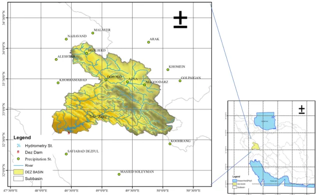
The Dez dam is an arch dam constructed in 1963 on the Dez river southwestern of Iran (Figure1). The dam is 203 m high and has a reservoir capacity of 3340 Mm3. The upstream catchment of the dam with the mean elevation of 1915.3 m above sea level and average slope of 0.0084 has an area of 17,843.3 Km2. The catchment length is about 400 km and ends with the dam reservoir at the outlet. Flow to the reservoir was measured at the Tele-Zang hydrometric station (Figure1). The precipitation stations that were used in the present study include four precipitation stations in the catchment and 10 others around the catchment (Figure1). The hydrometric data was taken from Iran’s Water Resources Management Company (http://www.wrm.ir/index.php?l=EN) and the precipitation data is available from Iran Meteorological Organization (http://www.irimo.ir/eng/index.php). The monthly data used here covered the range of October 1963 to September 2017. The average Inflow to the reservoir and precipitation were calculated and shown in Figure2. According to Figure2, the most precipitation occurred from October to May. Precipitation in the winter accumulated as snowpack over the high mountainous area and in the spring the river flow increased as a result of snowmelt. Summer was dry with almost no considerable precipitation.
Energies2019,12, 289 3 of 20
Energies 2019, 12, 289 3 of 20
Figure 1. Location of the Dez dam and the precipitation stations in Iran.
Figure 2. Average monthly precipitation in the catchment and mean monthly inflow to the Dez dam reservoir.
The primary purpose of the Dez dam is the flood control, hydroelectric power generation and irrigation supply for 125000 ha downstream agricultural area, as well. The Dez hydropower plant consists of eight units with a total installed capacity of 520 MW. The monthly power generation was
# * % ,Tele_Zang AZNA ARAK DOROUD KHOMEIN MALAYER NAHAVAND KOOHRANG ALESHTAR BROUJERD GOLPAIGAN ALIGOODARZ KHORRAMABAD MASJED SOLEYMAN SAFIABAD DEZFUL 50°30'0"E 50°0'0"E 49°30'0"E 49°0'0"E 48°30'0"E 48°0'0"E 47°30'0"E 34 °30 '0 "N 34° 0'0" N 33 °30 '0 "N 33° 0' 0" N 32 °30 '0 "N 32° 0' 0" N Legend % , Hydrometry St. # * Dez Dam Precipitation St. River DEZ BASIN Subbasin
±
#* Persian Gulf Caspian sea 61°30'0"E 58°0'0"E 54°30'0"E 51°0'0"E 47°30'0"E 44°0'0"E 39 °3 0' 0" N 36 °0 '0 "N 32 °3 0' 0" N 29 °0 '0 "N 25 °3 0' 0" N Legend khazar-khalijPoly3 DEZ BASIN Subbasin±
0 200 400 600 800 1000 1200 1400 1600 1800 0 10 20 30 40 50 60 70 80 90 100Jan Feb Mar Apr May Jun Jul Aug Sep Oct Nov Dec
In fl ow ( M m 3) Pr ec ip it at ion ( m m ) Month P (mm) I (MCM)
Figure 1.Location of the Dez dam and the precipitation stations in Iran.
Figure 1. Location of the Dez dam and the precipitation stations in Iran.
Figure 2. Average monthly precipitation in the catchment and mean monthly inflow to the Dez dam
reservoir.
The primary purpose of the Dez dam is the flood control, hydroelectric power generation and irrigation supply for 125000 ha downstream agricultural area, as well. The Dez hydropower plant consists of eight units with a total installed capacity of 520 MW. The monthly power generation was
# * % ,Tele_Zang AZNA ARAK DOROUD KHOMEIN MALAYER NAHAVAND KOOHRANG ALESHTAR BROUJERD GOLPAIGAN ALIGOODARZ KHORRAMABAD MASJED SOLEYMAN SAFIABAD DEZFUL 50°30'0"E 50°0'0"E 49°30'0"E 49°0'0"E 48°30'0"E 48°0'0"E 47°30'0"E 34 °30 '0 "N 34° 0'0" N 33 °30 '0 "N 33° 0' 0" N 32 °30 '0 "N 32° 0' 0" N Legend % , Hydrometry St. # * Dez Dam Precipitation St. River DEZ BASIN Subbasin
±
# * Persian Gulf Caspian sea 61°30'0"E 58°0'0"E 54°30'0"E 51°0'0"E 47°30'0"E 44°0'0"E 39 °3 0' 0" N 36 °0 '0 "N 32 °3 0' 0" N 29 °0 '0 "N 25 °3 0' 0" N Legend khazar-khalijPoly3 DEZ BASIN Subbasin±
0 200 400 600 800 1000 1200 1400 1600 1800 0 10 20 30 40 50 60 70 80 90 100Jan Feb Mar Apr May Jun Jul Aug Sep Oct Nov Dec
In fl ow ( M m 3) Pr ec ip it at ion ( m m ) Month P (mm) I (MCM)
Figure 2. Average monthly precipitation in the catchment and mean monthly inflow to the Dez dam reservoir.
The primary purpose of the Dez dam is the flood control, hydroelectric power generation and irrigation supply for 125,000 ha downstream agricultural area, as well. The Dez hydropower plant consists of eight units with a total installed capacity of 520 MW. The monthly power generation was gathered between 1963 and 2017 from Iran’s Water Resources Management Company. Figure3
illustrates monthly hydroelectric generation in the Dez hydropower plant. Table1shows the statistical characteristics of the precipitation over the Dez basin, the inflow to the dam reservoir and the hydropower generation time series.
Energies2019,12, 289 4 of 20
gathered between 1963 and 2017 from Iran's Water Resources Management Company. Figure 3 illustrates monthly hydroelectric generation in the Dez hydropower plant. Table 1 shows the statistical characteristics of the precipitation over the Dez basin, the inflow to the dam reservoir and the hydropower generation time series.
Figure 3. Average power generation in the Dez hydropower plant. Table 1. Presenting the datasets and the statistical characteristics.
Parameter Mode Mean Min S.D. Quartile First Median Quartile Third Max Skew. Kurtosis.
Ht 26545.98 165297.70 26545.98 56093.06 130338.42 168568.96 203734.07 354879.53 −0.10 2.76
Qt 63.28 651.71 63.28 615.23 209.87 430.22 842.41 3643.84 1.86 6.91
Pt 0.00 42.82 0.00 46.91 0.47 27.97 71.81 238.47 1.10 3.69
Ht: Hydroelectric Energy (MWH) at month t; Qt: River Inflow (m3/s) at month t; Pt: precipitation (mm) at month t; S.D.: Standard Deviation.
2.2. ANFIS: Adaptive Neuro-Fuzzy Inference System
Jang (1993) [22] developed ANFIS as a joint of artificial neural network and the fuzzy inference system [23]. The learning ability of artificial neural networks (ANN) and the fuzzy reasoning create a valuable capability to fit a relationship between input and output spaces [24]. On the other hand, the ANFIS uses the training capability of ANN to assign and adjust the membership functions. The back-propagation algorithm enables the model to adjust the parameters until an acceptable error is reached [25]. Suppose that the system of fuzzy inference include x & y as inputs and z as output. Two if-then rules could be utilized for Sugeno model as follows:
Rule one: if x and y =
A
1andB
1, respectively, thenf
1
p
1x
q
1y
r
1 Rule two: if x and y =A
2 andB
2, respectively, thenf
2
p
2x
q
2y
r
2where
A
1,B
1,A
2,B
2 are considered as the labels of linguistic. Furthermore,p
1,p
2,q
1,q
2,r
1 and 2r
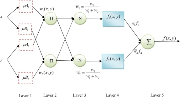
are the output function parameters [26].The architecture of ANFIS is presented in Figure 4. It includes five layers; all are fixed nodes, except the first and fourth nodes, which are adaptive nodes.
100000 110000 120000 130000 140000 150000 160000 170000 180000 190000
Jan Feb Mar Apr May Jun Jul Aug Sep Oct Nov Dec
Pr ec ip it at ion ( m m ) Month
Figure 3.Average power generation in the Dez hydropower plant. Table 1.Presenting the datasets and the statistical characteristics.
Parameter Mode Mean Min S.D. First
Quartile Median
Third
Quartile Max Skew. Kurtosis. Ht 26,545.98 165,297.70 26,545.98 56,093.06 130,338.42 168,568.96 203,734.07 354,879.53 −0.10 2.76 Qt 63.28 651.71 63.28 615.23 209.87 430.22 842.41 3643.84 1.86 6.91
Pt 0.00 42.82 0.00 46.91 0.47 27.97 71.81 238.47 1.10 3.69
Ht: Hydroelectric Energy (MWH) at month t; Qt: River Inflow (m3/s) at month t; Pt: precipitation (mm) at month t;
S.D.: Standard Deviation.
2.2. ANFIS: Adaptive Neuro-Fuzzy Inference System
Jang (1993) [22] developed ANFIS as a joint of artificial neural network and the fuzzy inference system [23]. The learning ability of artificial neural networks (ANN) and the fuzzy reasoning create a valuable capability to fit a relationship between input and output spaces [24]. On the other hand, the ANFIS uses the training capability of ANN to assign and adjust the membership functions. The back-propagation algorithm enables the model to adjust the parameters until an acceptable error is reached [25]. Suppose that the system of fuzzy inference include x & y as inputs and z as output. Two if-then rules could be utilized for Sugeno model as follows:
Rule one: ifxand y =A1andB1, respectively, then f1=p1x+q1y+r1.
Rule two: ifxandy=A2andB2, respectively, then f2=p2x+q2y+r2
whereA1,B1,A2,B2are considered as the labels of linguistic. Furthermore,p1,p2,q1,q2,r1andr2are
the output function parameters [26].
The architecture of ANFIS is presented in Figure4. It includes five layers; all are fixed nodes, except the first and fourth nodes, which are adaptive nodes.
Figure 4.Architecture of adaptive neuro-fuzzy inference system in this study.
Layer 1: The nodes act adaptive in generating the membership grades of the inputs [24]: O1,i=µAi(x), fori = 1, 2, or
O1,i =µBi−2(y), fori = 3, 4.
(1) It should be noted thatiis the number of inputs andO1,i toO5,i are the output of each layer.
Several memberships could be used for this purpose; among all Gaussian functions presented in the Equation (1), the following was utilized in this study:
µ(x) =exp " −0.5 x−ci σi 2# (2) whereciandσiare set parameters with maximum and minimum of one and zero, respectively [22].
Layer 2: this layer is a rule node with AND/OR operator to get an output which called firing strengthsO2,i:
O2,i =µAi(x)µBi(y), i = 1, 2 (3)
Layer 3: presents an average node computing the normalized firing strength as follows: O3,i =wi = wi
w1+w2, i
= 1, 2 (4)
Layer 4: this layer contains the consequent nodes for which thep,qandrparameters were tuned during the learning process:
O4,i=wifi=wi(pix+qiy+ri) (5)
Layer 5: this layer contains the output nodes which compute the total average of output through a sum of entire input signals [27]:
O5,i= f =
∑
iwifi (6)
While the ANFIS has high capability to map the input to the output as a black-box model, it suffers from a long training time to assign the proper values to the parameters of membership function. To overcome this problem we use the optimization algorithm of grey wolf.
2.3. Grey Wolf Optimization (GWO)
The optimization algorithm of Grey wolf known as GWO is known as an advanced meta-heuristic nature-inspired for an efficient optimization [28]. This algorithm was developed through imitating the foraging behavior of grey wolfs performing in groups of five-12 individuals which are at the top of food chain [29]. Grey wolves follow a social hierarchy strictly.
The leaders include a couple of female and male, called alpha (α), who are in charge of decision
making while hunting, resting and so on. Beta (β) is the next level helping alpha in making decisions,
while they should obey the alpha. The beta wolves can be male and female and the role of them is disciplining the group. They are the best candidate for substituting the alpha when they become older or die. The next level is called delta (δ) and play the role of scouts, sentinels, hunters and so on. The last
level is called omega (ω), which are the weakest level. They act as babysitters. While this level is the
weakest, without omega wolves, internal fights may be observed in the group. Hunting, along with the social hierarchy, is a major social behavior of grey wolves. Muro et al. [30] expressed the three steps in the grey wolves hunting:
1. Identifying, following and approaching the prey; 2. Encircling the prey;
3. Attacking the prey.
These two social behaviors are considered in the GWO algorithm [29]. In mathematical modeling of the algorithm, αis considered as the fittest solution, and in the next steps, β, δand ω. The mathematical formulation of encircling could be presented as follows [28]:
→ D= → C·→Xp(t)−X(t) (7) → X(t+1) = → Xp(t)− → A·→D (8) where, → Aand →
Cwould work as the vectors of the coefficient. Furthermore,
→
Xpwould determine the
positions of prey and→Xis the wolf's positions. Here,→Dwould be the vector for specifying a new position of the GW andtis the iteration time. The
→ Cand → Aformulated as [28]: → A=2→a·→r1− → a (9) → C=2·→r2 (10)
where→a presents the set of vectors over the iteration that change in value from 2 to 0 linearly. The→r1
and→r2represent random vectors in[0, 1].
Theα leads the hunting, whileβ andδcontribute in this task occasionally. For mathematical
representation of hunting, it was assumed that the alpha, bata and delta include better knowledge on the prey’s locations. Thus, the optimal solutions for the three positions can be registered. Consequently, the rest of the wolves will follow and update their postions accordingly.
→ Dα= → C1· → Xα− → X (11) → Dβ= → C2· → Xβ− → X (12) → Dδ= → C3· → Xδ−→X (13) → X1= → Xα−A1· → Dα (14)
→ X2= → Xβ−A2· → Dβ (15) → X3= → Xδ−A3· → Dδ (16) → X(t+1) = → X1+ → X2+ → X3 3 (17)
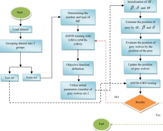
When the prey stops, the grey wolves start to attack. The vectorAis a random value in the interval[−2a, 2a]. The|A|<1 leads to grey wolves’ attack while|A|>1 force them to move away to find a better solution. Figure5shows the framework of the GWO algorithm.
Figure 5.The flowchart of ANFIS-GWO modeling. 2.4. Performance Criteria
The assessment of the proposed model’s efficiencies, including accuracy and agreement, was evaluated using statistical criteria, such as the confidence index (CI), root mean square error (RMSE), Nash-Sutcliffe Efficiency (NSE), coefficient of determination (R2), index of agreement (d), relative absolute error (RAE) and mean absolute error (MAE).
The evaluation criteria of RMSE and MAE are common mean error indicators that indicated how close data points are to a best fit line (Equations (18) & (19)) [31].
According to Nash and Sutcliffe [32], the NSE is defined as the sum of the absolute squared differences of the observed and estimated data normalized by the variance minus one. (Equation (21)). As determined by [33], the range of NSE is from one to−∞. When NSE is less than 0, the mean observed value have been a better predictor than the model. It describes the plot of observed data versus estimated data, and how well they fit the 1:1 line.
Furthermore, according to Bravais-Pearson, the R2presents the squared value of the correlation coefficient describing how much of the observed dispersion is delivered by the prediction. The value of R2may vary from 1 and 0. The 0, and 1 values would present no correlation between observed and
predicted data, and dispersion of the estimation data is equal to that of the observation, respectively [33] (Equation (20)).
The index of agreement d [34] prevail over the insensitivity of NSE and R2to differences in the means and variances of the observed and estimated data [35]. The index of agreement demonstrates the ratio of the mean square error and the potential error [36] (Equation (22)). The range of d similar to R2changes from 0 for the no correlation to 1, which is a perfect fit.
The RAE is a non-negative index that indicates a ratio of the overall agreement level between observed and estimated datasets. The range of RAE may change from 0 for a perfect fit to ∞, which means no upper bound. The Confidence index (CI) is the product of NSE and d, which ranges between 1 (perfect fit) and−∞. Lower than zero values means that the mean observed values have been a better predictor than the model.
The evaluation criteria were calculated based on the following equations: RMSE= r 1 N N
∑
i=1 (Oi−Pi)2, 0≤RMSE<∞ (18) MAE= 1 N N∑
i=1 |Oi−Pi|, 0≤MAE<∞ (19) R2= ∑N i=1 Oi−O Pi−P r ∑N i=1 Oi−O 2q ∑N i=1 Pi−P 2 2 , 0≤r2≤1 (20) NSE=1− ∑ N i=1(Oi−Pi)2 ∑N i=1 Oi−O 2, −∞< NSE≤1 (21) d=1− ∑ N i=1(Pi−Oi)2 ∑N i=1 Pi−O + Oi−O 2, 0≤d≤1 (22) PI =1− ∑ N i=1(Oi−Pi)2 ∑N i=1(Oi−Oi−1)2 , −∞<PI <∞ (23) CI =d×NSE, −∞≤CI ≤1 (24) RAE= ∑ N i=1|Oi−Pi| ∑N i=1 Oi−O (25) In which theOi is observation value, Pi is the predicted model output, O¯ is the average ofobservations,Pis the average of model outputs andNis number of data. 3. Results
In this study, the inflow of the Dez dam and the average precipitation over the whole basin were utilized to forecast the hydropower generation. For this purpose, the time series divided into two subsets as the train and test subsets. 70% of data was assigned as the train and the remaining 30% for test phase.
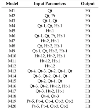
Different input combinations were evaluated and used in the modeling process. The final selection of input combinations was based on the correlation analysis of variables in Table 3, the physical nature of variables and applicability of models presented in Table2. Based on the availability of different measured parameters in the dam, one can choose which model is applicable for prediction of hydropower, and these different combinations strengthen the applicability of model in different data availability of the study. Some models were only based on inflow to the dam and rainfall such as: M1, M2, M3, M13, M14, M15, M18, M19 and M20. These models did not require the hydropower
generation of the dam in previous time steps and, based on inflow and precipitation, can predict the hydropower generation in the plan. Some models used lagged values of hydropower generation of the dam in previous time steps as input vectors and these models did not require further information of inflow or precipitation in prediction of hydropower generation. These models, such as M5, M7 M10, M11 and M12, are lagged based models. The other models are based on combination of lagged values of hydropower generation, inflow and precipitation, such as M4, M6, M8, M9, M16 and M17.
Table 2.Different input combination used for ANFIS and GWO-ANFIS modeling.
Model Input Parameters Output
M1 Qt Ht M2 Qt, Pt Ht M3 Qt-1, Qt Ht M4 Qt-1, Qt, Ht-1 Ht M5 Ht-1 Ht M6 Qt-1, Qt, Pt, Ht-1 Ht M7 Ht-2, Ht-1 Ht M8 Qt, Ht-2, Ht-1 Ht M9 Qt-1, Qt, Ht-2, Ht-1 Ht M10 Ht-12, Ht-2, Ht-1 Ht M11 Ht-12, Ht-1 Ht M12 Ht-12 Ht M13 Qt-4, Qt-3, Qt-2, Qt-1, Qt Ht M14 Qt-3, Qt-2, Qt-1, Qt Ht M15 Qt-2, Qt-1, Qt Ht M16 Qt-3, Qt-2, Ht-12, Ht-1 Ht M17 Qt-3, Ht-2, Ht-1 Ht M18 Qt-4, Qt-3 Ht M19 Pt-5, Pt-4, Qt-4, Qt-3, Qt-2 Ht M20 Pt-5, Pt-4, Qt-3, Qt-2 Ht
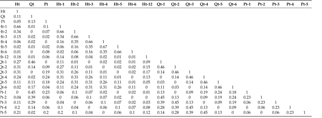
According to Table2, the discharge, precipitation, and the hydropower generation with different lags were used to forecast the hydropower generation for the next month. The correlation coefficients between the input variables were calculated and are presented in Table3; they oscillate between 0.01 and 0.67. It should be noted that Q is the inflow of the dam, but not the inflow of the turbine. Therefore, as the Dam is multipurpose, and the water stored in the dam is also used for irrigation, it is possible to use Qtto predict the Ht. All 20 input combinations were used for modeling by ANFIS and
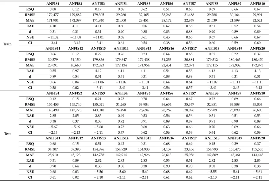
GWO-ANFIS to evaluate the capability of GWO in optimizing the ANFIS parameters, which shows better performance. The results of ANFIS modeling are presented in Table4. Among the different input combinations, the first three models were not capable to reproduce satisfying results. Negative values were assigned to the NSE and CI, which show the poor application of models. The same procedure is visible in M13, M14, M15, M18, M19 and M20. However, the M4 to M11, M16 and M17 performed well. Among these combinations, M4 is the best and M8, M10 and M9 are the next in row. It should be noted that although the M4 was the best based on the evaluation criteria, according to Table2, M17 was selected as the best model. This was because all the inputs of M17, i.e., Qt-3, Ht-2 and Ht-1, have at least a one-month lag. In addition, the results of M4 and M17 were not considerably different. This pattern was repeated for the test phase. Consequently, it can be concluded that, ANFIS was capable to forecast the hydropower generation satisfactorily.
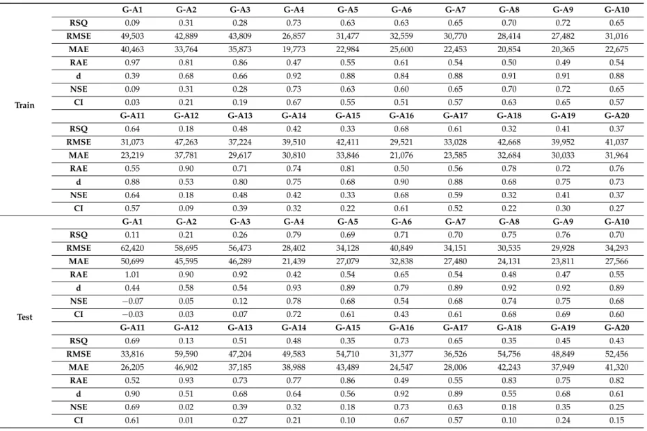
In the next step, the coupled model of GWO-ANFIS was utilized for hydropower generation forecasting. Results are presented in Table5. According to Table5, the model performed well in all input combinations. As the d, NSE and CI values were positive in all the models, the new modeling technique of GWO-ANFIS provided a superior capability in forecasting hydropower generation, while the ANFIS results failed in nine models. In addition, based on the evaluation criteria, the accuracy of forecasting was higher for GWO-ANFIS.
Table 3.Correlation coefficients between parameters. Ht Qt Pt Ht-1 Ht-2 Ht-3 Ht-4 Ht-5 Ht-6 Ht-12 Qt-1 Qt-2 Qt-3 Qt-4 Qt-5 Qt-6 Pt-1 Pt-2 Pt-3 Pt-4 Pt-5 Ht 1 Qt 0.11 1 Pt 0.05 0.13 1 Ht-1 0.66 0.01 0.1 1 Ht-2 0.34 0 0.07 0.66 1 Ht-3 0.15 0.02 0.02 0.34 0.66 1 Ht-4 0.06 0.02 0 0.16 0.35 0.66 1 Ht-5 0.02 0.01 0.02 0.06 0.16 0.35 0.67 1 Ht-6 0.01 0 0.08 0.02 0.06 0.16 0.35 0.66 1 Ht-12 0.18 0.01 0.06 0.14 0.08 0.04 0.02 0.01 0.01 1 Qt-1 0.27 0.46 0 0.11 0.01 0 0.02 0.02 0.01 0.09 1 Qt-2 0.31 0.14 0.09 0.27 0.11 0.01 0 0.02 0.02 0.15 0.46 1 Qt-3 0.31 0 0.19 0.31 0.26 0.11 0.01 0 0.02 0.17 0.14 0.46 1 Qt-4 0.24 0.02 0.24 0.31 0.31 0.26 0.11 0.01 0 0.13 0 0.14 0.46 1 Qt-5 0.11 0.11 0.18 0.24 0.31 0.31 0.26 0.11 0.01 0.05 0.03 0 0.14 0.46 1 Qt-6 0.02 0.17 0.04 0.11 0.24 0.31 0.31 0.26 0.11 0 0.11 0.03 0 0.14 0.46 1 Pt-1 0 0.45 0.23 0.06 0.1 0.07 0.02 0 0.02 0.01 0.13 0 0.09 0.19 0.24 0.18 1 Pt-2 0.04 0.39 0.06 0 0.06 0.1 0.07 0.02 0 0 0.45 0.13 0 0.09 0.19 0.24 0.23 1 Pt-3 0.11 0.29 0 0.04 0 0.06 0.1 0.07 0.02 0.03 0.39 0.45 0.13 0 0.09 0.19 0.06 0.23 1 Pt-4 0.2 0.14 0.06 0.1 0.04 0 0.06 0.1 0.07 0.08 0.28 0.39 0.45 0.13 0 0.09 0 0.06 0.23 1 Pt-5 0.21 0.02 0.2 0.2 0.1 0.04 0 0.06 0.1 0.12 0.14 0.28 0.39 0.45 0.13 0 0.06 0 0.06 0.23 1
Table 4.Results of ANFIS modeling in train and test phases.
Train
ANFIS1 ANFIS2 ANFIS3 ANFIS4 ANFIS5 ANFIS6 ANFIS7 ANFIS8 ANFIS9 ANFIS10
RSQ 0.08 0.12 0.17 0.68 0.62 0.51 0.63 0.69 0.66 0.67 RMSE 179,477 179,882 179,305 29,260 32,165 38,263 31,488 29,768 30,164 29,991 MAE 171,981 172,397 171,840 21,000 23,451 28,172 22,869 21,539 21,599 22,521 RAE 4.10 4.11 4.11 0.50 0.56 0.67 0.55 0.51 0.52 0.54 d 0.31 0.31 0.31 0.90 0.88 0.83 0.88 0.90 0.89 0.89 NSE −11.02 −11.08 −11.01 0.68 0.61 0.45 0.63 0.67 0.66 0.67 CI −3.41 −3.42 −3.41 0.61 0.54 0.38 0.56 0.60 0.59 0.60
ANFIS11 ANFIS12 ANFIS13 ANFIS14 ANFIS15 ANFIS16 ANFIS17 ANFIS18 ANFIS19 ANFIS20
RSQ 0.66 0.12 0.22 0.26 0.23 0.64 0.65 0.35 0.22 0.32 RMSE 30,579 51,150 179,856 179,647 179,438 31,253 30,884 179,512 180,465 180,470 MAE 23,091 40,660 172,323 172,134 171,954 22,451 22,071 172,115 172,932 172,973 RAE 0.55 0.97 4.12 4.11 4.11 0.54 0.53 4.12 4.13 4.13 d 0.89 0.54 0.31 0.31 0.31 0.88 0.89 0.31 0.31 0.31 NSE 0.66 0.04 −11.06 −11.02 −11.01 0.64 0.64 −11.02 −11.11 −11.11 CI 0.58 0.02 −3.41 −3.41 −3.41 0.56 0.57 −3.41 −3.43 −3.43 Test
ANFIS1 ANFIS2 ANFIS3 ANFIS4 ANFIS5 ANFIS6 ANFIS7 ANFIS8 ANFIS9 ANFIS10
RSQ 0.12 0.15 0.21 0.73 0.70 0.64 0.67 0.72 0.69 0.66 RMSE 155,453 155,740 155,021 31,265 33,984 36,654 35,367 32,951 33,508 35,003 MAE 143,490 143,773 143,018 24,498 26,694 28,267 28,096 25,989 25,890 26,600 RAE 2.85 2.85 2.83 0.49 0.53 0.56 0.56 0.51 0.51 0.53 d 0.38 0.37 0.38 0.92 0.91 0.89 0.89 0.91 0.90 0.89 NSE −5.67 −5.69 −5.60 0.73 0.68 0.63 0.66 0.70 0.69 0.66 CI −2.13 −2.13 −2.11 0.67 0.62 0.56 0.59 0.64 0.62 0.59
ANFIS11 ANFIS12 ANFIS13 ANFIS14 ANFIS15 ANFIS16 ANFIS17 ANFIS18 ANFIS19 ANFIS20
RSQ 0.68 0.15 0.51 0.42 0.31 0.68 0.69 0.45 0.39 0.37 RMSE 34,307 59,395 154,896 154,929 154,933 34,157 33,456 154,793 155,475 155,535 MAE 25,910 45,123 142,788 142,914 142,926 26,613 25,956 142,809 143,361 143,448 RAE 0.51 0.89 2.82 2.83 2.83 0.53 0.51 2.82 2.83 2.83 d 0.90 0.64 0.38 0.38 0.38 0.90 0.90 0.38 0.38 0.38 NSE 0.68 0.03 −5.56 −5.60 −5.60 0.68 0.69 −5.55 −5.61 −5.61 CI 0.61 0.02 −2.10 −2.11 −2.11 0.61 0.62 −2.10 −2.11 −2.11
Table 5.Results of GWO-ANFIS modeling in train and test phases. G-A is the abbreviation of GWO-ANFIS.
Train
G-A1 G-A2 G-A3 G-A4 G-A5 G-A6 G-A7 G-A8 G-A9 G-A10
RSQ 0.09 0.31 0.28 0.73 0.63 0.63 0.65 0.70 0.72 0.65 RMSE 49,503 42,889 43,809 26,857 31,477 32,559 30,770 28,414 27,482 31,016 MAE 40,463 33,764 35,873 19,773 22,984 25,600 22,453 20,854 20,365 22,675 RAE 0.97 0.81 0.86 0.47 0.55 0.61 0.54 0.50 0.49 0.54 d 0.39 0.68 0.66 0.92 0.88 0.84 0.88 0.91 0.91 0.88 NSE 0.09 0.31 0.28 0.73 0.63 0.60 0.65 0.70 0.72 0.65 CI 0.03 0.21 0.19 0.67 0.55 0.51 0.57 0.63 0.65 0.57
G-A11 G-A12 G-A13 G-A14 G-A15 G-A16 G-A17 G-A18 G-A19 G-A20
RSQ 0.64 0.18 0.48 0.42 0.33 0.68 0.61 0.32 0.41 0.37 RMSE 31,073 47,263 37,224 39,510 42,411 29,521 33,028 42,668 39,952 41,037 MAE 23,219 37,781 29,617 30,810 33,846 21,076 23,585 32,684 30,033 31,964 RAE 0.55 0.90 0.71 0.74 0.81 0.50 0.56 0.78 0.72 0.76 d 0.88 0.53 0.80 0.75 0.68 0.90 0.88 0.68 0.75 0.73 NSE 0.64 0.18 0.48 0.42 0.33 0.68 0.59 0.32 0.41 0.37 CI 0.57 0.09 0.39 0.32 0.22 0.61 0.52 0.22 0.30 0.27 Test
G-A1 G-A2 G-A3 G-A4 G-A5 G-A6 G-A7 G-A8 G-A9 G-A10
RSQ 0.11 0.21 0.26 0.79 0.69 0.71 0.70 0.75 0.76 0.70 RMSE 62,420 58,695 56,473 28,402 34,128 40,849 34,151 30,535 29,928 34,293 MAE 50,699 45,595 46,289 21,439 27,079 32,838 27,480 24,131 23,811 27,566 RAE 1.01 0.90 0.92 0.42 0.54 0.65 0.54 0.48 0.47 0.55 d 0.44 0.58 0.54 0.93 0.89 0.79 0.89 0.92 0.92 0.89 NSE −0.07 0.05 0.12 0.78 0.68 0.54 0.68 0.74 0.75 0.68 CI −0.03 0.03 0.07 0.72 0.61 0.43 0.61 0.68 0.69 0.60
G-A11 G-A12 G-A13 G-A14 G-A15 G-A16 G-A17 G-A18 G-A19 G-A20
RSQ 0.69 0.13 0.51 0.48 0.35 0.73 0.65 0.35 0.45 0.43 RMSE 33,816 59,590 47,204 49,583 54,710 31,377 36,526 54,756 48,849 52,456 MAE 26,205 46,902 37,185 38,988 43,489 24,547 28,006 42,243 37,949 41,320 RAE 0.52 0.93 0.73 0.77 0.86 0.49 0.55 0.83 0.75 0.82 d 0.90 0.51 0.68 0.64 0.56 0.92 0.89 0.55 0.68 0.61 NSE 0.69 0.02 0.39 0.32 0.18 0.73 0.63 0.18 0.35 0.25 CI 0.61 0.01 0.27 0.21 0.10 0.67 0.57 0.10 0.24 0.15
Energies 2019, 12, 289 4 of 20
M4 M10
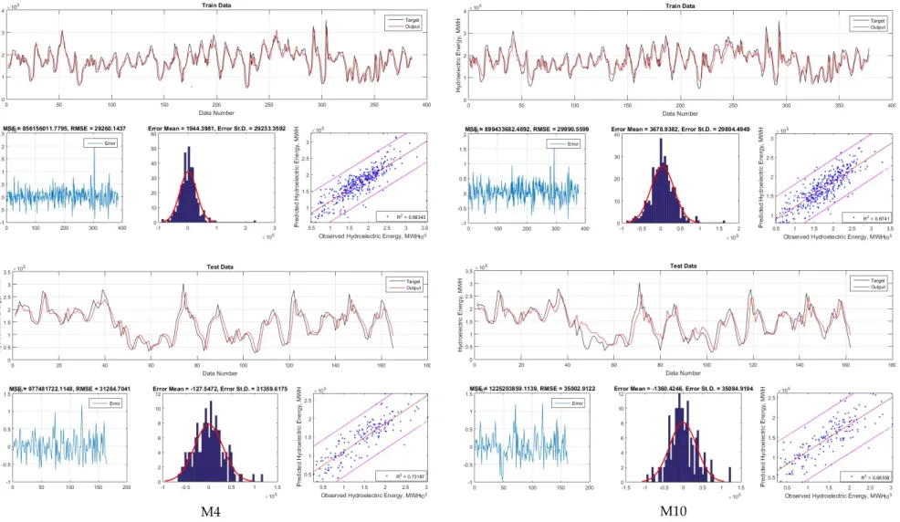
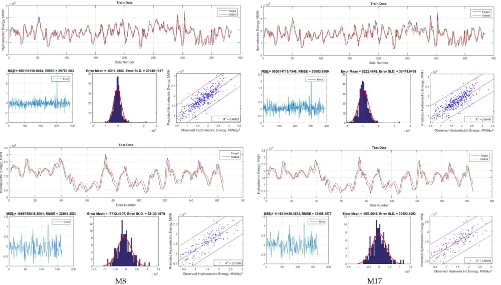
M8 M17 Figure 6. Observed and forecasted time series of hydropower generation using ANFIS. Figure 6.Observed and forecasted time series of hydropower generation using ANFIS.
M4 M10
M8 M17
Figure 7. Observed and forecasted time series of hydropower generation using GWO-ANFIS. Figure 7.Observed and forecasted time series of hydropower generation using GWO-ANFIS.
The time series of observed and forecasted hydropower in train and test phases for M4, M8, M10 and M117 are presented in Figures6and7. Both ANFIS and GWO-ANFIS performed well, while the GWO-ANFIS was superior due to less error. In addition, it can be observed that the M4 and M10 presented better input combinations, while for dam operation and reservoir management, M17 was more practical.
Although Figures6and7and Tables4and5show the observed and forecasted values and evaluation criteria for all models, the error distribution among models could not be discussed via these figures and tables. Therefore, the box plot of error during the train and test phases was plotted in Figure8. In Figure8, it can be observed that the GWO-ANFIS was superior to the ANFIS considerably in almost all input combinations. Nevertheless, the error of ANFIS in nine models was considerably higher than the GWO-ANFIS.Energies 2019, 12, 289 1 of 20
Figure 8. Box plot of errors for ANFIS and GWO-ANFIS modeling in training and testing phases. F
and G refer to ANFIS and GWO-ANFIS, respectively.
The meta-heuristic optimization algorithm of GWO-ANFIS showed an acceptable efficiency in the optimization of the unknown parameters in ANFIS. Although the number of optimization parameters in ANFIS and GWO-ANFIS was the same, the main complexity quantifier was the number of unknown parameters to be tuned for model training. The present research sought to ensure that the numerical complexity of the two modeling approaches was similar. Furthermore, the ANFIS models required the derivative calculation for unknown parameters, which increased the computational time and space necessary for training. While the GWO-ANFIS models did not need the derivative calculation, this would lead to less computation and faster convergence.
4. Conclusions
In this study, a coupled of adaptive neuro-fuzzy inference system and grey wolf optimization was utilized for one month ahead hydropower generation. For this purpose, 53 years of monthly data of inflow to the dam reservoir and the hydropower generation were used. Twenty input-output combinations were considered to evaluate the model robustness and to find the best input-output combination. Based on the results, GWO was capable to improve the ANFIS performance
Figure 8.Box plot of errors for ANFIS and GWO-ANFIS modeling in training and testing phases. F and G refer to ANFIS and GWO-ANFIS, respectively.
The meta-heuristic optimization algorithm of GWO-ANFIS showed an acceptable efficiency in the optimization of the unknown parameters in ANFIS. Although the number of optimization parameters in ANFIS and GWO-ANFIS was the same, the main complexity quantifier was the number of unknown
parameters to be tuned for model training. The present research sought to ensure that the numerical complexity of the two modeling approaches was similar. Furthermore, the ANFIS models required the derivative calculation for unknown parameters, which increased the computational time and space necessary for training. While the GWO-ANFIS models did not need the derivative calculation, this would lead to less computation and faster convergence.
4. Conclusions
In this study, a coupled of adaptive neuro-fuzzy inference system and grey wolf optimization was utilized for one month ahead hydropower generation. For this purpose, 53 years of monthly data of inflow to the dam reservoir and the hydropower generation were used. Twenty input-output combinations were considered to evaluate the model robustness and to find the best input-output combination. Based on the results, GWO was capable to improve the ANFIS performance considerably. GWO-ANFIS performed well in all 20 combinations based on the evaluation criteria while the ANFIS failed in nine out of 20 combinations. Additionally, the box plot of error in all combinations shows the superiority of GWO-ANFIS. Overall, it can be concluded that, GWO-ANFIS is capable to forecast the hydropower generation satisfactorily, which makes it a suitable tool for policymakers. Furthermore, for the future research direction, it is important to mention that, not all the rules in the model architecture are essential; thus, it is necessary to reduce trained models complexity through eliminating the noncontributing rules which leads to the reduction of network’s computational cost. To improve the proposed method, utilizing the other optimization algorithms for creating novel hybrid prediction models, as well as applying ensemble models in this application is suggested for the future research. In fact, the potential of ensemble machine learning models have not yet been fully explored in the prediction of hydropower generation, which leaves great room for future investigations. In addition, a limitation of our proposed model was that while the effective factors for which the model was implemented were the most critical factors, there may be other relevant factors that should be used. For instance, climate change and drought variations need to be separated from the general trend of the data set. Therefore, the addition of these concepts is left for future work.
Author Contributions:Conceptualization, M.D., H.R.-M. and F.H.; Data curation, M.D., H.R.-M. and F.H.; Formal analysis, M.D., A.M., H.R.-M. and F.H.; Methodology, M.D., H.R.-M., S.S. and F.H.; Resources, H.R.-M. and F.H.; Software, H.R.-M., M.D. and F.H.; Supervision, K.-w.C. and E.K.Z.; Visualization, F.H., A.M., S.S. and K.-w.C.; Writing—original draft, M.D., H.R.-M., F.H. and A.M.; Writing—review & editing, M.D., H.R.-M., F.H., A.M., S.S. and K.-w.C.
Conflicts of Interest:The authors declare no conflict of interest. References
1. Hamlet, A.F.; Huppert, D.; Lettenmaier, D.P. Economic value of long-lead streamflow forecasts for Columbia River hydropower.J. Water Resour. Plan. Manag.2002,1282, 91–101. [CrossRef]
2. Tang, G.L.; Zhou, H.C.; Li, N.; Wang, F.; Wang, Y.; Jian, D. Value of medium-range precipitation forecasts in inflow prediction and hydropower optimization.Water Resour. Manag.2010,24, 2721–2742. [CrossRef] 3. Zhou, H.; Tang, G.; Li, N.; Wang, F.; Wang, Y.; Jian, D. Evaluation of precipitation forecasts from NOAA
global forecast system in hydropower operation.J. Hydroinform.2011,13, 81–95. [CrossRef]
4. Block, P. Tailoring seasonal climate forecasts for hydropower operations.Hydrol. Earth Syst. Sci.2011,15, 1355–1368. [CrossRef]
5. Rheinheimer, D.E.; Bales, R.C.; Oroza, C.A.; Lund, J.R.; Viers, J.H. Valuing year-to-go hydrologic forecast improvements for a peaking hydropower system in the Sierra Nevada.Water Resour. Res.2016,52, 3815–3828. [CrossRef]
6. Zhang, X.; Peng, Y.; Xu, W.; Wang, B. An Optimal Operation Model for Hydropower Stations Considering Inflow Forecasts with Different Lead-Times.Water Resour. Manag.2017. [CrossRef]
7. Peng, Y.; Xu, W.; Liu, B. Considering precipitation forecasts for real-time decision-making in hydropower operations.Int. J. Water Resour. Dev.2017,33, 987–1002. [CrossRef]
8. Jiang, Z.; Li, R.; Li, A.; Ji, C. Runoff forecast uncertainty considered load adjustment model of cascade hydropower stations and its application.Energy2018,158, 693–708. [CrossRef]
9. Mosavi, A.; Ozturk, P.; Chau, K.W. Flood prediction using machine learning models: Literature review.Water
2018,10, 1536. [CrossRef]
10. Hammid, A.T.; Sulaiman, M.H.B.; Abdalla, A.N. Prediction of small hydropower plant power production in Himreen Lake dam (HLD) using artificial neural network.Alexandria Eng. J.2018,57, 211–221. [CrossRef] 11. Boucher, M.A.; Ramos, M.H. Ensemble Streamflow Forecasts for Hydropower Systems.Handb. Hydrometeorol.
Ensemble Forecast.2018, 1–19. [CrossRef]
12. Choubin, B.; Moradi, E.; Golshan, M.; Adamowski, J.; Sajedi-Hosseini, F.; Mosavi, A. An Ensemble prediction of flood susceptibility using multivariate discriminant analysis, classification and regression trees, and support vector machines.Sci. Total Environ.2019,651, 2087–2096. [CrossRef] [PubMed]
13. Shamshirband, S.; Jafari Nodoushan, E.; Adolf, J.E.; Abdul Manaf, A.; Mosavi, A.; Chau, K.W. Ensemble models with uncertainty analysis for multi-day ahead forecasting of chlorophyll a concentration in coastal waters.Eng. Appl. Comput. Fluid Mech.2019,13, 91–101. [CrossRef]
14. Bui, K.T.T.; Bui, D.T.; Zou, J.; Van Doan, C.; Revhaug, I. A novel hybrid artificial intelligent approach based on neural fuzzy inference model and particle swarm optimization for horizontal displacement modeling of hydropower dam.Neural Comput. Appl.2018,29, 1495–1506.
15. Kim, Y.O.; Eum, H.I.; Lee, E.G.; Ko, I.H. Optimizing Operational Policies of a Korean Multireservoir System Using Sampling Stochastic Dynamic Programming with Ensemble Streamflow Prediction.J. Water Resour. Plan Manag.2007,133, 4. [CrossRef]
16. Ch, S.; Anand, N.; Panigrahi, B.K. Streamflow forecasting by SVM with quantum behaved particle swarm optimization.Neurocomputing2013,101, 18–23. [CrossRef]
17. Cote, P.; Leconte, R. Comparison of Stochastic Optimization Algorithms for Hydropower Reservoir Operation with Ensemble Streamflow Prediction.J. Water Resour. Plan Manag.2016,142, 04015046. [CrossRef] 18. Keshtegar, B.; Falah Allawi, M.; Afan, H.A.; El-Shafie, A. Optimized River Stream-Flow Forecasting Model
Utilizing High-Order Response Surface Method.Water Resour. Manag.2016,30, 3899–3914. [CrossRef] 19. Paul, M.; Negahban-Azar, M. Sensitivity and uncertainty analysis for streamflow prediction using multiple
optimization algorithms and objective functions: San Joaquin Watershed, California. Model. Earth Syst. Environ.2018,4, 1509–1525. [CrossRef]
20. Karballaeezadeh, N.; Mohammadzadeh, D.; Shamshirband, S.; Hajikhodaverdikhan, P.; Mosavi, A.; Chau, K.W. Prediction of remaining service life of pavement using an optimized support vector machine.
Eng. Appl. Comput. Fluid Mech.2019,16, 120–144.
21. Niu, M.; Wang, Y.; Sun, S.; Li, Y. A novel hybrid decomposition-and-ensemble model based on CEEMD and GWO for short-term PM2.5 concentration forecasting.Atmos. Environ.2016,134, 168–180. [CrossRef] 22. Jang, J.-S.R. ANFIS: Adaptive-network-based fuzzy inference system.IEEE Trans. Syst. Man Cybern.1993,23,
665–685. [CrossRef]
23. Choubin, B.; Khalighi-Sigaroodi, S.; Malekian, A.; Ki¸si, O. Multiple linear regression, multi-layer perceptron network and adaptive neuro-fuzzy inference system for the prediction of precipitation based on large-scale climate signals.Hydrol. Sci. J.2016,61, 1001–1009. [CrossRef]
24. Firat, M.; Güngör, M. Hydrological time-series modelling using an adaptive neuro-fuzzy inference system.
Hydrol. Process.2007,22, 2122–2132. [CrossRef]
25. Shabri, A. A Hybrid Wavelet Analysis and Adaptive Neuro-Fuzzy Inference System for Drought Forecasting.
Appl. Math. Sci.2014,8, 6909–6918. [CrossRef]
26. Kisi, O.; Shiri, J. Precipitation forecasting using wavelet genetic programming and wavelet-neuro-fuzzy conjunction models.Water Resour. Manag.2011,25, 3135–3152. [CrossRef]
27. Awan, J.A.; Bae, D.H. Drought prediction over the East Asian monsoon region using the adaptive neuro-fuzzy inference system and the global sea surface temperature anomalies. Int. J. Climatol. 2016,36, 4767–4777. [CrossRef]
28. Mirjalili, S.; Mirjalili, S.M.; Lewis, A. Grey wolf optimizer.Adv. Eng. Softw.2014,69, 46–61. [CrossRef] 29. Bozorg-Haddad, O.Advanced Optimization by Nature-Inspired Algorithms; Springer: Singapore, 2017. 30. Muro, C.; Escobedo, R.; Spector, L.; Coppinger, R. Wolf-pack (Canis Lupus) hunting strategies emerge from
31. Amr, H.; El-Shafie, A.; El Mazoghi, H.; Shehata, A.; Taha, M.R. Artificial neural network technique for rainfall forecasting applied to Alexandria, Egypt.Int. J. Phys. Sci.2011,6, 1306–1316.
32. Nash, J.E.; Sutcliffe, J.V. River flow forecasting through conceptual models part I—A discussion of principles.
J. Hydrol.1970,10, 282–290. [CrossRef]
33. Krause, P.; Boyle, D.P.; Bäse, F. Comparison of different efficiency criteria for hydrological model assessment.
Adv. Geosci.2005,5, 89–97. [CrossRef]
34. Willmott, C.J. On the validation of models.Phys. Geogr.1981,2, 184–194. [CrossRef]
35. Legates, D.R.; McCabe, G.J. Evaluating the use of “goodness-of-fit” measures in hydrologic and hydroclimatic model validation.Water Resour. Res.1999,35, 233–241. [CrossRef]
36. Willmott, C.J. On the evaluation of model performance in physical geography. InSpatial Statistics and Models; Springer: Dordrecht, The Netherlands, 1984; pp. 443–460.
© 2019 by the authors. Licensee MDPI, Basel, Switzerland. This article is an open access article distributed under the terms and conditions of the Creative Commons Attribution (CC BY) license (http://creativecommons.org/licenses/by/4.0/).