This is an Open Access document downloaded from ORCA, Cardiff University's institutional
repository: http://orca.cf.ac.uk/72823/
This is the author’s version of a work that was submitted to / accepted for publication.
Citation for final published version:
Smallman, Luke and Artemiou, Andreas 2017. A study on imbalance support vector machine
algorithms for sufficient dimension reduction. Communications in Statistics - Theory and Methods
46 (6) , pp. 2751-2763. 10.1080/03610926.2015.1048889 file
Publishers page: http://dx.doi.org/10.1080/03610926.2015.1048889
<http://dx.doi.org/10.1080/03610926.2015.1048889>
Please note:
Changes made as a result of publishing processes such as copy-editing, formatting and page
numbers may not be reflected in this version. For the definitive version of this publication, please
refer to the published source. You are advised to consult the publisher’s version if you wish to cite
this paper.
This version is being made available in accordance with publisher policies. See
http://orca.cf.ac.uk/policies.html for usage policies. Copyright and moral rights for publications
made available in ORCA are retained by the copyright holders.
A Study on Imbalance Support Vector Machine
Algorithms for Sufficient Dimension Reduction
Luke Smallman and Andreas Artemiou School of Mathematics, Cardiff University
Abstract
Li, Artemiou and Li (2011) presented the novel idea of using Support Vector Machines to perform sufficient dimension reduction. In this work, we investigate the potential improvement in recovering the dimension reduction subspace when one changes the Support Vector Machines algorithm to treat imbalance based on several proposals in the machine learning literature. We find out that in most situations, treating the imbalance nature of the slices will help improve the estimation. Our results are verified through simulation and real data applications. Key words and phrases. Inverse regression; SMOTE; Sufficient Dimension Reduction; zPSVM.
1
Introduction
Sufficient Dimension Reduction (SDR) is a set of dimension reduction tools introduced to reduce the dimension of a regression problem. The use of dimension reduction tools becomes more important as scientists are able to collect and work with massive datasets due to the increased storage capabilities of computers. At the same time, traditional statistical methodology is restricted to small datasets and does not behave very well when one extrapolates its use to larger datasets.
The main objective of SDR methodology is feature extraction; that is, to find a few new predictors as linear or nonlinear functions of the original predictors. SDR methodology achieves this without losing information on the conditional distribution
Y|X where Y is the response variable (assumed to be univariate for simplicity and without loss of generality) andX thepdimensional predictor vector. In other words the objective of SDR is to estimate ap×d(d < p) matrixβ such that
This is known as the linear SDR model or the linear conditional independence model. There is a huge literature on this model; among others is Li (1991), Li (1992), Cook and Weisberg (1991), Cook (1998), Li, Zha and Chiaromonte (2005) and Li and Wang (2007). The space spanned by the column vectors of β is known as the Dimension Reduction Subspace (DRS) and denoted with S(β). There might be more than one
β that satisfy model (1). Our objective is to estimate the minimum DRS or Central Dimension Reduction Subspace (CDRS) which is denoted bySY|X. The CDRS might
not always exist but if it exists it is unique and it is the intersection of all possible DRSs and therefore has the minimum dimension among all DRSs. Conditions of existence of the CDRS can be found in Yin, Li and Cook (2008).
Lately, there seems to be increasing interest in dimension reduction under the nonlinear SDR model
Y X|φ(X). (2)
where φ :Rp 7→ Rd can be either a linear or a nonlinear function of the predictors. This model was used in Wu (2008), Fukumizu, Bach and Jordan (2009), Yeh, Huang and Lee (2009) and Li, Artemiou and Li (2011).
Li, Artemiou and Li (2011) introduced Principal Support Vector Machines (PSVM), a method which uses Support Vector Machines (SVM) to achieve both linear and non-linear SDR in a unified framework. The method used the idea of slicing the response which was introduced in Li (1991), but instead of using inverse moments to create a candidate matrix, it uses SVM to create an optimal hyperplane between two mutually exclusive sets of observations. The equation of the optimal hyperplane takes the form
ψTX−t= 0 where ψ∈
Rp andt∈R. As was later explained in Artemiou and Shu (2014), this mutually exclusive division of the observations creates in some instances an imbalance between the two sets in terms of their size. Therefore, it makes sense to use some reweighting algorithms to overcome possible estimation problems due to the bias the SVM algorithm has in favour of observations in the majority set (the set which has the largest size).
SVM were introduced by Cortes and Vapnik (1995) and in the simpler case (where there are only two classes) the objective is to find an optimal separating hyperplane which separates the points in the two classes; optimal in the sense that it maximizes the distance between the hyperplane and the points that are closer to it. Since the introduction of SVM, one aspect that has received continuous attention is the use of reweighting techniques to overcome the issue of classes with different sample sizes (commonly referred to as imbalanced classes). In such cases, misclassifying a point from the smaller class (or minority class) should be more costly than misclassifying a
point from the larger class (or majority class). The classic SVM algorithm does not address this issue though, having a bias towards the majority class. He and Garcia (2009) give an overview of reweighting algorithms in the literature.
In this paper, our focus is to introduce in the SDR framework some of the most well known reweighting algorithms that were developed for SVM in the classification framework. It is important to note here that it shouldn’t be expected that these algorithms will have the same impact in the dimension reduction framework as they had for classification. The reason behind this difference is the objective of each framework. In classification, these algorithm were successfully introduced because they were able to lower the proportion of misclassified points in imbalanced datasets. On the other hand, in the dimension reduction framework we are not interested at all in the misclassification proportion, but rather the correct alignment of the hyperplane with the actual regression surface. Therefore, we will focus on some algorithms that were promising under the classification framework and see if, and under which circumstances, they can be helpful in the dimension reduction framework. Also, due to limitations of applying some of these algorithms for the nonlinear SDR model, that is model (2), we decided to leave this as a future task and focus on the linear SDR framework as it is described by (1). In the literature, there are also specific algorithms which were proposed to handle imbalance in the nonlinear classification case; we therefore feel that this area is worthy of a different investigation.
Artemiou and Shu (2014) already showed that using two different misclassifica-tion penalties improve the estimamisclassifica-tion of the CDRS. They proposed using a larger misclassification penalty for the minority class which improved the original PSVM algorithm especially as one increases the number of slices in the algorithm. In the next section we will describe some of the previous results regarding PSVM and the two cost modifications. Section 3 discusses the new algorithms. We present some numerical experiments in section 4 and analysis of a real dataset in section 5 followed by some discussion in section 5.
2
Review of PSVM
PSVM was introduced by Li, Artemiou and Li (2011) and it uses a slightly modified version of the classic Support Vector Machines (SVM) algorithm introduced by Cortes and Vapnik (1995) in a different framework to achieve dimension reduction. The idea is focused on slicing of the response variableY which is a very common procedure in earlier SDR methodology. Instead of using inverse moments (like most of earlier SDR
methods), PSVM constructs the optimal separating hyperplane between the slices. Essentially, in the population version, PSVM minimizes the objective function:
ψTΣψ+λE[1−Y˜(ψTX−t)]+
(3) over all possible pairs (ψ, t)∈Rp×Rwhere [a]+ = max{0, a} is the positive part of the quantity ain the brackets, Σ= var(X),λis the misclassification penalty or cost
and ˜Y is the discretized version of the response variable based on the formula: ˜
Y =I(Y ∈A1)−I(Y ∈A2) (4) whereA1 and A2 are two disjoint sets in the range ofY thought of as two classes for separation by SVM. It was shown by Li, Artemiou and Li (2011) that if (ψ∗, t∗) is
the pair that minimizes the objective function (3), then ψ∗ ∈ SY|X.
Artemiou and Shu (2014) identified the problem that may arise when slicing pro-duces classes of different sizes; they propose using a two-cost modification of the PSVM where the minority class gets a larger misclassification penalty. They modi-fied the objective function to:
ψTΣψ+E[λ∗(1−Y˜(ψTX −t))]+ (5) where λ∗ = λ1I(Y ∈ A1) +λ2I(Y ∈ A2) and λi, i = 1,2 is the misclassification
penalty used for each class. Although the relationship between the two penalties is an open question, it was shown by Lee et al (2001) that a good choice is to maintain the following relationship:
λ1
λ2 = n2
n1
,
that is, the ratio between the two penalties should be the inverse ratio between the two class sizes.
3
Proposed new methodology
As we said earlier, the machine learning literature is full of proposals for different SVM algorithms to be used in classification settings with imbalanced datasets. We decided to choose some of the most promising ones and investigate their potential in the dimension reduction framework. In this section, we provide a description of the algorithms we modified for the purpose of this work.
First, we briefly describe the classic SVM algorithm that Li, Artemiou and Li (2011) used to propose their PSVM algorithm. For more details one can refer to
Vapnik and Cortes (1995). Classic SVM minimizes the Lagrangian equation: L(ψ, t,ξ) =ψTψ+ λ n n X i=1 ξi+ n X i=1 αi(1−Y(ψTX−t)−ξi) + n X i=1 βiξi
Taking the derivative with respect toψ and setting it equal to zero one finds that
ψ =
n
X
i=1
αiyixi (6)
where αi is the Lagrangian multiplier corresponding to the ith observation as we can
see from the Lagrangian equation above. In Li, Artemiou and Li (2011) the first term in the Lagrangian is changed to ψTΣψ which allows linear and nonlinear dimension
reduction in a unified framework.
3.1 z-SVM
z-SVM was proposed by Imam, Ting and Kamruzzaman (2006). Having identified that the decision boundary in cases where we have imbalanced datasets was shifted towards the minority class, the authors proposed the use of a multiplier to shift the optimal hyperplane towards the majority class. That is, equation (6) was modified as follows: ψ =zX yi=1 αiyixi+ X yi=−1 αiyixi
where without loss of generality it is assumed that the positive class is the minority class. Of course, this raised the question of how to estimate the value ofz. The authors suggested using the value of z which maximizes the geometric mean of correctly classified points between the two classes in the training dataset. Geometric mean is a metric which is widely used as a performance measure in imbalanced datasets. By using it as a way to estimate zthe authors essentially incorporate the imbalance information in the construction of the hyperplane.
3.2 SMOTE
The Synthetic Minority Oversampling Technique (SMOTE) is considered one of the most promising algorithms in attacking imbalanced datasets and was proposed by Chawla et al. (2002). SMOTE does exactly what its name suggests. It creates new synthetic data in the minority class according to a specified percentage of oversam-pling. By synthetic data, it is meant that the oversampling process is not done by
replication of the existing points but rather by creating new points from the existing ones.
SMOTE first finds thek nearest neighbours for each point in the minority class, where k is a parameter of the algorithm. Then, it draws new data points along the lines that connect the actual observation with each one of its k nearest neighbours. This will create (k∗100)% oversampling of the minority class. This of course can be adjusted depending on how one is using the algorithm. For example, one can use
k = 5 and be interested only in 300% oversampling of the minority class. Then, for each initial point in the minority class one creates only 3 synthetic points along the lines that connect the true point with 3 of the 5 nearest neighbours. To create the synthetic point along the line of the actual point and the nearest neighbor one needs to find the difference between the actual point and the nearest neighbour. Multiply this difference with a random number between 0 and 1 and add the result to the initial point to get the synthetic point.
First, we implemented a fixed percentage SMOTE algorithm which we call f-SMOTE PSVM (we add the PSVM at the end of each method to emphasize that
we implement this in the dimension reduction framework incorporating the idea of Li, Artemiou, Li (2011) and therefore these methods are not the same methods as the ones originally introduced in the classification framework). In each comparison, we do a 200% oversampling of the minority class with k= 4 nearest neighbors. This can be a good way to correct some of the imbalance. However, the way the PSVM algorithm works in the dimension reduction framework requires multiple applications of the classification algorithm. In each of those applications of the algorithm, there are different number of observations in the majority and the minority class. Therefore, a fixed percentage of oversampling may well be insufficient to compensate for the imbalance for some slices and may overcompensate for other slices of the same data. To address this issue, we propose the adaptive percentage SMOTE which we call a-SMOTE PSVM. In this case, at each comparison the minority class is oversampled
until it is approximately equal to the majority class. We aim, with a-SMOTE PSVM, to avoid the problem of under- and over- compensating for the imbalance.
Finally, we combine SMOTE with the two cost proposal of Artemiou and Shu (2014) to create a new algorithm which we call SMOTE with Different Costs SDC-PSVM.
3.3 CNN
The Condensed Nearest Neighbourhood (CNN) is based on an idea by Hart (1968) which does approximately the opposite of SMOTE. Instead of oversampling the mi-nority class, it undersamples the majority class. The idea is to create a subset of points (denoted by E) which contains all the points from the minority class and just one (randomly selected) point from the majority class. It then classifies all the points in the majority class not in E using the information from the points in E. All the misclassified points are moved into E. This procedure is repeated until all the points not in E are correctly classified. The points in E in the last step are the only points we use to construct the optimal hyperplane between the two classes. As one can see, the points that are correctly classified in the last step and therefore do not belong in set E are all from the majority class. These points are not used in constructing the optimal hyperplane. By removing some of the points from the majority class we are essentially undersampling it.
3.3.1 OSS and BOSS
One sided sampling (OSS) and Backward one sided sampling (BOSS) are two algo-rithms which are based on Tomek links (Tomek (1976)) and CNN.
Tomek links can be used either as a data cleaning method or as an undersampling method of the majority class. If two points a, b belong to different classes, are close together and there is not another point c which is closer to a than b or closer to b
than a, then a and b form a Tomek link. That means either both points are on the borderline around the separating hyperplane between the two classes or that at least one of the two is an outlier. If you remove both points then you are using Tomek links for data cleaning. If you remove only the point from the majority class then you are undersampling the majority class.
OSS was proposed by Kubat and Matwin (1997) to first use Tomek links to under-sample the majority class (by removing majority points on the border, and majority outliers) and then to apply the CNN algorithm we described before to further un-dersample the majority class by removing points that are further away from the boundary. Therefore the majority class is reduced to a small group of points which are mid-distant to the boundary. BOSS, as it is called, was proposed by Batista, Prati, Monard (2005) and it applies first the CNN and then the Tomek links. Since Tomek links is computationally more expensive, this has the advantage of applying the Tomek links algorithm on the reduced dataset produced by CNN.
3.4 NCL
Another popular undersampling method is the Neighborhood Cleaning rule proposed by Laurikkala (2001). The idea to make decisions based on the closest points. For every point a, we find the three closest points (neighbours) in the sample. If two of the three neighbours have different labels to point athen:
• if point ais from the majority class it gets removed.
• if point a is from the minority class then its majority class neighbours are removed.
This idea essentially eliminates points in the majority class that are either close to the boundary between two classes or points that at least have high probability of being misclassified in the original SVM algorithm because they will lie on the wrong side of the optimal separating hyperplane. Essentially, one can say that this algorithm eliminates the points in the majority class that have high risk of being wrongly classified by the optimal separating hyperplane.
3.5 ADASYN
Adaptive Synthetic Sampling (ADASYN) was proposed by He et al (2008) and has the same basic idea as SMOTE — to oversample the minority class. The authors identified that SMOTE oversamples from all the points of the minority class the same way, without considering the underlying distribution of these points. ADASYN instead uses an adaptive way of assigning importance to each point and therefore producing different synthetic samples from each point based on the underlying distribution of the minority class. To find the number of synthetic data that needs to be produced by each point using ADASYN the following procedure is used:
• Let G be the number of samples to be produce, that is the difference between the two class sizes multiplied by a constant parameter β∈[0,1].
• For each point ai in the minority class, we find the knearest neighbors.
• Denote by ∆i the number of majority class points in the k nearest neighbours
and define Γi = 1 z × ∆i k , i= 1, . . . , Nmin
where z is a normalization constant to make PΓi = 1 so that it defines a
• Then for each point ai, one needs to develop G∗Γi synthetic samples.
This algorithm tries to oversample more points from areas where the minority class points are dense and less points from areas that the points are less dense. Therefore, if there are minority class outliers then their influence is minimized as fewer points are being oversampled from them.
There are also two variations of this algorithm:
1. ADA-CNN which applies the CNN algorithm to the data produced by the
ADASYN algorithm
2. ADA-NCL which applies the NCL algorithm to the data produced by the
ADASYN algorithm
3.6 Estimation procedure
The methods in this section are described as they were proposed in the classification framework. As we explained in the previous section, there are some modifications that need to be done to apply these methods in the dimension reduction framework. The algorithm we use is the same as the PSVM algorithm, with the difference that we apply one of the imbalance algorithms to add or remove data points after slicing the data and before estimating the optimal hyperplane. The only exception to this is the zPSVM algorithm which does not oversample or undersample. For zPSVM we run once the PSVM algorithm and we get a value for z as the geometic mean of the misclassification. We run now the zPSVM algorithm to get a new value for z and repeat until the estimated value for z is the one that actually minimizes the number of misclassifications.
Here we feel the need to emphasize that the oversampling and undersampling of the original points by these algorithms makes it rather difficult to discuss any theoretical properties as these samples are added or removed based on sample conditions and not theoretical conditions. Therefore, we make the assumption that the removal of points does not affect the theoretical property that ψ estimates the CDRS.
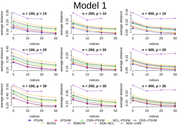
nslices a v er age distance n = 100, p = 10 5 10 20 50 0.10 0.20 0.30 nslices a v er age distance n = 100, p = 20 5 10 20 50 0.15 0.30 0.45 nslices a v er age distance n = 100, p = 30 5 10 20 50 0.25 0.40 0.55 nslices a v er age distance n = 200, p = 10 5 10 20 50 0.05 0.15 nslices a v er age distance n = 200, p = 20 5 10 20 50 0.10 0.25 nslices a v er age distance n = 200, p = 30 5 10 20 50 0.15 0.30 nslices a v er age distance n = 400, p = 10 5 10 20 50 0.04 0.10 0.16 nslices a v er age distance n = 400, p = 20 5 10 20 50 0.05 0.15 nslices a v er age distance n = 400, p = 30 5 10 20 50 0.10 0.20
Model 1
PSVM zPSVM CNN−PSVM NCL−PSVM OSS−PSVM BOSS fSMOTE ADA−NCL ADA−CNNFigure 1: Model 1 results. Some undersampling methods cannot run for smallnlarge
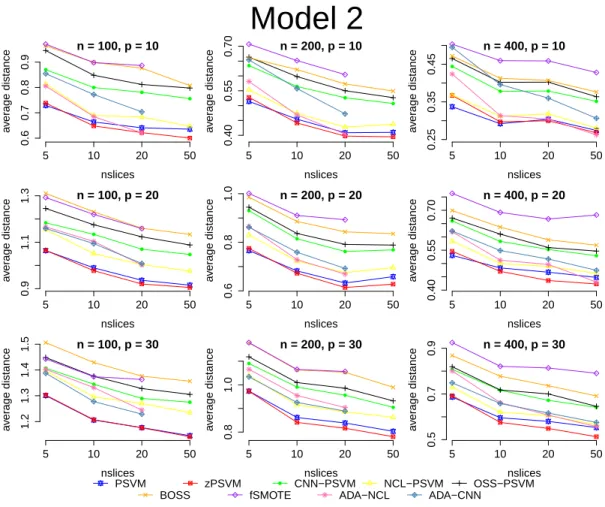
nslices a v er age distance n = 100, p = 10 5 10 20 50 0.6 0.7 0.8 0.9 nslices a v er age distance n = 100, p = 20 5 10 20 50 0.9 1.1 1.3 nslices a v er age distance n = 100, p = 30 5 10 20 50 1.2 1.3 1.4 1.5 nslices a v er age distance n = 200, p = 10 5 10 20 50 0.40 0.55 0.70 nslices a v er age distance n = 200, p = 20 5 10 20 50 0.6 0.8 1.0 nslices a v er age distance n = 200, p = 30 5 10 20 50 0.8 1.0 nslices a v er age distance n = 400, p = 10 5 10 20 50 0.25 0.35 0.45 nslices a v er age distance n = 400, p = 20 5 10 20 50 0.40 0.55 0.70 nslices a v er age distance n = 400, p = 30 5 10 20 50 0.5 0.7 0.9
Model 2
PSVM zPSVM CNN−PSVM NCL−PSVM OSS−PSVM BOSS fSMOTE ADA−NCL ADA−CNNFigure 2: Model 2 results. Some undersampling methods cannot run for smallnlarge
4
Simulation results
In this section we investigate the performance of these algorithms for the following 2 models:
Model I: Y =X1+X2+σε,
Model II: Y =X1/[0.5 + (X2+ 1)2] +σε,
where X ∼ Np(0,1) where p = 10,20,30, ε ∼ N(0,1), σ = 0.2, sample size n =
100,200,400 and the number of slices H= 5,10,20,50. To measure the performance of each algorithm we will be using the distance metric proposed by Li, Zha and Chiaromonte (2005):
dist(S1,S2) =kPS1−PS2k. (7)
where Si (i = 1,2) are two subspaces and PSi (i = 1,2) denotes the projection
matrices to the two subspaces. In our simulations, we will take the distance between the projection matrices of the true and estimated subspaces using the Frobenius norm. The smaller the distance, the better the algorithm.
Figures 1 and 2 show the results for the 2 models for the different algorithms. Since for each model we run 3 different sample sizes,n= 100,200,400 and 3 different dimensions p= 10,20,30 there are 9 graphs on each figure. In each graph, the y axis shows the distance between the true and estimated subspaces and the x axis shows the number of slices. As we can see most algorithms perform similarly, and for different models the algorithms seem to behave differently.
In Figure 1, we can see that for Model I all the methods except the two SMOTE algorithms perform similarly. The original PSVM algorithm performs overall the best but every other algorithm is relatively close. From the reweighting methods, zPSVM and ADA-NCL-PSVM perform better and overtake PSVM in performance as the number of predictors increases.
In Figure 2, we can see the results for Model II. In this model, zPSVM and ADA-NCL-PSVM perform better than every other algorithm including the classic PSVM. As the number of slices and the sample size increases, the combination of ADASYN and CNN (ADA-CNN-PSVM) also works very well. The two SMOTE algorithms, although much closer to the rest in this model, still perform worse on average.
These 2 models show clearly that reweighting can be helpful in most cases when using SVM algorithms for sufficient dimension reduction especially as the number of
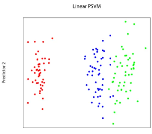
Figure 3: Applying linear PSVM to Iris data. It is clear that two of the three categories are not linearly separable
slices increases and therefore there is a much stronger imbalance between the two classes. It is also important to note that we don’t compare them to the two cost reweighting method by Artemiou and Shu (2014) because that method was based on a theoretical framework and therefore it is expected to outperform the methodology in this paper which are based on sample properties.
5
Data Analysis
In this section we will discuss the effectiveness of the reweight methodology in real datasets obtained from the UC Irvine machine learning repository (Bache and Lich-man (2013)). The first dataset is the well known Iris dataset and has categorical response. We check the classification performance of the algorithms even though SDR methodology is not necessarily a classification methodology because, as Li, Artemiou and Li (2011) explain in their discussion, it makes sense to view it as such when we have a categorical response. The other two datasets have continuous responses and regression is the main objective. Those are the computer hardware and the concrete slump test datasets.
5.1 Iris Dataset
The Iris dataset contains 150 flowers, and measures four variables (sepal length and width, petal length and width) in each one of these flowers. The flowers are divided
Table 1: Average percentage of separation between the three classes in the Iris Data
PSVM fSMOTE aSMOTE zPSVM CNN OSS BOSS SDC
17.88 21.50 24.92 17.41 7.45 6.75 7.17 17.28
into three species (Setosa, Vergicolour, Virginica) each with 50 flowers in the dataset. It is known that one category is well separated by the others, while the other 2 are closer together and some methods fail to distinguish completely between the two as shown in Figure 3
To compare the methods discussed in this work we run the following experiment 100 times. We randomly create 100 pairs of testing and training samples from the dataset. Each training sample contains 25 data points from each flower. We use the other 25 points for each flower as the testing set. We apply each of our methods to the training dataset to get the first direction of the data. For each method, we measure the percentage of samples where the testing points are separated for the three classes along the first direction. The average of the times we ran the experiment are given in Table 1. As we can see, the adaptive SMOTE has the highest percentage followed by the fixed SMOTE algorithm and then the SDC (Two cost SMOTE). We also note that zPSVM has similar performance to PSVM. The other imbalance correction methods do not perform very well.
5.2 Computer Hardware Dataset
The Computer Hardware dataset was first discussed in Ein-Dor and Feldmesser (1987). The objective is to create a regression model that estimates relative per-formance of the Central Processing Unit (CPU) of different computer models using some of its characteristics, including cache memory size, cycle time, minimum and maximum input/output channels and minimum and maximum main memory. There are 209 observations in the dataset.
Ein-Dor and Feldmesser (1987) found that the best model that fits the data gives large coefficient to the average main memory (as linear combination of the minimum and maximum) followed by the cache and then the cycle time. We ran the algorithms for dimension reduction using misclassification cost λ= 1 and the number of slices
H = 10. The CVBIC criterion of Li, Artemiou and Li (2011) for
deter-mining the dimension of CDRS suggests that d = 2. As Table 2 shows, the
methods differ slightly in the directions they recover. PSVM and z-PSVM give a very large coefficient to cycle time and the only other important coefficient is the one for
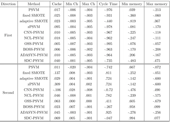
Table 2: Normalized coefficients for directions 1 and 2 on the Computer Hardware dataset for some of the methods discussed above.
Direction Method Cache Min Ch Max Ch Cycle Time Min memory Max memory
First PSVM .017 -.006 -.004 -.976 .039 -.213 fixed SMOTE .025 -.008 -.003 -.931 -.360 -.060 adaptive SMOTE .023 -.003 -.005 -.440 -.819 .367 zPSVM .095 -.004 -.005 -.978 -.081 -.170 CNN-PSVM .010 -.005 -.003 -.967 -.225 -.118 NCL-PSVM .018 -.005 -.004 -.962 -.247 -.111 OSS-PSVM .005 -.007 -.003 -.995 -.076 -.057 BOSS-PSVM .006 -.006 -.002 -.963 -.170 -.208 ADASYN-PSVM .010 -.005 -.003 -.964 .206 -.167 SDC-PSVM .040 -.001 -.005 -.735 -.483 .475 Second PSVM .011 -.020 -.004 -.742 .667 -.072 fixed SMOTE .137 .008 -.003 .811 -.252 -.051 adaptive SMOTE .029 .004 -.001 .724 -.142 -.600 zPSVM .309 .004 .002 .724 -.142 -.600 CNN-PSVM -.106 .028 -.008 -.0.72 -.476 .490 NCL-PSVM .046 -.008 .001 .782 -.239 -.575 OSS-PSVM .063 .000 .000 .411 .605 -.679 BOSS-PSVM .023 .007 -.001 -.267 .958 .099 ADASYN-PSVM .045 -.003 -.001 .925 -.276 -.256 SDC-PSVM .069 .005 -.001 -.047 .994 .077
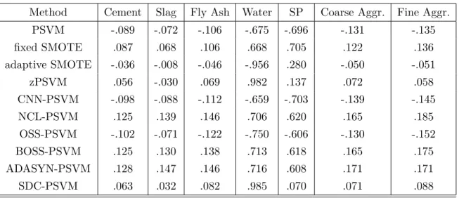
Table 3: Normalised coefficients for the main direction on the Concrete Slump Test dataset for some of the methods discussed above
Method Cement Slag Fly Ash Water SP Coarse Aggr. Fine Aggr.
PSVM -.089 -.072 -.106 -.675 -.696 -.131 -.135 fixed SMOTE .087 .068 .106 .668 .705 .122 .136 adaptive SMOTE -.036 -.008 -.046 -.956 .280 -.050 -.051 zPSVM .056 -.030 .069 .982 .137 .072 .058 CNN-PSVM -.098 -.088 -.112 -.659 -.703 -.139 -.145 NCL-PSVM .125 .139 .146 .706 .620 .165 .185 OSS-PSVM -.102 -.071 -.122 -.750 -.606 -.130 -.152 BOSS-PSVM .125 .130 .138 .713 .618 .165 .175 ADASYN-PSVM .128 .147 .146 .716 .608 .171 .171 SDC-PSVM .063 .032 .082 .985 .070 .071 .088
maximum main memory. Fixed SMOTE is similar but the second largest coefficient is assigned to the minimum main memory. CNN, NCL, OSS, BOSS and ADASYN give a very large coefficient to cycle time and then approximately similar coefficients to the maximum and minimum main memory variables. Two cost SMOTE give a slightly smaller coefficient on cycle time and significant coefficients to both maximum and minimum memory. Finally, adaptive SMOTE give the maximum coefficient to the minimum main memory and a significant coefficients to cycle time and maximum memory.
It is worth noting that, although the authors showed that cache memory size is the second most important variable in the model, none of the methods give a relatively large coefficient in the first direction (the largest is given by zPSVM which is 0.095 and it is the only method that puts it as the third most important variable in the first dimension). On the second direction, zPSVM is the only method that give a large coefficient to cache memory size with value 0.309 which shows that it is the only method that it captures something other methods are not able to do.
5.3 Concrete slump test
The third dataset we discuss in this work is the concrete slump dataset obtained from the UC Irvine Data repository which was first studied in Yeh (2007). There are 7 predictors: cement, slag, fly ash, water, superplasticizer (SP), coarse aggregate,
and fine aggregate; the response variable is the concrete flow. It is known that the concrete flow is mainly affected by the water content in the concrete mixture and there is less effect from the other variables. We run the 10 methods listed in Table 3 using misclassification cost λ= 1 and number of slices H = 10.
As we can see from the results of Table 3, all the methods indicate the effect water has on the concrete flow on the first direction. Most of the methods split the effect on the main direction between water and superplasticizer (SP) and only two cost SMOTE (SDC), zPSVM and adaptive SMOTE suggest water being the most significant variable in the main direction.
6
Discussion
Sufficient Dimension Reduction (SDR) is a set of dimension reduction tools that can be used in a regression setting to find a few linear or nonlinear functions of the predictors that describe the regression surface. Lately, SDR has increased in popularity and there is a huge selection of algorithms to choose from, each one with its own advantages and disadvantages. PSVM is one of the new algorithms (see Li, Artemiou and Li (2011)) with the main advantage being the fact that it uses SVM which allow it to achieve linear and nonlinear dimension reduction under a unified framework. The algorithm of PSVM is constructed in such a way that there is imbalance between the size of the two classes in most comparisons.
In this work, we have run a simulation study of several reweighting algorithms to reduce the effect that imbalance classes have on dimension reduction. The algorithms we used are well known in the classification framework and under specific circum-stances work much better than the classic SVM algorithm in improving the accuracy of the prediction. As we can see in the simulation results, this is not so much the case in the dimension reduction framework. We can see that while some algorithms like zPSVM give improved results most of the times in the dimension reduction frame-work, some others failed, i.e. SMOTE which is considered an excellent method for treating imbalance in classification.
There are many possible reasons why this might be the case. First, in the di-mension reduction framework we are not interested in misclassifications but rather in hyperplane alignment between the different classifications of the data. Second, these methods are based on sample observations and not on any established theoretical properties.
perform better than all other algorithms we discuss here. It is among the best two methods in almost every parameter combination in the simulation section and it is the method that recovers something meaningful in all 3 real datasets we use in this paper.
This study can be extended in several directions. One possible direction is how these ideas extend to the nonlinear dimension reduction. Although these algorithms in the classification framework work similarly for linear and nonlinear kernels, there is a difference in the dimension reduction framework. In the dimension reduction framework, we use multiple comparisons and combine them into a single candidate matrix; this process gets complicated in the nonlinear case. This needs to ensure that the same number of Support Vectors are used each time which may not be the case. Therefore we need to see this in more depth in a separate work.
Another interesting aspect might be the development of new reweighting algo-rithms designed with the dimension reduction problem in mind. As it was mentioned in the introduction, the problem in dimension reduction is not minimizing the number of misclassifications but the alignment of the hyperplane with the regression surface. Therefore, one can construct algorithms that optimise the estimation of ψ by con-sidering the angles between the hyperplanes. One example is to modify zPSVM and instead of estimating z using the geometric mean, estimating it using the average angle between the estimated hyperplanes.
Acknowledgement
The authors would like to thank an Editor and an anonymous reviewer for their valuable contributions which improved the contents of the manuscript. The authors would like to thank the London Mathematical Society who funded Luke Smallman through an Undergraduate Research Bursary award (URB14-17) for this work. References
1. Artemiou, A. and Shu, M. (2014). A cost based reweighed scheme of Prin-cipal Support Vector Machine. Topics in Nonparametric Statistics, Springer Proceedings in Mathematics and Statistics, 74, 1–22
2. Bache, K. and Lichman, M. (2013). UCI Machine Learning Repository [http://archive.ics.uci.edu/ml]. Irvine, CA: University of California, School of Information and Computer
3. Batista, G. E. A. P. A., Prati, R. C. and Monard M. C. (2004). A study of the behavior of several methods for balancing Machine Learning training data. ACM SIGKDD Explorations Newsletter,6, 20–29.
4. Chawla, N. V., Bowyer, K. W., Hall, L. O. and Kegelmeyer, W. P. (2002) SMOTE; Synthetic Minority Over-sampling Technique, Journal of Artificial Intelligence,16, 321–357.
5. Cook, R. D. (1998). Principal Hessian directions revisited (with discussion) Journal of the American Statistical Association,93, 84–100.
6. Cook, R. D. and Weisberg, S. (1991). Discussion of “Sliced inverse regression for dimension reduction”. Journal of the American Statistical Association. 86,
316–342.
7. Ein-Dor, P., Feldmesser, J. (1987). Attributes of the performance of central processing units: A relative performance prediction model Communications of the ACM,30, 4, 308–317.
8. Fukumizu, Bach, and Jordan (2009). Kernel dimension reduction in regression. The Annals of Statistics,37, 1871 – 1905.
9. Hart, P. E. (1968). The condensed nearest neighbor rule. Transaction on In-formation Theory IT-14, 515–516.
10. He, H., Bai, Y., Garcia, E. A. and Li, S. (2008). ADASYN: Adaptive Synthetic Sampling Approach for Imbalanced Learning. In Proceedings of the Interna-tional Joint Conference of Neural Network, 1322–1328.
11. He, H. and Garcia, E. A. (2009). Learning from Imbalanced Data. IEEE Transactions on Knowledge and Data Engineering,21, 9, 1263–1284.
12. Imam, T., Ting K. M. and Kamruzzaman, J. (2006) z-SVM: an SVM for Im-proved Classification of Imbalanced Datasets. AI 2006: Advances in Artificial Intelligence, 264–273.
13. Kubat, M. and Matwin, S. (1997). Addressing the course of Imbalanced Train-ing Sets: One Sided SamplTrain-ing. InInternational Conference of Machine Learn-ing, 179–186.
14. Laurikkala, J. (2001). Imporving identification of difficult small classes by bal-ancing class distribution. Tecnical Report, A-2001-2 University of Tampere.
15. Lee, K. K., Gunn, S. R., Harris, C. J. and Reed, P. A. S. (2001). Classification of imbalanced data with transparent kernels. InProceedings of International Joint Conference on Neural Networks (IJCNN ’01), 4, 2410 – 2415, Washington, D.
C.
16. Li, B., Artemiou, A. and Li L. (2011). Principal Support Vector Machine for linear and nonlinear sufficient dimension reduction. The Annals of Statistics,
39, 3182–3210
17. Li, B. and Wang, S. (2007). On directional regression for dimension reduction. Journal of the American Statistical Association,102, 997–1008.
18. Li, B., Zha, H., and Chiaromonte, F. (2005). Contour regression: a general approach to dimension reduction. The Annals of Statistics,33, 1580-1616.
19. Li, K. -C. (1991). Sliced inverse regression for dimension reduction (with dis-cussion). Journal of the American Statistical Association,86, 316 – 342.
20. Li, K. -C. (1992). On principal Hessian directions for data visualization and dimension reduction: another application of Stein’s lemma. Journal of the American Statistical Association,86, 316 – 342.
21. Tomek, I. (1976). Two modifications of CNN. IEEE Transactions in System, Man, Cybernetics,6, 769–772
22. Wu, H. M. (2008). Kernel sliced inverse regression with applications on classi-fication. Journal of Computational and Graphical Statistics,17, 590–610.
23. Yeh, I.-C. (2007). Modeling slump flow of concrete using second-order regres-sions and artificial neural networks. Cement and Concrete Composites, 29, 6, 474–480.
24. Yeh, Y.-R., Huang, S.-Y., and Lee, Y.-Y. (2009). Nonlinear Dimension Reduc-tion with Kernel Sliced Inverse Regression. IEEE Transactions on Knowledge and Data Engineering,21, 1590–1603.
25. Yin, X., Li, B., and Cook, R.D. (2008). Successive direction extraction for estimating the central subspace in a multiple-index regression. Journal of Mul-tivariate Analysis. 99, 1733 – 1757.