A Selective Sampling Method for Imbalanced Data Learning on Support Vector Machines

2010

A Selective Sampling Method for Imbalanced Data

Learning on Support Vector Machines

Jong Myong Choi

Iowa State University

Follow this and additional works at:https://lib.dr.iastate.edu/etd Part of theIndustrial Engineering Commons

This Dissertation is brought to you for free and open access by the Iowa State University Capstones, Theses and Dissertations at Iowa State University Digital Repository. It has been accepted for inclusion in Graduate Theses and Dissertations by an authorized administrator of Iowa State University Digital Repository. For more information, please [email protected].

Recommended Citation

Choi, Jong Myong, "A Selective Sampling Method for Imbalanced Data Learning on Support Vector Machines" (2010).Graduate Theses and Dissertations. 11529.

by

Jong Myong Choi

A dissertation submitted to the graduate faculty

in partial fulfillment of the requirements for the degree of

DOCTOR OF PHILOSOPHY

Major: Industrial Engineering

Program of Study Committee: John K. Jackman, Major Professor

Sigurdur Olafsson Douglas D. Gemmill

Dianne H. Cook Anthony M. Townsend

Iowa State University

Ames, Iowa

2010

TABLE OF CONTENTS LIST OF TABLES ... iv LIST OF FIGURES ... v ACKNOWLEDGEMENTS ... vi ABSTRACT…. ... vii CHAPTER 1 INTRODUCTION ... 1

CHAPTER 2 LITERATURE REVIEW ... 4

2.1 Handling the Class Imbalance Problem ... 4

2.1.1 Changing class distributions ... 5

2.1.2 Adjusting classifiers to imbalanced data sets ... 9

2.1.2 Ensemble learning methods ... 12

2.2 Performance Measures for Imbalanced Data Learning ... 14

2.3 Summary and Research Scope ... 17

CHAPTER 3 CLASS IMBALANCE PROBLEM WITH SUPPORT VECTOR MACHINE LEARNING ... 19

3.1 Support Vector Machine (SVM) Classifier ... 19

3.2 SVMs and the Skewed Boundary ... 26

3.3 Problems associated with SVM classifier for imbalanced data ... 28

3.4 Effectiveness of rebalancing class distribution ... 29

3.5 Hypotheses ... 34

CHAPTER 4 SELECTIVE SAMPLING USING A GENETIC ALGORITHM ... 35

4.1 SVMs for Large-Scale Datasets ... 35

4.2 Genetic Algorithm for Under-sampling of the Majority Class ... 36

4.3 Experiments ... 41

4.3.1 Experimental Design ... 41

4.3.2 Approaches for imbalanced data learning ... 43

4.4 Experimental Results and Discussion ... 47

CHAPTER 5 SMALLER LEARNING SETS for IMBALANCED DATA LEARNING with SVMs ... 49

5.1 A new method to reduce learning time ... 49

5.1.1 Stage1. Rough elimination of support vectors of the majority class in kernel space ... 51

5.1.2 Stage2. Selection of majority instance support vectors ... 53

5.2 Demonstration of GA-SS ... 59

5.2.2 Gaussian radial-based kernel function case ... 62

5.3 Experiments with real datasets... 64

5.4 Summary and Discussions ... 68

CHAPTER 6 CONCLUSIONS ... 73

APPENDIX A. EXPERIMENTAL IMBALANCED TRAINING SETS ... 77

APPENDIX B. PARAMETER C AND



APPENDIX C. INITIAL CLASSIFICATION RESULTS on SVM LEARNING WITH THE ORIGINAL TRAINING AND TEST DATASETS ... 84

APPENDIX C. INITIAL CLASSIFICATION RESULTS on SVM LEARNING WITH THE ORIGINAL TRAINING AND TEST DATASETS ... 85

APPENDIX D. MEAN DIFFERENCE BEWTEEN g-mean OF the training set IN TERMS OF THREE APPROACHES (SVM-SMOTE, SVM-RU and GA-IS) ... 86

APPENDIX E. MEAN DIFFERENCE BEWTEEN g-mean OF the training set CORRESPONDING TO ITERATIONS CHOSEN FOR INSTANCE SELECTION ... 89

APPENDIX F. SELECTED INSTANCES FOR LEARNING FROM GENETIC ALGORITHM BASED INSTACE SELECTION APPROACH ... 90

LIST OF TABLES

Table 2.1 Cost matrix ... 10

Table 2.2 Confusion matrix for performance evaluation ... 15

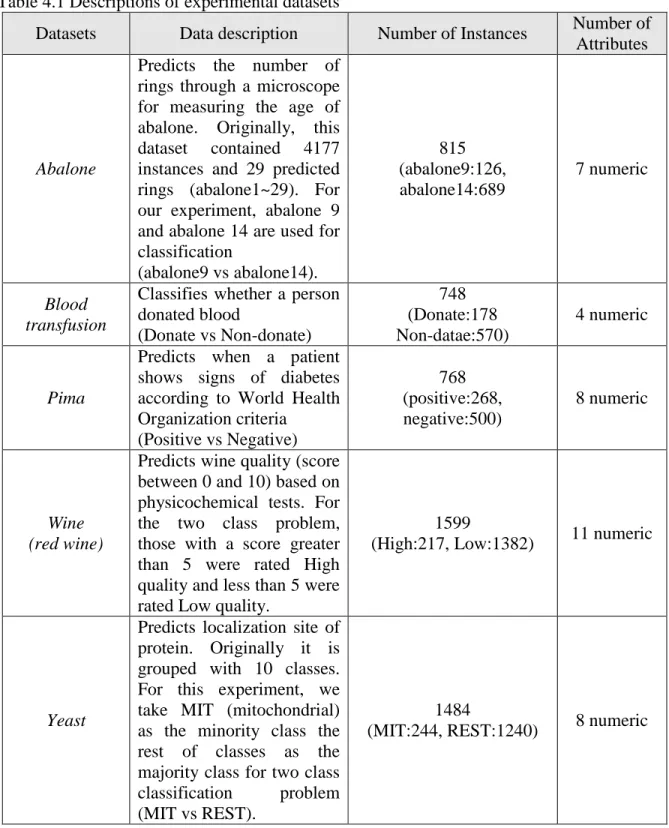
Table 4.1 Descriptions of experimental datasets ... 42

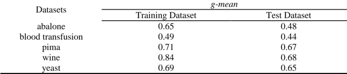
Table 4.2 G-mean values of the experimental datasets on SVM (training and test sets) ... 43

Table 4.3 Average G-mean of Training sets obtained from 4 different methods ... 47

Table 5.1 Improvement of G-mean and training set reduction after Stage2 ... 68

LIST OF FIGURES

Figure 2.1 Synthetic over-sampling example by SMOTE algorithm ... 7

Figure 3.1 Linear separating hyperplanes for the separable case ... 20

Figure 3.2 Linear separating hyperplanes for the non-separable case ... 24

Figure 3.3 Example of class imbalance problem on SVMs ... 29

Figure 3.4 Boundary movements by SMOTE algorithm ... 31

Figure 3.5 Boundary movements by random under-sampling ... 33

Figure 4.1 GA-based Instance Selection from the majority instances ... 40

Figure 4.2 Class distributions of experimental datasets (abalone and yeast) ... 43

Figure 4.3 Average g-mean values of the training dataset in terms of increase of synthetic minority instances by SMOTE... 45

Figure 5.1 Stage 1 Algorithm... 53

Figure 5.2 Boundary sensitivity to removing one SV instance ... 54

Figure 5.3 GA-SS Algorithm ... 57

Figure 5.4 Boundary movement through selecting instances in Stage2 ... 57

Figure 5.5 Overall procedure of our approach for imbalanced training datasets ... 58

Figure 5.6 Decision boundaries at each iteration through selecting instances from SVs of the majority class (linear kernel function) ... 60

Figure 5.7 Mapping decision boundaries at Iteration 1 and 2 on the original training set ... 60

Figure 5.8 A decision boundary that produces the maximum G-mean for the original training set ... 61

Figure 5.9 Decision boundaries for Stage 1 iterations ... 63

Figure 5.10 Mapping decision boundaries for Iterations 2 and 3 on the original training dataset ... 63

Figure 5.11 Decision boundary that produces the maximum G-mean of the original training set through GA-SS ... 64

Figure 5.12 Trend of G-mean values of the original training set on reduction of the majority instances in Stage1 ... 65

Figure 5.13 Box plots of G-mean of the training set after Stage 2 for ... 67

Figure 5.14 Comparison of G-mean values for the training sets (average) for 5 different methods ... 70

Figure 5.15 Size of training sets ... 71

ACKNOWLEDGEMENTS

It is a pleasure to thank many people who helped me conduct research toward a Ph.D. and

write this dissertation. This work would not have been finished without their support and

patience.

First, I would like to heartily express the deepest appreciation to my adviser, Dr. John

Jackman for his encouraging way to help me whenever I am in a trouble during my graduate

school years. His persistent guidance enabled me to complete this work. I am also thankful to my

committee members, Dr. Sigurdur Olafsson, Dr. Doug Gemmill, Dr. Anthony Townsend and Dr.

Dianne Cook whose valuable and helpful comments improved this work.

I also would like to thank my family members: my parents for educating me with

unconditional support to finish my study. Especially, my special thanks goes to my wife, In Suk

Lee who always understands and encourages me with her support, patience and endless love

ABSTRACT

The class imbalance problem in classification has been recognized as a significant research

problem in recent years and a number of methods have been introduced to improve classification

results. Rebalancing class distributions (such as over-sampling or under-sampling of learning

datasets) has been popular due to its ease of implementation and relatively good performance.

For the Support Vector Machine (SVM) classification algorithm, research efforts have focused

on reducing the size of learning sets because of the algorithm‟s sensitivity to the size of the

dataset. In this dissertation, we propose a metaheuristic approach (Genetic Algorithm) for

under-sampling of an imbalanced dataset in the context of a SVM classifier. The goal of this approach

is to find an optimal learning set from imbalanced datasets without empirical studies that are

normally required to find an optimal class distribution. Experimental results using real datasets

indicate that this metaheuristic under-sampling performed well in rebalancing class distributions.

Furthermore, an iterative sampling methodology was used to produce smaller learning sets by

removing redundant instances. It incorporates informative and the representative under-sampling

mechanisms to speed up the learning procedure for imbalanced data learning with a SVM. When

compared with existing rebalancing methods and the metaheuristic approach to under-sampling,

this iterative methodology not only provides good performance but also enables a SVM classifier

to learn using very small learning sets for imbalanced data learning. For large-scale imbalanced

datasets, this methodology provides an efficient and effective solution for imbalanced data

CHAPTER 1 INTRODUCTION

The imbalanced learning problem in data mining has attracted a significant amount of

interest from the research community and practitioners because real-world datasets are

frequently imbalanced, having a minority class with relatively few instances when compared to

the other classes in the dataset. Standard classification algorithms used in supervised learning

have difficulties in correctly classifying the minority class. Most of these algorithms assume a

balanced distribution of classes and equal misclassification costs for each class. In addition,

these algorithms are designed to generalize from sample data and output the simplest hypothesis

that best fits the data. This principle is embedded in the inductive bias of many machine learning

algorithms including Decision Tree, nearest neighbor, and Support Vector Machine (SVM).

Therefore, when they are used on complex imbalanced data sets, these algorithms are inclined to

be overwhelmed by the majority class and ignore the minority class causing errors in

classification for the minority class. In other words, standard classification algorithms try to

minimize the overall classification error rate by producing a biased hypothesis which regards

almost all instances as the majority class.

Recent research on the class imbalance problem has included studies on datasets from a

wide variety of contexts such as, information retrieval and filtering (Lewis & Catlett, 1994),

diagnosis of rare thyroid disease (Murphy & Aha, 1994), text classification (Chawla et al., 2002),

credit card fraud detection (Wu & Chang, 2003) and detection of oil spills from satellite images

(Kubat et al., 1998). The degree of imbalance varies depending on the context. In intrusion

detection, typically less than 10% of the data are actual intrusions. In detection of cancerous

To illustrate the imbalance problem, consider the “Mammography Data Set”, which has

been used frequently to study the class imbalance learning problem. This data is a collection of

images obtained from a series of mammography exams conducted on a set of distinct patients.

Analyzing the images in the two classes, “cancerous” and “noncancerous” patient, it is observed

that the number of noncancerous patients greatly exceeds the number of cancerous patients.

Indeed, this data set contains 10,923 “Negative” (major class) samples and 260 “positive”

(minority class) samples. Ideally, a classifier should classify both classes with almost 100%

accuracy. However, classifiers tend to produce severely biased classification with the majority

class almost 100% accuracy and conversely the minority class having accuracies of less than

0.5% accuracy. As a result, most cancerous patients are classified as noncancerous (i.e., a Type I

error). In the classification of diagnosing patients, such a consequence would be extremely costly

because treatment would not be initiated. For these imbalanced scenarios, classifiers should

provide much higher accuracy for the minority class without a significant loss in accuracy for the

majority class.

New classification methods are needed to address the class imbalance problem in

supervised learning. In this research, we propose a new methodology for imbalanced data

learning based on the SVM classification algorithm. The remainder of the dissertation is

organized as follows. In Chapter 2, we review general approaches for imbalanced data learning

and related studies and describe the scope of this research. Chapter 3 briefly describes the SVM

classification algorithm and the causes of imbalanced learning with the SVM classifier. This is

followed by a discussion of existing methods that have been used for the class imbalance

problem based on the SVM algorithm. At the end of this chapter, the approach used in the new

„large-scale data’, and an optimization based under-sampling method using Genetic Algorithm is introduced and classification results are compared with other sampling methods using real

datasets. In Chapter 5, the new methodology that solves the class imbalance problem on SVM

with relatively small learning sets for SVM classifier is described. Finally we conclude with

CHAPTER 2 LITERATURE REVIEW

In general, a class imbalance problem is seen in two situations namely, natural imbalance

or rarity of cases (i.e., instances or samples). Underlying reasons for imbalance could be the lack

of occurrences in nature for a specific phenomena or possibly insufficient funds or time to collect

sufficient data. In recent years, many researchers have studied the class imbalance problem.

Weiss (2004) presented an overview of the field of learning from imbalanced datasets. His work

particularly focused on the problems with identifying rare objects in data mining by defining two

types of rarity: rare classes and rare cases. A rare class contains relatively smaller instances than

other classes, while a rare case indicates a small subset of the data (instance) space.

Unsupervised learning algorithms such as clustering may help to identify a rare case. More

generally, class imbalance is related to rare classes and is associated with classification

problems. In his work, Weiss argued that typical evaluation metrics do not adequately describe

the value of rarity so that data mining is not likely to handle rare classes and rare cases. Monard

et al. (2002) discussed several issues related to learning with skewed class distributions, such as

the relationship between cost-sensitive learning and class distributions, and the limitations of

accuracy and error rate in measuring the performance of classifiers.

2.1 Handling the Class Imbalance Problem

The various approaches used to deal with the class imbalance problem can be grouped

into three categories: (1) changing class distributions (modifying the data itself to rebalance

algorithms to imbalanced data sets by applying cost or weight for misclassified cases), and (3)

ensemble learning methods (using a combination of multiple classifiers with multiple datasets).

2.1.1 Changing class distributions

Changing class distributions is performed at the data level in order to modify class

distribution in the training datasets. Since many more instances belong to the majority class than

the minority class, class distribution can be balanced by under-sampling the majority class,

over-sampling the minority class, combining under-over-sampling and over-over-sampling, or some other

sampling method. Studies have shown that a balanced data set provides improved classification

performance as compared with an imbalanced data set. There have been numerous studies on

changing class distribution (Laurikkala, 2001 and Estabrooks et al., 2004). Also, Weiss (2003)

investigated the effect of class distribution on decision tree classification by changing class

distributions to achieve different ratios and measuring performance using accuracy and Area

Under the Curve (AUC). Three basic techniques are used in balancing classes namely, heuristic

and non-heuristic under-sampling, heuristic and non-heuristic over-sampling, and advanced

sampling. Japkowicz (2000) compared multiple balancing methods and concluded that both

under-sampling and over-sampling are very effective methods for dealing with the class

imbalance problem.

Over-sampling

One simple over-sampling method is random over-sampling. Its mechanism is adding a

set E of additional instances (i.e., instance duplicates) randomly sampled from the minority class

by E and as a result, the class distribution is more balanced. This provides a mechanism for

varying the degree of class distribution balance to any desired balance level. Over-sampling does

not increase information; instead by replication it raises the weight of the minority samples. The

problem with over-sampling is that an over-fitting problem will generally occur, which causes

the classification rule to become too specific; even though the accuracy for training set is high,

the classification performance for new test datasets will likely be worse. By appending

duplicated data to the original data set, some of the data copied becomes too specific and

classifiers will produce multiple clauses for the duplicate data (Kubat and Martin, 1997).

To avoid the over-fitting problem in over-sampling, Chawla et al. (2002) suggested a

heuristic over-sampling method, called Synthetic Minority Over-sampling Technique (SMOTE),

which has worked well in various applications. SMOTE is considered to be one of the

state-of-the-art approaches for imbalanced learning. This method generates synthetic data based on the

feature space similarities between existing minority instances considering the K-nearest

neighbors for each minority instance. In order to create a synthetic instance, it finds the K-nearest

neighbors of each minority instance, randomly selects one of them, and then multiplies the

corresponding feature vector difference with a random number between 0 and 1 to produce a

new minority instance in the neighborhood. Figure 1 shows an example of the SMOTE

procedure. This synthetic over-sampling avoids the over-fitting problem and also causes the

decision boundaries for the minority class to move towards the majority class. As a variant of

SMOTE, Han et al. (2005) introduced Borderline_SMOTE which only oversamples synthetic

instances of the minority class near the decision boundary since those instances are most likely to

be misclassified. Results were better when compared to standard SMOTE and random

method, Adaptive Synthetic Sampling (ADASYN), that uses a density distribution of the

minority instance as a criterion to automatically decide the number of synthetic samples

generated for each minority instance. ADASYN generates a new instance by calculating the class

ratio of the minority and majority instances in the K-nearest neighbors of each minority instance.

As a result, more synthetic instances are generated for minority class instances that are harder to

learn compared to instances that are easier to learn. This approach improved learning with

respect to the data distributions on the imbalanced data sets by reducing the bias of class

distribution and by adaptively shifting the decision boundary to put more attention on instances

difficult to learn.

( )

is a random number between 0 and 1

syn i knn i

x x x x 



   

Figure 2.1 Synthetic over-sampling example by SMOTE algorithm

Under-sampling

While over-sampling adds instances to the original data set, under-sampling removes

instances from the majority class while keeping all instances of the minority class due to rareness Generated synthetic instance x_syn

of information. A simple method for sampling the majority class is random

under-sampling, a non-heuristic method that balances class distributions by selecting and removing

majority instances randomly. Several heuristic under-sampling methods have been proposed

from data cleaning in recent years. They are based on either of two different noise model

hypotheses: one is that instances near to a decision boundary between two classes are considered

noise, while the other considers that instances having more neighbors from different classes are

noise.

Since random under-sampling leads to losing potentially useful data, some heuristic

under-sampling methods try to remove superfluous instances which will not affect the

classification accuracy of the training set. Hart (1968) introduced a training set condensation

algorithm, Condensed Nearest Neighbor Rule (CNN), in order to find a consistent subset of a

sample set which can correctly classify all of the remaining instances in the training set. The

algorithm uses two bins, called S and T. Initially, the first sample of the training set is placed in

S, while the remaining samples of the training set are placed in T. Then one pass through T is

performed. During the scan, whenever a point in T is misclassified by using S as the training set,

it is transferred from T to S. After classification, process is repeated until no points are

transferred from T to S. The motivation for this heuristic is that misclassified data lies close to

the decision boundary. In the same manner, Tomek (1976) proposed an effective method to

eliminate data in the overlapping regions. Given two instances x and y that have a different class

label and are separated by a distance d(x,y), the pair (x, y) is called a Tomek link if there is no instance z such that d(x,z)d(x,y)or d(y,z)d(x,y). Instances participating in Tomek links

are considered either borderline or noisy. Kubat and Matin (1999) proposed one-sided sampling

minority instances since they are rare, (even though some of them can be noisy) and instead

prune out only majority instances. Initially it starts with a subset(C) of training set (S) that

contains all minority instances, C S, and using a 1-Nearest Neighbor rule using instances in

C, classify the instances in S. Afterwards, all misclassified instances are moved to C, then all

majority instances participating in Tomek links from C are removed since theyare believed to be

borderline and/or noisy. Wilson (1972) introduced the Edited Nearest Neighbor Rule (ENN) to

remove any instance whose class label is different from the class of at least two of its three

nearest neighbors. The idea behind this technique is to remove the instances from the majority

class that are near or around the borderline of different classes based on the concept of nearest

neighbor (NN) in order to increase classification accuracy of minority instances rather than

majority instances.

2.1.2Adjusting classifiers to imbalanced data sets

Rebalancing the data distribution through either over-sampling or under-sampling has

had some success, but the methods are usually computationally expensive. Also, changing class

distribution at the data level does not always lead to better classification performance. A

classifier is not always influenced by class distributions. Drummond and Holte (2003) observed

that over-sampling did not produce effective improvement in performance or there was no

change in classification. On the contrary, over-sampling prunes less than under-sampling using

the default parameters for the C4.5 algorithm. A modification of the parameter settings of C4.5

improved classification performance and avoided the over-fitting problem during over-sampling.

Thus, while sampling methods have tried to balance class distribution by considering the

introduced for imbalanced data learning. One is the cost sensitive method, which uses a cost

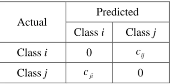
matrix to penalize misclassification of instances, as shown in Table 2.1. Typically, no costs are

applied to the correctly classified cases and the cost of misclassifying minority cases is higher

than that of majority cases. The objective of this strategy is to minimize the cost of

misclassification. In some applications, cost sensitive techniques have performed better than

sampling methods (McCarthy et al., 2005 and Liu et al., 2006).

Actual Predicted Class i Class j

Class i 0 cij

Class j cji 0

Table 2.1 Cost matrix

MetaCost (Domingos, 1999) is another method related to cost-sensitive learning. It

estimates class probabilities using Bagging and then re-labels the training instances with their

minimum expected classes, and in the end, relearns a model using the modified training set.

Based on the weight update rule of AdaBoost (Freund & Schapire, 1997) for misclassified

instances at an iterative learning, Fan et al. (1999) proposed a discriminant weight update method

for misclassified instances for imbalanced datasets, which is called Adacost. Their approach is to

assign larger weights for misclassified instances belonging to the minority class than those

belonging to the majority class and as a result, Adacost has performed empirically better in

Some classifiers such as the Naïve Bayes classifier or some Neural Networks use a score

to show the degree to which an instance belongs to a class. This type of ranking can be used in

alternative classifiers by changing the threshold for an instance belonging to a class (Weiss,

2004). For biasing the discrimination procedure, Barandela et al. (2003) proposed a weighted

distance function in classification instead of altering the class distributions in terms of a nearest

neighbor (NN) classifier. Supposing that d_e( ) is the Euclidean metric, xnew a new instance to

classify, x₀ a training sample from class i, n_i the number of instances of class i and m the

dimensionality of the input variable, a weighted distance function, d_w( ) is defined as:

1/

0 0

( , ) ( / ) m ( , )

w new i e new

d x x  n n d x x . This could assign greater weighting factors to majority instances than minority instances; consequently, producing smaller distances to instances of the

minority class than distances to those of the majority class. As a result, the neighbors of the new

instances are found among the minority instances, increasing the value of the geometric mean

(g-mean). For the SVM classification algorithm, this biasing approach pushes a hyperplane further

away from the minority (positive) class for imbalanced datasets. Wu and Chang (2003) proposed

a biasing algorithm to change the kernel function. Biasing classification algorithms in SVM

using larger penalty constants associated with the minority class made misclassification errors

for the minority instances much costlier than errors for majority instances (Veropoulos et al.,

1999). Huang at el. (2004) proposed a Biased Minimax Probability Machine (BMPM) to resolve

learning for imbalanced datasets. Given the mean and covariance matrices of the majority and

minority classes, BMPM formulates an optimization problem to find the decision hyperplane by

adjusting the lower bound of the accuracy for the classification of the future data. For example, if

optimization tries to maximize it by setting the lower bound of the classification accuracy for

both classes. Achieving the worst case accuracy for the minority can be avoided while

maintaining the acceptable accuracy level of the majority class in imbalanced data learning.

One-class learning is an alternative to discrimination where the model is created based on

the instances of the target class alone. The main idea is that boundaries between two classes are

estimated from data of one class (the target class) so that this approach is not sensitive to the

class distribution in the training set. A boundary around the target class is defined in such a way

that most of the target objects are included and at the same time the chance of accepting outlier

objects is minimized. For instance, Kubat et al. (1998) introduced the SHRINK algorithm

following this general principle and applied it to detecting rare oil spills from satellite radar

images. The goal was to find the classification rule that best identifies the positive examples (oil

spills) using a g-mean measure. Assuming that the negative (majority) instances outnumber

positive (minority) instances, the algorithm labeled the mixed regions as positive (minority). This

alters the learner‟s focus: search for the best positive region, one with the maximum ratio of positives to negatives. Raskutti and Kowalczyk (2004) studied one-class learning with highly

imbalanced dataset learning using a SVM classifier. They showed that one-class learning is

useful for extremely imbalanced datasets with a high dimensional noisy feature space.

2.1.2 Ensemble learning methods

Ensemble learning is motivated by the information loss that occurs in under-sampling. In

ensemble learning, multiple classifiers are generated by training subsets from the original

dataset. In the end, the classifiers are combined in a learning process and the final classification

successful approaches. Most boosting algorithms use iteratively learning weak classifiers that

have been produced by placing different weights on the training instances. In each iteration,

boosting increases weights for incorrectly classified instances and decreases weights for

correctly classified ones, placing more attention on the incorrectly classified instances for the

next iteration. Rare-Boost scales false-positive instances in proportion to how well they are

differentiated from true-positive instances and scales false-positive instances in proportion to

how well they are distinguished from true-negative instances (Joshi et al., 2001). SMOTEBoost

(Chawla et al., 2003) addressed the issue that boosting may produce an over-fitting problem as in

over-sampling. Instead of updating weights to change distributions of the training dataset, it adds

new instances of the minority class using SMOTE. Chan and Stolfo (2001) proposed another

ensemble method conceptually similar to a Bagging approach. They conducted some preliminary

experiments to identify a desired class distribution that avoids the class imbalance problem, and

then resampled to make multiple training sets based on the desired class distribution. Each

training set contained all instances of the minority class and a subset of the majority instances.

To use all instances of the majority class, each majority class instance appeared in at least one

training set. Finally, the learning algorithm was applied to each training set and a composite

learner was created from the classification results of all classifiers.

Recently, two algorithms, EasyEnsemble and BalanceCascade have been introduced (Liu

et al., 2006). The strategy of these two methods is to make several training sets by keeping all the

minority instances and under-sampling several subsets from the majority class. With replacement

in sampling of the majority class, they overcome potential of information loss of the majority

class. EasyEnsemble independently samples (with replacement) from the majority class several

classifiers for the subsets. In other words, EasyEnsemble generates T balanced training sets. The

output of learning the ith training set is an AdaBoost classifier Hi (i = 1,..,T). Then all generated

classifiers, Hi=1,…,T, are combined for the final decision. The BalanceCascademethod reduces the

size of the majority class iteratively, based on the most recent classifier. This algorithm uses a

trained classifier to guide the sampling process for subsequent classifiers. Initially, it samples a

balanced training set like EasyEnsemble. After the Adaboost ensemble is trained with the initial

balanced training set, all majority instances that have been correctly classified are removed from

the majority class. In this manner, the majority training set is reduced after every AdaBoost

ensemble, Hi, is trained. This sampling strategy reduces the redundant information of the

majority class and explores as much useful information as possible.

Besides the methods already discussed, other approaches have been used to address the

class imbalance problem. For example, feature selection was used to select important features

for the minority and majority classes separately and then explicitly combine them (Zheng et al.

2004).

2.2 Performance Measures for Imbalanced Data Learning

Performance measures are used to assess the effectiveness of learning methods. In

general, accuracy (or error rate) is the most common metric for most classification tasks and is

given by ( ) ( ) TP TN Accuracy TP FN FP TN      . (2.1)

For a two class classification problem, classification performance is evaluated by a confusion

However, for a skewed class distribution, accuracy is not suitable to evaluate imbalanced

data learning because the overall accuracy may be dominated by the classification accuracy of

the majority class. For this reason, other metrics have been used, namely, precision, recall,

F-measure, geometric mean (g-mean) of the accuracy on the majority class and the minority class,

and the maximum sum (MS). These metrics are based on the confusion matrix (see Table 2.2). In

this research, positive and negative correspond to the minority and majority class, respectively.

Prediction

Positive Negative Real Positive TP (True Positive) FN (False Negative)

Negative FP (False Positive) TN (True Negative)

Table 2.2 Confusion matrix for performance evaluation

Intuitively, precision is a measure of how many instances were correctly labeled as

positive and is calculated as

( ) TP precision TP FP   . (2.2)

Recall is a measure of how many instances of the positive class were labeled correctly and is

defined as ( ) TP recall TP FN   . (2.3)

Unlike accuracy and error, precision and recall are both less sensitive to changes in data

distributions. As an assessment of the accuracy for the positive class, precision is somewhat

instances are incorrectly classified as positive. Similarly, precision does not tell us how many

positive instances are incorrectly classified. Nevertheless, when used properly, precision and

recall can effectively evaluate classification performance in imbalanced learning scenarios.

The F-measure metric combines precision and recall as a measure of the effectiveness of

classification in terms of a ratio of the weighted importance on either recall or precision as

determined by the  coefficient set by the user and is given by

2 2 (1 ) recall precision F measure recall precision          . (2.4)

where  is a coefficient to adjust the relative importance of precision versus recall. As a result, F-measure provides more insight into the functionality of a classifier than the accuracy metric.

Another metric, the g-mean evaluates the degree of inductive bias in terms of a ratio of

positive accuracy and negative accuracy and is defined as

TP TN

g mean

TP FN TN FP

  

  . (2.5)

Maximum sum (MS) is used as an evaluation metric that gives equal weight to the

classification accuracy of the positive and the negative class and is given by

TP TN

MS

TP FN TN FP

 

  . (2.6)

Receiver Operating Characteristic (ROC) analysis from signal detection theory is also

used as a metric for imbalanced data learning. The area under the ROC curve (AUC) assesses

overall classification performance (Bradley, 1997). AUC does not place more emphasis on one

(PR) curves (Davis & Goadrich, 2006) and Cost curves (Holte & Drummond, 2006) have been

used in other to evaluate imbalanced dataset learning of classifiers and also visualize the

performance.

2.3 Summary and Research Scope

Although previous methods have in some cases produced satisfactory results for

imbalanced data learning, some of them may not be practical to implement or may conflict with

a specific classification learning algorithm. Imbalanced data learning methods need to consider

performance and interaction with classification algorithms.

In this research, we examine the class imbalance problem focusing on a specific

classification algorithm, SVM and a comparison of methodologies from a perspective of

effectiveness (the ability to accurately classify an unknown dataset) and efficiency (the speed of

classifying data). Although SVM is more accurate on moderately imbalanced data compared

with other standard classifiers, an SVM is also generally prone to generate a classifier that is

extremely biased toward the majority class. To cope with the imbalance dataset learning with a

SVM, the previously discussed sampling strategies could be used, but would introduce

significant degradation in classifier performance. For example, while over-sampling keeps all

existing information of a learning dataset and solves the class imbalance problem by adding

information of the minority class, processing of learning training datasets could be costly if many

instances are over-sampled to handle imbalanced datasets.

Recent work on imbalanced learning with a SVM has focused on improving

efficiency of imbalanced data learning was not fully considered. In this research, we present a

sampling methodology for the problem of class imbalance considering both effectiveness and

efficiency in learning with a SVM. In this research, the base assumption is that classification

accuracies of both classes are equally important.

CHAPTER 3 CLASS IMBALANCE PROBLEM WITH SUPPORT VECTOR MACHINE LEARNING

3.1 Support Vector Machine (SVM) Classifier

A SVM uses a hypothesis space of linear functions in a high dimensional feature space,

trained with a learning algorithm from optimization theory that implements a learning bias

derived from statistical learning theory. This learning strategy was introduced by Vapnik (1995)

and has been widely used in the machine learning community due to its theoretical foundations

and practical performance in applications ranging from image retrieval (Tong & Chang, 2001),

handwriting recognition (Cortes, 1995) to text classification (Joachims, 1998). In classification

tasks, SVM tries to find an efficient way of learning good separating hyperplanes in a high

dimensional feature space that maximizes the margin between the two classes.

The simplest model of a SVM starts with a maximal margin classifier. It works only for

linearly separable cases in feature space, so it assumes that there is no training error. Generally it

may not be applied to separation of many real datasets. If the data are noisy, no separation exists

in feature space. Nonetheless the maximal margin classifier provides key characteristics of this

kind of learning machine. First, this can be viewed as a convex optimization problem:

minimizing a quadratic function under linear inequality constraints. Suppose that we have a

training dataset, {xi,yi} for i1,...,l, where x is a vector in the input space

N R S and

i

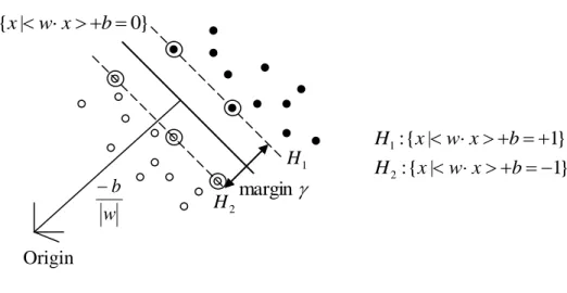
Figure 3.1 Linear separating hyperplanes for the separable case

As shown in Figure 3.1, the points x which lie on the hyperplanes satisfy

0

   

w x b , where w is normal to the hyperplane, b/ w is the perpendicular distance from the hyperplane to the origin, and w is the Euclidean norm of w. For the linearly separable case,

the support vector algorithm looks for the separating hyperplane with the largest margin.

Suppose that all the training data meet the following constraints.

1    x b w _i for y_i 1 (3.1) 1    x b w _i for y_i 1 (3.2) The margin  is defined as distance between two hyperplanes, H₁:wx_ib1 and

1 :

2 wx b

H _i with a normal w. Since these two hyperplanes are parallel and have the same

normal, the margin distance that separates them is given by Origin } 0 | {xwxb } 1 | { : 1 x wxb H } 1 | { : 2 x wxb H w b  margin _ 1 H 2 H





Each instance that falls on one of the two hyperplanes is called a support vector (SV).

The SVs in Figure 3.1 are circled. Given this geometric relationship, finding the hyperplanes

with the maximum margin in feature space can be formulated as a mathematical programming

problem. For a linearly separable training data S((x₁,y₁),....,(x_l.y_l)), the hyperplane producing

maximum margin is found by formulating the minimization optimization problem as follows:

,...., 1 , 1 ) ( subject to 2 / minimize 2 l i b x w y w i i       (3.4)

We now switch to a Lagrangian formulation of the problem with the Lagrange

multipliers,_i 0 . By doing this, the constraints in Equation (3.4) are replaced by constraints on the Lagrangian multiplier themselves, which are easier to handle. The primal Lagrangian is given

by



Then we must minimize L_P(w,b,) with respect to w and b, subject to i 0 . This is a convex quadratic programming problem since the objective function is itself convex, and those

points which satisfy the constraints also form a convex set. This indicates that this problem can

be equally solved with its corresponding dual problem, subject to the derivatives of L_P(w,b,) with respect to w and b,









also subject to the constraints, i 0 . Since these are equality constraints in the dual formulation, the dual can be substituted (3.6) into (3.5) and results in

. 2 1 2 1 ] 1 ) ( [ 2 1 ) , , ( 1 , 1 1 , 1 1 , 1 2













The primal (L_P) and dual (L_D) come from the same objective function but with different constraints and the solution is found by minimizing L_Por maximizing L_D. Given that we want to maximizeL_D with respect to i, the optimization problem can be formulated as

. ,...., 1 , 0 , 0 subject to 2 1 ) ( maximize 1 i 1 , 1 l i y x x y y L i l i i l j i j i j i j i l i i D        







In solving this problem, the positive values for each i gives



generates the maximal margin hyperplane with margin  1/ w* 2. Those points whose i is

positive are the SVs (and are located on H1 and H2 in Figure3.1), while other points‟i are zero.

Since the value of b does not appear in the dual problem, b*is found making use of the primal constraints. The optimal solutions * , (w*,b*) must satisfy

l i b x w y_{i i} i[ ( 1] 0, 1,..., * * *      

 . This is the Karush-Kuhn-Tucker (KKT)

complementary optimality condition. With this condition, b can be computed. The hyperplane

decision function can then be written as



This implies that support vectors are the critical points in the training set and lie closest to

the hyperplane producing the maximum margin of two different class labels.

So far we have considered only a separable case of training data. How can we extend

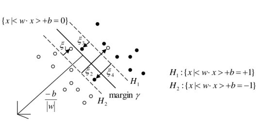
these strategies to deal with a non-separable case? This is done by introducing a positive slack

variable, i, i1,....,l. Constraints become:

i i b x w  1 for yi 1 (3.11) i i b x w  1 for yi 1 (3.12)

Figure 3.2 Linear separating hyperplanes for the non-separable case

So when an error occurs, the corresponding _i must exceed unity, so



i i is the upper

bound on the number of training errors. Hence a natural way to assign an extra cost for errors is

to change the objective function to be minimized from w2 /2 (see equation 3.4) to



 l

i i

C

w2/2 ₁ , where C is a penalty parameter chosen by the user. This is the concept behind

soft-margin SVMs. Introducing ias the Lagrange multipliers of the i, the Lagrange (primal)

function is:







For minimizing the Lagrange (primal) problem with respect to w, b, and i, setting the

respective derivatives to zero, we get equations (3.6) , (3.7) above, and

i C i i   ,   . (3.14) 4  2  3  1  } 1 | { : 1 x wxb H } 1 | { : 2 x wxb H } 0 | { x wxb  margin w b  1 H 2 H

By substituting the derivatives into the primal problem, the corresponding dual problem is formulated as . ,...., 1 , 0 , 0 subject to 2 1 ) ( maximize 1 i 1 , 1 l i C y x x y y L i l i i l j i j i j i j i l i i D         







With the derivatives and the KKT condition, equations (3.16)-(3.18), we obtain

0 } 1 ) ( { i i    i  i y x w b   (3.16) 0  i i  (3.17) 0 ) 1 ( ) ( _i    _i  i x w b y  (3.18)

The solution is given by



  Ns i i i iy x w 1

 , where Ns is the number of SVs which non-zero coefficient ˆ_i. Among the SVs, some lie on the edge of the margin (ˆ_i 0) that is characterized by 0ˆ_i C from equations (3.17) and (3.14) and the remaining (ˆ_i 0 ) have ˆ_i C . Therefore, points on the wrong side of the boundary are SVs and points on the correct side of the

boundary are also SVs.

A SVM is a linear classifier, but in most cases, it is practically restrictive. SVM can be

easily extended to a nonlinear classifier by mapping the input space into a high dimensional

feature space through a kernel function, K(x_i,x_j) which computes the dot product of the data

points in the feature space H, that is,

) ( ). ( ) , (x_i x_j x_i x_j K   . (3.19)

Functions that satisfy Mercer‟s theorem (Burges, 1998) can be used as dot products and thus can be used as kernels. Common kernel functions include Linear: K x x( ,_{i j})(x x_i _j), Polynomial:

( ,_{i j}) ( _{i j} 1)d

K x x  x x  and GaussianRadial-based:

2 2 2 / ) , ( xi xj  j i x e x K    .

Thus the nonlinear separating hyperplane can be found formulated as an optimization problem given by . ,...., 1 , 0 , 0 subject to ) ( 2 1 ) ( maximize 1 i 1 , 1 l i C y x x K y y L i l i i l j i j i j i j i l i i D       







The corresponding decision function is



3.2 SVMs and the Skewed Boundary

As noted previously, imbalanced data sets cause a bias in the results of a SVM. Akbani et

al. (2004) have summarized three reasons why a skewed boundary occurs in SVM classification

for imbalanced data sets: (1) positive (minority) instances lie further from the ideal boundary

compared with negative (majority) instances, (2) the weakness of the soft-margin SVMs and (3)

the imbalanced SV ratio. For the third reason, according to the KKT conditions in solving the

optimization problem in SVM, the values for imust satisfy ₁ 0 n

i i i y 



dominated by majority SVs. That means that the decision function is more likely to classify a

boundary as majority. The second reason, the weakness of the soft-margin SVMs, is an inherent

weakness in coping with imbalanced data learning. For separable cases, the imbalance of class

distribution rarely influences the performance of SVMs because all the slack variables iare

equal to zero (equations 3.11 and 3.12). Therefore, there is no contradiction between the capacity

of the SVMs and the classification error. However, for non-separable cases, soft-margin SVMs

should achieve a trade-off between maximizing the margin between two classes and minimizing

the classification error. Typically much more majority instances appear in the overlapping area

than minority ones. So, the optimal hyperplane will be skewed on the minority class side in order

to reduce the overwhelming errors of misclassifying the majority class. If C is not very large,

SVMs simply predict most of minority instances as majority instances to make the margin as

large as possible, making the total misclassification cost as small as possible.

Several methods for SVMs for imbalanced data learning have been studied (Karakoulas

& Taylor, 1999; Lin et al., 2002). At the data level, rebalancing approaches such as

over-sampling (i.e. SMOTE) and under-over-sampling have been widely used for SVM to cope with

imbalanced datasets. Veropoulos et al. (1999) suggested using different penalties for

misclassification of the classes. Amari and Wu (1999) proposed using conformal transformation

of the kernel matrix to enlarge the separation between two classes. In the first step, it finds the

separating location between two classes through standard SVM learning. In the second step, the

primary kernel matrix is conformally scaled to give a wider separation. Separation is controlled

by the SVs, so the new kernel matrix is enlarged at the position of SVs.

Another approach is the one-class SVM (Scholkoft and Smola, 2002). This uses only

of the data within a dataset. This determines a hyperplan in feature space that separates most of

the data from the origin. It completely ignores information of the majority class: Instead, only

using one class, the minority class , it defines a hyperplane that separates most of data belonging

to the class from the origin.

3.3 Problems associated with SVM classifier for imbalanced data

When focusing on approaches at the data level (rebalancing the data distribution), there

are two significant problems associated with a SVM classifier, namely,

1. Over-sampling methods significantly increase the dataset size.

2. An optimal ratio of class distribution is empirically determined by grid search.

To address these problems, we propose a new sampling method at the data level for

imbalanced data learning. Instead of rebalancing the entire imbalanced dataset, a selective

sampling method is proposed that results in a relatively small number of instances. We expect

that a small set of representative instances of an imbalanced dataset could determine the desired

decision boundary by maintaining the same or achieving even better performance for the class

imbalance problem as compared to existing rebalancing methods. The merits of this approach

include: (1) skipping empirical search that is necessary in sampling methods such as optimal

ratios of class distributions and (2) avoiding producing a large training set that would lead to

long training times for a SVM. If this approach performs well as compared to some current

methods, it will provide an alternative method to solve the class imbalance problem with the

3.4 Effectiveness of rebalancing class distribution

For imbalanced and highly overlapped class data, sampling methods such as

over-sampling or under-over-sampling are very effective in terms of the optimization process in a

soft-margin SVM. In order to illustrate the effect of sampling methods in rebalancing class

distribution, we examine the boundary movement in two common methods, SMOTE

over-sampling and Random under-over-sampling. In this example, a Gaussian kernel function is used for

SVM classification.

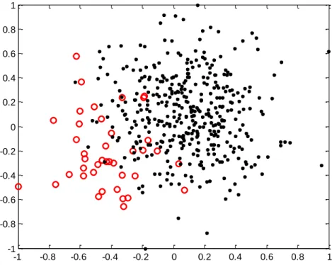
First, we generated a simple structure of a synthetic dataset showing a typical class

imbalance problem, which could be represented in 2-dimensional space as shown in Figure 3.3.

The minority class having 40 instances is marked with „o‟ and the majority having 400 instances

with „•‟ (a class ratio of 1:10).

-1 -0.8 -0.6 -0.4 -0.2 0 0.2 0.4 0.6 0.8 1 -1 -0.8 -0.6 -0.4 -0.2 0 0.2 0.4 0.6 0.8 1

After classification, almost all majority instances were correctly classified, while many

minority instances were classified as the majority class. This example illustrates a typical class

imbalance problem caused by soft-margin SVM algorithms. In other words, an optimal

hyperplane results from the trade-off between maximizing the margin of the minority and the

majority class and minimizing misclassification costs in the feature space. To improve the

accuracy for the minority class, we need to move the boundary toward the majority class side. To

illustrate this, we applied two rebalancing sampling methods, SMOTE and random

under-sampling, which will be referred to as SVM-SMOTE and SVM-RU, respectively.

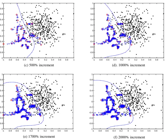
Using SVM-SMOTE, the number of synthetic instances to achieve the desired class

balance is unknown and empirical studies must be performed. Minority instances are

oversampled gradually with 100%, 300%, 500% and 1000% increases in minority instances.

After rebalancing by SMOTE, we observed that the boundary gradually shifted toward the

majority class as minority instances are increased as shown in Figure 3.4 (a) to (f).

-1 -0.8 -0.6 -0.4 -0.2 0 0.2 0.4 0.6 0.8 1 -1 -0.8 -0.6 -0.4 -0.2 0 0.2 0.4 0.6 0.8 1 -1 -0.8 -0.6 -0.4 -0.2 0 0.2 0.4 0.6 0.8 1 -1 -0.8 -0.6 -0.4 -0.2 0 0.2 0.4 0.6 0.8 1

-1 -0.8 -0.6 -0.4 -0.2 0 0.2 0.4 0.6 0.8 1 -1 -0.8 -0.6 -0.4 -0.2 0 0.2 0.4 0.6 0.8 1 -1 -0.8 -0.6 -0.4 -0.2 0 0.2 0.4 0.6 0.8 1 -1 -0.8 -0.6 -0.4 -0.2 0 0.2 0.4 0.6 0.8 1 -1 -0.8 -0.6 -0.4 -0.2 0 0.2 0.4 0.6 0.8 1 -1 -0.8 -0.6 -0.4 -0.2 0 0.2 0.4 0.6 0.8 1 -1 -0.8 -0.6 -0.4 -0.2 0 0.2 0.4 0.6 0.8 1 -1 -0.8 -0.6 -0.4 -0.2 0 0.2 0.4 0.6 0.8 1

circle(○): minority instances, dot(•): majority instances, cross(+): synthetic instances by SMOTE

Figure 3.4 Boundary movements by SMOTE algorithm

Though SVM-SMOTE shifts the decision boundary, it comes at a penalty of increasing

the size of the dataset as mentioned in the previous section. Assume that Npis the number of the positive (minority) instances and Nnthe number of the negative (majority) instances, typically

SVM takes O Np(( Nn) )3 time for learning in the worst case (Burges, 1998). For imbalanced

data learning, SVM-SMOTE will take O Np((  (1 Rsmote)Nn) )3 where Rsmoteis an optimal ratio

(c) 500% increment (d). 1000% increment

of size of increasing instances. Here Rsmoteis determined empirically. What is worse,

over-sampling also increases instances in the complex region between classes. By generating

instances near or in overlapping areas which might be misclassified, classification is more

difficult. In solving the optimization problem in the SVM algorithm, many cases can violate

KKT conditions. As a result, this will requires much more time to convergence of optimization

in SVM algorithms in spite of its good performance. So, if a dataset is extremely imbalanced and

overlapped, over-sampling through the SMOTE algorithm would not be efficient. In regard to

the problems introduced by an over-sampling approach, an under-sampling method is preferred

to over-sampling methods and is commonly used.

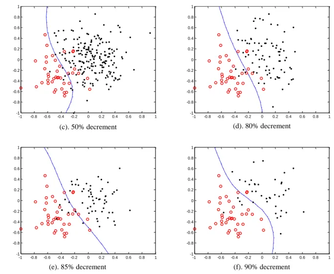
SVM-RU uses random under-sampling to rebalance the class distribution. Instead of

increasing minority instances, decreasing the number of the majority instances will make an

optimal hyperplane in terms of the trade-off between maximizing the margin and minimizing

misclassification costs. Figure 3.5 below shows the boundary movement as the number of the

majority instances removed randomly is increased.

-1 -0.8 -0.6 -0.4 -0.2 0 0.2 0.4 0.6 0.8 1 -1 -0.8 -0.6 -0.4 -0.2 0 0.2 0.4 0.6 0.8 1 -1 -0.8 -0.6 -0.4 -0.2 0 0.2 0.4 0.6 0.8 1 -1 -0.8 -0.6 -0.4 -0.2 0 0.2 0.4 0.6 0.8 1

-1 -0.8 -0.6 -0.4 -0.2 0 0.2 0.4 0.6 0.8 1 -1 -0.8 -0.6 -0.4 -0.2 0 0.2 0.4 0.6 0.8 1 -1 -0.8 -0.6 -0.4 -0.2 0 0.2 0.4 0.6 0.8 1 -1 -0.8 -0.6 -0.4 -0.2 0 0.2 0.4 0.6 0.8 1 -1 -0.8 -0.6 -0.4 -0.2 0 0.2 0.4 0.6 0.8 1 -1 -0.8 -0.6 -0.4 -0.2 0 0.2 0.4 0.6 0.8 1 -1 -0.8 -0.6 -0.4 -0.2 0 0.2 0.4 0.6 0.8 1 -1 -0.8 -0.6 -0.4 -0.2 0 0.2 0.4 0.6 0.8 1

Figure 3.5 Boundary movements by random under-sampling

Similar with SVM-SMOTE, random under-sampling causes a shift in the decision

boundary towards the majority class. Considering time complexity in learning the dataset,

SVM-RU takes O Np(( Nn R _u) )3 which is quicker than SVM with the original training set since

u

Nn R is approximately equal to Nn . Because majority instances have been randomly eliminated, it may not be easy to determine an optimal size of training set for rebalancing. Also

(c). 50% decrement (d). 80% decrement

similar to SVM-SMOTE, the optimal desired class distribution for imbalanced data learning is

unknown and needs to be determined empirically

3.5 Hypotheses

Given the nature of imbalanced datasets as previously discussed, two hypotheses were

formulated to address effectiveness and efficiency issues in imbalanced data learning for SVMs.

Hypothesis 1

A relatively small number of instances from an imbalanced training set are needed to obtain good performance in solving the class imbalance problem using a SVM.

Hypothesis 2

A smaller subset within the set of support vectors can be found that produces a better boundary using a SVM.

Hypothesis 1 is related to the premise that the boundary between the major and minor

classes is strongly influenced by a relatively small number of instances. The inference is that a

potential down-sizing of learning sets will lead to significant improvements in classifier

performance. Hypothesis 2 is based on the expectation that there is a smaller group of SVs that

will provide a near optimal classification of the classes and improve the efficiency of learning. If

such a set of SVs exist, then a metaheuristic-based sampling approach could be used to select the

CHAPTER 4 SELECTIVE SAMPLING USING A GENETIC ALGORITHM

This chapter presents a selective sampling method based on a Genetic Algorithm for

imbalanced data learning with a SVM. Instead of rebalancing new training data distributions for

learning, we investigate how this selective sampling method performs on class imbalance

problems. Instance selection is a form of under-sampling in which specific instances are selected

based on some criteria. We use a Genetic Algorithm to perform selective sampling of the

majority instances and retain all minority instances because they are assumed to be informative.

4.1 SVMs for Large-Scale Datasets

Training a SVM involves solving a constrained quadratic programming (QP) problem,

requiring a large memory allocation and resulting in long training times for large-scale data. Two

issues in using SVMs with large scale data are the generation of the kernel matrix and data

overlapping. With a dataset size of N, an N×N kernel matrix is generated. Furthermore, storing

the entire kernel matrix in memory is problematic due to computer memory limitations. The

second issue is the increase in classification difficulty when many class data are overlapped.

Due to large-scale data problem associated with SVMs, many studies have examined

methods for reducing training samples to achieve relatively fast SVM classification. For

example, Shin and Cho (2003) proposed a selection method for selecting patterns from training

data near the decision boundary based on the neighborhood properties. Zhang and King proposed

a -skeleton algorithm to identify SVs. Almeida et al. (2000) employed K-means clustering to select patterns from a training set. Lee and Mangasarian (2001) selected a subset of training