Knowl
edge
Engi
neeri
ng
Efficient Pairwise
Multilabel Classification
DissertationEneldo Loza Mencía
Knowledge Engineering Group Technische Universität Darmstadt [email protected]
Vom Fachbereich Informatik der Technischen Universität Darmstadt zur Erlangung des akademischen Grades eines Doktors der Naturwissenschaften (Dr. rer. nat.)
genehmigte
Dissertation
von
Diplom-Informatiker Eneldo Loza Mencía aus Frankfurt am Main
Referent: Prof. Dr. Johannes Fürnkranz Korreferent: Prof. Dr. Eyke Hüllermeier
(Philipps-Universität Marburg) Tag der Einreichung: 11. Juni 2012
Tag der Verteidigung: 24. Juli 2012
Darmstadt 2013 D17
Efficient Pairwise Multilabel Classification
Genehmigte Dissertation von Eneldo Loza Mencía aus Frankfurt am Main 1. Referent: Prof. Dr. Johannes Fürnkranz
2. Referent: Prof. Dr. Eyke Hüllermeier Weitere Prüfer:
Prof. Dr. Michael Goesele (Vorsitzender der Prüfungskommission) Prof. Dr. Chris Biemann
Prof. Dr. Thorsten Strufe
Tag der Einreichung: 11. Juni 2012 Tag der Verteidigung: 24. Juli 2012 Darmstadt, 2013 – D17
Bitte zitieren Sie dieses Dokument als Please cite this document as
URN: urn:nbn:de:tuda-tuprints-32260
URL: http://tuprints.ulb.tu-darmstadt.de/3226
Dieses Dokument wird bereitgestellt von This document is provided by
tuprints, E-Publishing-Service of the TU Darmstadt http://tuprints.ulb.tu-darmstadt.de
Die Veröffentlichung steht unter folgender Creative Commons Lizenz: This publication is licensed under the following Creative Commons license: Namensnennung – Nicht kommerziell – Keine Bearbeitung 3.0 Deutschland Attribution – Non-commercial – No Derivative Works 3.0 Germany
(CC BY-NC-ND 3.0 DE)
Kurzfassung
Multilabel-Klassifizierung bezeichnet die Aufgabe, eine Zuordnung von Objekten zu Men-gen von möglicherweise sich überlappender Klassen zu lernen. Dieses Feld hat in letzter Zeit stark an Aufmerksamkeit gewonnen. Ein praktisches Anwendungsszenario wäre die Zuweisung von Schlüsselwörtern zu Dokumenten. Ein Problem, das häufig im Gebiet der Text-Klassifizierung anzutreffen ist. Durch die aufkommenden Web 2.0 Technologien wird dieses Gebiet um eine Reihe von Szenarien erweitert welche sich hauptsächlich mit dem Empfehlen von Tags und Schlagwörtern konzentrieren. Der Trend geht dabei unausweichlich zu noch mehr Datenpunkten und noch mehr Labels. Die vorliegende Ar-beit bietet eine umfassende Einleitung in das Thema Multilabel-Klassifizierung mit einer detaillierten Formalisierung und einer ausführlichen Erläuterung der aktuellen Verfahren, die den Stand der Technik repräsentieren.
Ein gängiges Verfahren, um Multilabel-Probleme zu lösen, stellt die Zerlegung des Orig-inalproblems in mehrere Teilprobleme dar. Diese Teilaufgaben sind üblicherweise leicht mit konventionellen Techniken zu lösen. Im Vergleich zu der direkten Methode, dem Ler-nen eines Klassifizierers pro Klasse, der dann für jede Klasse unabhängig von den anderen die Relevanz vorhersagt (Binary Relevance), legt diese Arbeit ihren Schwerpunkt auf den Ansatz der paarweisen Zerlegung. Hierbei wird eine Entscheidungsfunktion für jedes Paar von Klassen gelernt. Der Hauptvorteil dieser Methode, die Verbesserung der Qualität der Vorhersagen, steht allerdings im Gegensatz zum Hauptnachteil, nämlich der quadratis-chen Anzahl von Klassifizierern. Diese Anzahl berechnet sich in Abhängigkeit der Anzahl der Labels. Diese Dissertation stellt ein Framework von effizienten und skalierbaren Lö-sungen für die Verarbeitung von hunderten und sogar tausenden von Labels vor, die trotz der quadratischen Abhängigkeit verarbeitet werden können.
Wie sich herausstellt, kann das Trainieren eines paarweisen Ensembles von Klassifizier-ern in linearer Zeit geschehen. Der Unterschied zum simplen Binary Relevance (BR) Ver-fahren beträgt hierbei nur einen kleinen Faktor, der der durchschnittlichen Zahl von as-soziierten Labels pro Objekt entspricht. Zusätzlich konnte durch die Anwendung eines intelligenten und dynamischen Auswertungsschemas, inspiriert durch das System der Sport-Ligen, die quadratische Anzahl an Auswertungen von Basis-Klassifizierern auf eine in der Praxis log-lineare Abhängigkeit reduziert werden. Die Kombination mit einem einfachen aber schnellen und mächtigen linearen Klassifizierer erlaubte die Echtzeit-Verarbeitung von Daten mit sehr vielen, hoch-dimensionalen Datenpunkten. Eine Auf-gabenstellung, die davor dem paarweisen Lernen nicht zugänglich war.
Der verbleibende Flaschenhals, die explodierenden Speicheranforderungen, wurde durch die Ausnutzung einer interessanten Eigenschaft von linearen Klassifizierern über-wunden, nämlich die Möglichkeit der dualen Reformulierung als Linearkombination der Trainingsbeispiele. Die Tauglichkeit dieses Verfahrens wurde auf dem neuartigen
TextdatensatzEUR-Lex demonstriert, welches insbesondere die Skalierbarkeit des paar-weisen Ansatzes auf die Probe stellt. Mit seinen fast 4.000 Labels und 20.000 Doku-menten stelltEUR-Lex eine der anspruchsvollsten Testdatensätze für Multilabel-Lernen dar. Die duale Formulierung ermöglicht es, ein Modell im Speicher zu halten, welches den 8 Millionen Basislernern, die bei der konventionellen Lösung für EUR-Lex nötig wären, entspricht, und das bei gleichen Speicherbedarf wie Binary Relevance. Darüber hinaus wurde BR in den Experimenten klar geschlagen. Ein weiterer Beitrag dieser Ar-beit, basierend auf einer hierarchischen Zerlegung und Anordnung der Originalaufgaben-stellung, ermöglicht sogar die Reduzierung der Abhängigkeit von der Anzahl der kleiner als linear. Dieser Ansatz öffnet einer großen Auswahl an neuen Herausforderungen und Anwendungen die Türen, aber es werden dabei auch die Vorteile des paarweisen Lernens beibehalten, nämlich die exzellente Qualität der Vorhersagen. Im Vergleich mit dem kon-ventionellen, flachen Ansatz konnte sogar gezeigt werden, daß sich bei Problemen mit vielen Labels ein besonders positiver Effekt beim Ausbalancieren von Recall und Precision einstellt.
Die verbesserte Skalierbarkeit und Effizienz ermöglichte es, den paarweisen Ansatz auf eine Menge von großen Multilabel-Problemen anzuwenden, die alle eine gemein-same, parallele Datenbasis aber unterschiedliche Domänen von Labels besitzen. Dieses Szenario von parallelen Tasks stellt einen ersten Schritt dar, die Fähigkeiten des paar-weisen Ansatzes für die Ausnutzung von Label-Abhängigkeiten zu untersuchen, mit ersten vielversprechenden Ergebnissen. Die Verwendung von Multilabel-Verfahren für die automatische Annotation von Texten stellt eine weitere offensichtliche, aber bislang verkannte Verbindung zu Multi-Task und Multi-Target-Learning dar. In der vorgeschlage-nen Lösung wird das gleichzeitige Markierung von Wörtern mit unterschiedlichen aber möglicherweise überlappenden Annotationsschemata als Multilabel-Problem betrachtet. Dieser Ansatz wird voraussichtlich von Verfahren, die Label-Abhängigkeiten berücksichti-gen, profitieren können. Die Fähigkeit des paarweisen Ansatzes hierfür ist klarerweise auf paarweise Relationen beschränkt. Deshalb wird in dieser Arbeit eine Technik untersucht, die Konstellationen von Labels erforscht, die nur lokal in Untergruppen der Datenpunkte zu finden sind. Zusätzlich zu dem festgestellten positiven Effekt dieser zusätzlichen In-formationen bietet die experimentelle Auswertung auch interessante Erkenntnisse über das unterschiedliche Verhalten von aktuellen Verfahren bezüglich der Optimierung und besonderen Bevorzugung von Multilabel-Evaluationsmaßes, ein kontroverses Thema im Gebiet der Multilabel-Klassifizierung.
Abstract
Multilabel classification learning is the task of learning a mapping between objects and sets of possibly overlapping classes and has gained increasing attention in recent times. A prototypical application scenario for multilabel classification is the assignment of a set of keywords to a document, a frequently encountered problem in the text classification domain. With upcoming Web 2.0 technologies, this domain is extended by a wide range of tag suggestion tasks and the trend definitely is moving towards more data points and more labels. This work provides an extended introduction into the topic of multilabel classification, a detailed formalization and a comprehensive overview of the present state-of-the-art approaches.
A commonly used solution for solving multilabel tasks is to decompose the original problem into several subproblems. These subtasks are usually easy to solve with conven-tional techniques. In contrast to the straightforward approach of training one classifier for independently predicting the relevance of each class (binary relevance), this work focuses particularly on the pairwise decomposition of the original problem in which a decision function is learned for each possible pair of classes. The main advantage of this approach, the improvement of the predictive quality, comes at the cost of its main dis-advantage, the quadratic number of classifiers needed (with respect to the number of labels). This thesis presents a framework of efficient and scalable solutions for handling hundreds or thousands of labels despite the quadratic dependency.
As it turns out, training such a pairwise ensemble of classifiers can be accomplished in linear time and only differs from the straightforward binary relevance approach (BR) by a factor relative to the average number of labels associated to an object, which is usually small. Furthermore, the integration of a smart scheduling technique inspired from sports tournaments safely reduces the quadratic number of base classifier evaluations to log-linear in practice. Combined with a simple yet fast and powerful learning algorithm for linear classifiers, data with a huge number of high dimensional points, which was not amenable to pairwise learning before, can be processed even under real-time conditions. The remaining bottleneck, the exploding memory requirements, is coped by taking advantage of an interesting property of linear classifiers, namely the possibility of dual reformulation as a linear combination of the training examples. The suitability is demon-strated on the novelEUR-Lextext collection, which particularly puts the main scalability issue of pairwise learning to test. With its almost 4,000 labels and 20,000 documents it is one of the most challenging test beds in multilabel learning to date. The dual formula-tion allows to maintain the mathematical equivalent to 8 million base learners needed for conventionally solvingEUR-Lexin almost the same amount of space as binary relevance. Moreover, BR was clearly beaten in the experiments.
A further contribution based on hierarchical decomposition and arrangement of the original problem allows to reduce the dependency on the number of labels to even sub-linearity. This approach opens the door to a wide range of new challenges and appli-cations but simultaneously maintains the advantages of pairwise learning, namely the excellent predictive quality. It was even shown in comparison to the flat variant that it has a particularly positive effect on balancing recall and precision on datasets with a large number of labels.
The improved scalability and efficiency allowed to apply pairwise classification to a set of large multilabel problems with a parallel base of data points but different domains of labels. A first attempt was made in this parallel tasks setting in order to investigate the ex-ploitation of label dependencies by pairwise learning, with first encouraging results. The usage of multilabel learning techniques for the automatic annotation of texts constitutes a further obvious but so far missing connection to multi-task and multi-target learning. The presented solution considers the simultaneous tagging of words with different but pos-sibly overlapping annotation schemes as a multilabel problem. This solution is expected to particularly benefit from approaches which exploit label dependencies. The ability of pairwise learning for this purpose is obviously restricted to pairwise relations, therefore a technique is investigated which explores label constellations that only exist locally for a subgroup of data points. In addition to the positive effect of the supplemental informa-tion, the experimental evaluation demonstrates an interesting insight with regards to the different behavior of several state-of-the-art approaches with respect to the optimization of particular multilabel measures, a controversial topic in multilabel classification.
Contents
1 Introduction 1
1.1 Challenges in Pairwise Multilabel Classification . . . 3
1.2 Contributions and Organization of the Work . . . 6
2 Fundamentals of Multilabel Classification 11 2.1 Input Object Space . . . 11
2.2 Classification Mapping . . . 11
2.3 Learning a Model and Predicting . . . 12
2.4 Output Label Space . . . 14
2.5 Types of Classification Problems . . . 15
2.5.1 Binary Classification . . . 15
2.5.2 Multiclass Classification . . . 17
2.5.3 Multilabel Classification . . . 17
2.5.4 Label Ranking . . . 19
2.5.5 Multilabel Label Ranking . . . 21
2.5.6 Hierarchical Classification . . . 22
2.6 Label Dependencies . . . 23
2.7 Evaluation Measures of Predictive Quality . . . 25
2.7.1 Aggregation and Averaging . . . 25
2.7.2 Cross Validation . . . 27
2.7.3 Bipartition Evaluation Measures . . . 27
2.7.4 Ranking Quality Measures . . . 31
2.7.5 Discussion . . . 35
2.8 Multilabel Learning Algorithms . . . 36
2.8.1 Transformational Approaches . . . 37
2.8.2 Holistic Approaches . . . 37
2.8.3 Generative Approaches . . . 38
2.8.4 Ensembles . . . 39
2.8.5 Instance Input Space Transformations . . . 40
2.8.6 Label Output Space Transformations . . . 40
2.8.7 Alternative Structures and Formulations . . . 41
2.9 Datasets and Application Scenarios . . . 42
2.9.1 Benchmark Datasets . . . 43
2.9.1.1 Text . . . 45
2.9.1.2 Multimedia . . . 46
2.9.1.3 Biology . . . 47
2.9.2 Sources and Repositories . . . 47
2.10 Statistical Comparison of Classifiers . . . 47
2.10.1 Sign Test . . . 48
2.10.2 Wilcoxon Signed-Ranks Test . . . 49
2.10.3 Friedman and Post-Hoc Tests . . . 50
3 Decompositive Approaches to Multilabel Classification 53 3.1 Binary Relevance Decomposition . . . 54
3.1.1 Computational Complexity . . . 56
3.2 Label Powerset Transformation . . . 57
3.2.1 Computational Complexity . . . 58
3.3 Error Correcting Output Codes . . . 58
3.4 Pairwise Multilabel Decomposition . . . 59
3.4.1 Decomposition . . . 59
3.4.2 Pairwise Preference Learning . . . 60
3.4.3 Aggregation . . . 61 3.4.4 Bipartitioning . . . 63 3.4.5 Calibration . . . 63 3.4.6 Computational Complexity . . . 65 3.4.6.1 Training . . . 66 3.4.6.2 Predicting . . . 67
3.4.6.3 Super-linear Base Learner . . . 68
3.5 Discussion . . . 70
3.5.1 Easier Subproblems . . . 70
3.5.2 Non-Competent Base Classifiers . . . 71
3.5.3 Instances in the Label Intersections . . . 71
3.5.4 Bipartitioning and Calibration . . . 73
3.5.5 Label Ranking . . . 74
3.5.6 Aggregation and Voting . . . 77
3.5.7 Comparison to Binary Relevance Decomposition . . . 78
3.5.8 Comparison to Ternary ECOC . . . 80
3.5.9 Summary: Advantages and Disadvantages . . . 81
4 Pairwise Learning of Efficient Perceptrons 83 4.1 Perceptrons . . . 84
4.1.1 Linear Classifiers . . . 85
4.1.2 Perceptron Training Rule . . . 85
4.1.3 Bias and Threshold . . . 86
4.1.4 Dual Form . . . 86
4.1.5 Maximum Margin Hyperplane and Problem Hardness . . . 87
4.1.6 Support Vector Machines . . . 87
4.1.7 Comparison . . . 88
4.3 Multiclass Multilabel Perceptrons . . . 90
4.4 Multilabel Pairwise Perceptrons . . . 91
4.5 Comparison . . . 92 4.5.1 Discussion . . . 92 4.5.2 Computational Complexity . . . 93 4.5.2.1 Memory Requirements . . . 94 4.5.2.2 Training . . . 95 4.5.2.3 Prediction . . . 95
4.5.2.4 Sparsity of Feature Vectors . . . 96
4.6 Evaluation . . . 96 4.6.1 Experimental Setup . . . 96 4.6.2 Ranking Quality . . . 98 4.6.3 Calibration Performance . . . 98 4.6.4 Computational Costs . . . 100 4.6.5 Learning Curve . . . 101 4.6.6 Overfitting Analysis . . . 102
4.6.7 Concept Drift Analysis . . . 102
4.6.8 Results on other Datasets . . . 104
4.6.9 Discussion on Cardinality Prediction . . . 107
4.7 Summary . . . 108
5 Efficient Aggregation Strategies 111 5.1 Quick Weighted Voting . . . 112
5.1.1 QVoting for Multiclass Classification . . . 113
5.1.2 QVoting for Multilabel Classification . . . 114
5.1.3 Extensions . . . 115 5.2 Computational Complexity . . . 116 5.3 Experimental Setup . . . 117 5.3.1 Datasets . . . 117 5.3.2 Algorithmic Setup . . . 117 5.4 Evaluation . . . 118 5.4.1 Computational Efficiency . . . 120 5.4.2 Predictive Quality . . . 123
5.4.3 Support Vector Machines . . . 124
5.5 Discussion and Related Work . . . 126
5.6 Summary . . . 127
6 Highly Scalable Dual Models 129 6.1 The EUR-Lex Repository . . . 130
6.1.1 Retrieval . . . 132
6.1.2 Statistics . . . 132
6.1.3 Preprocessing . . . 136
6.2 Dual Multilabel Pairwise Perceptrons . . . 136
6.2.1 Calibration . . . 138
6.2.2 Discussion and Further Extensions . . . 139
6.3 Computational Complexity . . . 140 6.3.1 Memory Requirements . . . 141 6.3.2 Training . . . 142 6.3.3 Predicting . . . 142 6.4 Evaluation . . . 143 6.4.1 Experimental Setup . . . 143 6.4.2 Ranking Quality . . . 143
6.4.3 Bipartition Prediction Quality . . . 145
6.4.4 Computational Costs . . . 146
6.4.4.1 Training and Prediction Costs . . . 147
6.4.4.2 Memory Costs . . . 149
6.5 Related Work . . . 150
6.6 Summary . . . 151
7 Hierarchical Model Efficiency and Scalability 153 7.1 HOMER: Hierarchy of Multilabel Classifiers . . . 154
7.1.1 Training . . . 154 7.1.2 Predicting . . . 155 7.1.3 Hierarchy Construction . . . 155 7.2 Computational Complexity . . . 156 7.2.1 Memory . . . 157 7.2.2 Training . . . 157 7.2.3 Predicting . . . 159 7.3 Evaluation . . . 159 7.3.1 Setup . . . 160
7.3.2 Results of HOMER with QCLR . . . 160
7.3.2.1 Training Time . . . 161
7.3.2.2 Testing Time . . . 161
7.3.2.3 Predictive Quality . . . 163
7.3.3 Comparison of HOMER against its Base Classifiers . . . 165
7.3.3.1 Predictive Quality . . . 165
7.3.3.2 Computational Time . . . 167
7.4 Related Work and Discussion . . . 168
7.5 Summary . . . 169
8 Exploitation of Label Dependencies in Parallel Tasks 171 8.1 Related Work . . . 172
8.2 Preliminaries . . . 173
8.3 Parallel Task Learning . . . 173
8.3.2 Calibration . . . 175 8.3.3 HOMER with QCLR . . . 175 8.4 Datasets . . . 177 8.5 Evaluation . . . 178 8.5.1 Additional Experiments . . . 181 8.6 Summary . . . 181
9 High-Order Dependencies with Patterns from Subgroup Discovery 183 9.1 Preliminaries . . . 184
9.1.1 The LeGo Framework . . . 184
9.1.2 Multilabel Classification . . . 185
9.1.3 Problem Statement . . . 187
9.2 Local Pattern Discovery Phase . . . 187
9.2.1 Exceptional Model Mining . . . 187
9.2.2 Exceptional Model Mining meets Bayesian Networks . . . 188
9.3 Pattern Subset Discovery Phase . . . 190
9.4 Global Modeling Phase . . . 191
9.5 Experimental Setup . . . 192
9.5.1 Datasets and Learners . . . 192
9.5.2 Obtaining Raw Results . . . 192
9.6 Evaluation . . . 193
9.6.1 Feature Selection Methods . . . 194
9.6.2 Evaluation of the LeGo Approach . . . 194
9.6.3 Evaluation of the Decompositive Approaches . . . 197
9.6.4 Efficiency . . . 198
9.7 Discussion and Related Work . . . 199
9.8 Summary . . . 200
10 Information Extraction and Syntactic Parsing 203 10.1 Information Extraction . . . 204
10.1.1 Boundary Classification . . . 204
10.1.2 Feature Generation . . . 205
10.2 Multilabel Classification for Information Extraction . . . 205
10.3 Evaluation . . . 206
10.4 Related Work . . . 207
10.5 Summary . . . 208
11 Summary and Conclusions 209 11.1 Challenges Revisited . . . 209
11.2 Perspectives . . . 211
11.3 Conclusions . . . 212
Bibliography 213
Own Publications 241
Acknowledgments 245
Curriculum Vitae 247
List of Figures
1.1 Schematic complexity diagram for multiclass classification . . . 5
2.1 Taxonomy of problem settings . . . 18
2.2 Examples of multipartite label ranking . . . 21
2.3 Diagrams of predicted label rankings and measures . . . 31
3.1 Subproblems in binary relevance multilabel classification . . . 55
3.2 Subproblems in pairwise multilabel classification . . . 59
3.3 Pairwise multilabel training . . . 61
3.4 Pairwise voting table . . . 63
3.5 Calibrated pairwise multilabel training . . . 64
3.6 Pairwise voting table with calibrated label . . . 64
4.1 Subproblems in the multiclass multilabel perceptrons approach . . . 89
4.2 Pseudocode of the MMP algorithm . . . 90
4.3 Pseudocode of the training method of the MLPP algorithm . . . 91
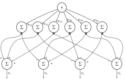
4.4 MLPP ensemble as neural network . . . 93
4.5 Predicted and actual number of classes onrcv1 . . . 99
4.6 Recall/Precision and ROC curves onrcv1 . . . 100
4.7 Learning curve for the full dataset . . . 102
4.8 Error on training and test data depending on the number of epochs . . . . 102
4.9 Comparison of random decision trees and CMLPP on driftedrcv1 . . . 105
4.10 Learning curve of CMLPP on driftedrcv1 . . . 105
5.1 Pseudocode of the QVoting algorithm . . . 113
5.2 Pseudocode of the QCLR2 aggregation algorithm . . . 114
5.3 Prediction complexity of QVoting and QCMLPP . . . 121
5.4 Prediction complexity of QCMLPP . . . 122
6.1 Excerpt of aEUR-Lex sample document . . . 131
6.2 Visualization of the EUROVOC graph. . . 133
6.3 Distribution of the labelset sizes for the threeEUR-Lexdatasets . . . 134
6.4 Diagram of the sizes of the labels onEUR-Lex . . . 135
6.5 Distribution of the sizes of the labels onEUR-Lex . . . 135
6.6 Pseudocode of the incremental training method of the DMLPP algorithm . 138 6.7 Pseudocode of the prediction phase of the DMLPP algorithm . . . 139
7.1 Hierarchy of a HOMER classifier . . . 155
7.2 Training time over number of partitions for the six HOMER variants . . . . 162
7.3 Testing time over number of partitions for the six HOMER variants . . . 162
7.4 Micro recall over number of partitions for the six HOMER variants . . . 164
7.5 Micro precision over number of partitions for the six HOMER variants . . 164
7.6 Micro F1 over number of partitions for the six HOMER variants . . . 165
8.1 Pairwise training on two separate tasks . . . 174
8.2 Pairwise training on the global task . . . 174
8.3 Calibration in the two separate tasks . . . 176
8.4 Calibration in the global task . . . 176
8.5 Joined calibration in the global task . . . 176
9.1 The LeGo framework . . . 184
9.2 Decomposition of multilabel training for BR, MC and LP . . . 186
9.3 Example Bayesian networks . . . 189
9.4 A MLC problem and its representation in pattern space . . . 191
10.1 Transformation of a text sentence into a classification problem . . . 203
10.2 Example of a syntax tree . . . 204
List of Tables
2.1 Classification type matrix . . . 15
2.2 Statistics of multilabel datasets . . . 44
3.1 Overview of transformation approaches and properties . . . 54
3.2 Complexity comparison . . . 66
3.3 Extended complexity comparison under idealistic assumptions . . . 68
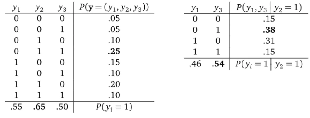
3.4 Example of joint and marginal probabilities . . . 75
4.1 Computational complexity of perceptron-based MLPP, BR and MMP . . . . 94
4.2 Comparison of CMLPP vs. others on thercv1 test set . . . 97
4.3 Comparison of the computational costs . . . 101
4.4 Comparison of CMLPP vs. others on others test sets . . . 106
5.1 Sports competition example . . . 112
5.2 Computational complexity comparison of the QVoting approach . . . 117
5.3 Statistics of datasets for the QVoting experiments . . . 118
5.4 Computational costs comparison to QVoting CLR . . . 119
5.5 Bipartitioning performance comparison to QVoting CLR . . . 124
5.6 Computational Costs for QCLR with SVMs . . . 125
5.7 Bipartitioning performance with SVM as base classifier . . . 126
6.1 Statistics of the EUR-Lex datasets . . . 132
6.2 Computational complexity of the perceptron based algorithms . . . 141
6.3 Average ranking losses on the EUR-Lex datasets . . . 144
6.4 Average bipartitioning losses on the EUR-Lex datasets . . . 146
6.5 Computational costs on the EUR-Lex datasets . . . 147
6.6 Memory requirements for theEUR-Lexdatasets . . . 149
7.1 Complexity comparison of BR and CLR combined with HOMER . . . 158
7.2 Dataset statistics for the HOMER experiments . . . 160
7.3 Bipartition measures and computational costs for HOMER . . . 166
8.1 Statistics for datasets for parallel tasks experiments:EUR-lex andrcv1 . . 177
8.2 Statistics for datasets for parallel tasks experiments:hifind . . . 178
8.3 Results of DCMLPP on theEUR-Lexdataset, parallel tasks . . . 179
8.4 Results of HOMER on thehifind dataset, parallel tasks . . . 180
8.5 Results of MLPP on thercv1 dataset, parallel tasks . . . 180
9.1 Datasets used in the subgroup discovery experiments . . . 192
9.2 Average ranks of different feature selection methods . . . 193
9.3 Comparison of different feature sets . . . 195
9.4 Comparison of the different base learners . . . 196
9.5 Comparison of the different decomposition approaches . . . 197
1 Introduction
It is a human necessity to comprehend and organize the environment. Hence, things in the real world are often analyzed, characterized, described, collected, archived, ordered, grouped and catalogued. One of the most studied objects are writings. Libraries of texts on papyrus in Ancient Egypt are known to have existed more than a thousand years BC. Even in these early antique collections, the writings were ordered or grouped according to certain characteristics. Nowadays, we find books ordered according to authors, titles, publication years, languages etc., and classified into genres, topics, subjects and so on.
These assignments were usually made by humans. The aim ofMachine learning is to provide tools and algorithms which facilitate an automatic machine-driven assignment. Learning or classification algorithms e.g.learnfrom previously seen assignments ofclasses
to objects and aim at using this “experience” for the automaticclassificationof new, un-seen objects. Such things or objects in this context are often also referred to asexamples
orinstances. Objects that are used to learn are commonly calledtrainingexamples, and
an automatic classification orpredictionis done on atestexample.
A classic exercise in machine learning is multiclass classification. The task consists in learning an assignment of objects to one class in a set of alternatives. Returning to our library example, the possible classes could be genre labels such asfiction,literature,
ro-mance,crime etc. Multiclass classification is very well studied and many solutions have
been developed for this problem. In recent years however, a related task has gained in-creased attention:Multilabel classificationassumes that classes are not necessarily disjoint and, hence, that a thing can be assigned to multiple classes simultaneously. The given ex-ample of the list of genres indeed seems to indicate that this is not an exceptional but rather the usual case.
However, the limited degree of previous research on multiclass problems had very concrete reasons. Firstly, available catalogs often did not allow multiple assignments. This ensured simplicity and hence efficiency (e.g. in locating books) on the one hand and effectivity (no copies needed, see below) on the other. Classification systems with elaborated topic hierarchies were specifically developed in order to prevent multiple as-signments. In the exceptional case that amultilabelassignment was needed, things were either assigned to the most descriptive, fitting class, or they were just replicated and then put into several classes. If multiple assignments could not be avoided, separate classifi-cation system were defined according to orthogonal facets, with one facet serving as the main one. Secondly, the practical and self-imposed restriction to the multiclass case in the past considerably helped the research community to understand some of the general foundations of learning algorithms. Moreover, the available resources, both in terms of data and computationally, were restricted.
With the rise of electronically available information and the “digital revolution of infor-mation society”, most of the stated classic limitations have become unnecessary. The vast amount of electronically available data demands for new solutions and approaches since pure human classification has become impractical. A prototypical example for the new challenges and possibilities are the meanwhile ubiquitous participatory networks, the so called Web 2.0. They make it easy for a user to label “things” with keywords, without restrictions regarding the number of assignments to an item.
Efficient approaches are more than ever necessary in order to tackle this large amount of data. However, previous advances, especially regarding the accuracy of automatic clas-sification, should not be ignored.
One of these notable advances concerns the initial decomposition of the original task. The division into several tasks is a commonly applied technique in order to simplify the original problem so that it becomes amenable to existing learning approaches. The decomposition into one problem for each class is the oldest and simplest approach in machine learning: Aclassifier is learned to distinguish objects of one specific class from objects not belonging to this class, which is why it is usually called one-against-all. In
pairwise decomposition we learn classifiers that are able to distinguish two classes, i.e.
whether it belongs to one or to the other.
The approach of pairwise comparison was first scientifically investigated in 1927 by Thurstone in the context of psychology and the measurement of personal feelings and preferences. In machine learning, the first attempts encompass the works of Knerr et al. (1990) and since then the superiority to one-against-all was shown in several studies (cf. Section 3.5.7). Moreover, many machine learning software tools use pairwise decom-position as the default setting, including two popular implementations of the state-of-the-art support vector machines algorithm (Chang and Lin 2001, Witten and Frank 2005), so that we can expect that its use is wide-spread. The main reason for the advantage over one-against-all is, intuitively, that it is easier to learn to distinguish between two classes than between one and all of the remaining classes.
However, one obvious drawback of pairwise decomposition lies in the fact that a class has to be compared to each other class separately; hence a quadratic number of classi-fiers, with respect to the number of classes, is necessary. Fürnkranz (2002) showed that, surprisingly, it is more efficient in the multiclass setting to learn this quadratic number of classifiers than the linear number of classifiers needed for one-against-all. Still, applying the pairwise classifiers is more expensive than for the one-against-all approach.
Furthermore, it has not been clear to what extent these statements apply to the more complex multilabel classification setting. In face of the increased demands due to the explosion of available data, it is also not clear how classical techniques, and in particular pairwise learning, will behave. Of course, the hope is to be able to benefit from the impor-tant advantages and improvements of the pairwise approach even under these adverse circumstances. The main objective of this work shall thus be to investigate methods and techniques forefficient pairwise multilabel classification.
The next section will identify the main challenges in automatic classification and in particular in multilabel classification.
1.1 Challenges in Pairwise Multilabel Classification
Decomposition, and in particular pairwise decomposition, is a general approach for clas-sification that decomposes a global task into several sub-tasks which have to be solved with conventional algorithms and tools from machine learning. Therefore, the limitations and dependencies of the underlying solvers are commonly shared. In addition, new re-strictions arise from the particular method of the pairwise decomposition, namely from the explicit consideration of all possible pairs of classes.
The following enumeration will state the main challenges in pairwise multilabel clas-sification. We will see which problem variables of a multilabel problem may affect scala-bility, efficiency and predictive quality of the pairwise approach.
Without going into more formal details, we define efficiency as the processing speed in terms of objects per time and scalability as the ability of a learning approach to handle a growing quantity. We will generally consider the predictive quality separately from the aforementioned quantities. Obviously, scalability is bounded by efficiency, since if efficiency decreases with a growing variable, an approach has demonstrated its inability to scale. Thus, in our context of learning and classifying, scalability is mainly concerned with memory issues, since speed is already covered by efficiency.
We will commonly assume, without loss of generality, a task of learning and classifi-cation of multilabel texts since text problems frequently cover several of the following issues. However, our considerations are not limited to these fields, and in fact multilabel classification come up in applications as diverse as music classification, image, video and semantic scene classification and protein function classification (cf. Section 2.9.1).
• Dimensionality of input: the number of features
In classification, an object is described by a set of features and feature values, also called attributes and attribute values (cf. Section 2.1). A common representation for text e.g. is to indicate for each word (feature) the number of times it appeared in the text (value). Obviously, this could lead to very high number of features for vast document collections. Many learning algorithm are very susceptible to this quantity for different reasons. Decision trees and rule learners e.g. have to explore the space of the features since they rely on patterns of feature values. On the other hand, the classification costs are usually not affected so much, since the number of feature tests is relatively low. For other approach such as linear classifiers (cf. Section 4.1.1) the training costs are less controlled by the number of features, but instead the memory requirements.
Pairwise classification shares these dependencies on the number of features since it decomposes the original problem and has further to apply conventional approaches to the generated subproblems. Fortunately, several methods in machine learning aim at a pre-selection or reduction of features. They provide an effective way of keeping the influence on scalability and efficiency constant, so we will resort to these if necessary.
• Quantity of data: the number of examples
Particularly in the early days of machine learning, appropriate data for experimen-tation was costly and hence scarce. Nowadays, we face vast amounts of data, which is mainly reflected in the number of examples a particular database contains. A view on two collections available from the Reuters agency demonstrates this. While the first one, retrieved in 1987, contained a little bit more than 20,000 news arti-cles,1the second one already collected more than 800,000 documents in one year (beginning in August 1996, see Lewis et al. 2004). The Internet has also frequently served as a potentially infinite source for new classification benchmarks since then (cf. Section 2.9.1).
Learning algorithms behave very differently with respect to the number of data provided for training. Somesupport vector machines(cf. Section 4.1.6) implemen-tations e.g. have to compare each training example with all other training exam-ples, which makes them infeasible for the aforementioned cases. Lazy techniques also quickly become impractical, since they almost have zero training costs, but they must compare each test example to each training example during prediction. Moreover, both approaches have to maintain at least a part of the training data in memory. Hence, great care has to be taken at the time of selecting the appropriate base classifier and it is absolutely necessary to foresee possible limitations.
The increasing availability of data and hence the need for efficient processing was one of the main starting points of the present work. Since a reduction of the accel-eration of data growth cannot be expected, this issue remains a key challenge for the future.
• Availability of data: real-time processing
This point may be seen as a direct consequence of the previously discussed explo-sion of the availability of data. Part of the effort shall hence be dedicated to the investigation of approaches which enable processing of multilabel data with almost no or small delay. This includes the immediate consideration of new training exam-ples for successive predictions as well as the instantaneous classification of a new example in the sense that a prediction is not delayed by the continuous training. In machine learning, these two aspects are typically described asonlineorincremental
training (cf. e.g. Sebastiani 2002, Sec. 6.6) andanytimeclassification, respectively. • Dimensionality of output: the number of classes
In classification, the output usually refers to the prediction of a classifier and the number of alternatives that may be predicted is higher the more classes we have. Therefore, the number of classes is also a variable of great importance to multiclass classification.
1 This is the oldest multilabel dataset used in machine learning research known to the author (Hayes and Weinstein 1991, Lewis 1992, 2004). In the20-newsgroupsdataset postings may also belong to sev-eral folders, but the dataset was simplified to multiclass by replicating the instances (Mitchell 1997).
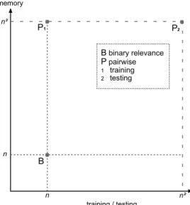
B n n n² n² B binary relevance P pairwise 1 training 2 testing training / testing memory P2 P1
Figure 1.1:Schematic complexity diagram comparing pairwise decomposition and one-against-all.
Training and testing (x-axis, sub-indices1and2, respectively, are used if not equal), memory (y-axis)
are shown with respect to the number of classesn.
But the output dimensionality plays the key role particularly in pairwise classifica-tion, since the number of classifiers which have to be learned quadratically depend on the number of possible classes. A few recent examples emphasize this: a dataset extracted from the social bookmarking page del.icio.ushad documents assigned to almost 1000 possible tags. And the EUR-Lex collection of official documents of the European Union presented in this work is indexed with a taxonomy contain-ing almost 4000 keywords. This would require a number of pairwise classifiers that reaches the magnitude of millions. Without adequate solutions such scenarios would definitively reach the boundaries of scalability and efficiency of the pairwise approach. The number of classes is therefore the main challenge for pairwise learning.
A schematic comparison of the distinct complexities of one-against-all and pairwise decomposition is shown in Figure 1.1. The diagram shows the dependence of the training and prediction costs (projection on the x-axis) and memory (y-axis) on the number of classesnfor multiclass problems. For multilabel problems, we can expect further movements to the upper-right corner, as we will see in the next paragraph. But the goal shall be to approach the bottom-left corner. A resolution including the solutions in this work will be given at the end of the work in Figure 11.1.
Two additional issues emerges from the fact that the multilabel setting allows as-signing an arbitrary number of labels to one instance. Firstly, and this is common to all multilabel solutions, dropping the multiclass restriction suddenly leads to ex-ponential grow of the number of alternatives. Whereas in multiclass classification the output space was the set of classes, it is the power set of the set of classes for
multilabel classification. This issue is alleviated by simplifying the task to predicting a ranking over the labels, but this entails further complications, as we will see in this work. Secondly, and this is specific to pairwise learning, the training efficiency is decreased since the costs grow with the possible combinations between true and false labels. In multiclass classification the number of combinations is always con-stant and approximately the number of classes, but in multilabel data the size of the correct labelset becomes arbitrary and the number of combinations grows ex-ponentially. The present work will also analyze in more detail this efficiency aspect. Note that the number of classifiers, and hence scalability and prediction efficiency, is not touched by this issue.
• Dependencies between the Labels
A point which clearly distinguishes multilabel from multiclass problems are the possible dependencies between the classes. Labels can co-occur or correlate with other labels and this might be an indication for certain dependencies. Imagine e.g. a book which was assigned to the keywordmurder. We could surely suspect that it was also annotated withcrime. Indeed, this relation could be imperative, but note that the opposite is not as probable.
A frequent concern in multilabel research from the beginning (for an early example, see McCallum 1999) is hence the modeling and exploitation of this additional data for producing more accurate results. This point will also be covered in this work, but to a smaller degree than our main issue of efficiency and scalability. The concern will rather be to investigate whether and to which degree the pairwise approach can exploit label dependencies under the constraints of high efficiency.
1.2 Contributions and Organization of the Work
In light of the stated demands and challenges of current and modern multilabel classifi-cation, this work makes the following main contributions:
• A general review of pairwise decomposition in multilabel classification is provided. • A new multilabel dataset is provided which is currently the most challenging bench-mark available in multilabel classification research due to the high dimensionality on the classes.
• A family of pairwise and combining learners is developed that provide the appro-priate instruments in order to respond to any combination of the stated challenges and demands on efficiency and scalability.
• The suitability of the frame is substantiated by a detailed formal and empirical investigation of the computational costs of the different decompositive approaches, particularly of the introduced pairwise learners.
The following listing shows the organization of the present work. A short summary is given for each chapter presenting further contributions which could not be reflected above in the condensed enumeration of the major contributions. In addition, significant parts of this thesis have previously appeared in publications of the author. The most relevant are accordingly indicated.
• Chapter 2
This chapter introduces concepts, notations and the corresponding basic formal def-initions required throughout this work. Furthermore, I discuss and review relevant existing and newly introduced evaluation measures, methods of comparison, prior learning approaches and the multilabel data available for research.
• Chapter 3
The basic decompositive approaches to multilabel classification are presented in Chapter 3. The formal analysis of the pairwise decomposition approach provides the basis for later analyses in this work. Critical aspects and limitations as well as advantages and disadvantages of the pairwise approach are discussed and summa-rized.
• Chapter 4
This chapter connects to the prior work of the author (Loza Mencía 2006, diploma thesis), which presented the efficientMLPPranking algorithm. MLPP is extended so as to incorporate calibration(Brinker et al. 2006), a new technique in the frame-work of pairwise preference learning which naturally enables to predict a set of labels. An extensive empirical study, the first of its sort, confirms the superiority of the pairwise approach, the suitability of calibration and the ability for real-time processing of a high quantity of data ofCMLPP.
– Loza Mencía and Fürnkranz 2008c
– Fürnkranz, Hüllermeier, Loza Mencía and Brinker 2008 • Chapter 5
CMLPP is naturally combined with the approach of QVoting(Park and Fürnkranz 2007) toQCMLPP(Loza Mencía et al. 2009), which is able to break the main lim-itation of the pairwise approach with respect to efficiency, namely the quadratic number of evaluations during prediction. It is demonstrated in a comprehensive empirical evaluation that it is possible to considerably improve this to a log-linear dependency on the number of classes. Moreover, the results show again the supe-riority over the competing decompositive approaches, regardless of the employed base learner (QCLR).
– Loza Mencía, Park and Fürnkranz 2009 – Loza Mencía, Park and Fürnkranz 2010 • Chapter 6
A vast collection of legal document from the European Union with a set of roughly
4000 classes is introduced in this chapter. Whereas this high number impeded employing pairwise decomposition in a first study (Loza Mencía and Fürnkranz 2007a), MLPP was subsequently reformulated to the mathematically identicalDual MLPP which enables scaling pairwise decomposition to the resulting 8 million classifiers. In contrast to MLPP, the pairwise base linear classifiers in DMLPP are represented in thedual as linear combination of the training examples instead of explicitly as a decision vector. The training set and the necessary coefficients eas-ily fit in memory in contrast to conventional MLPP. The dual variant substantially outperformed the baselines on theEUR-Lexdataset in terms of predictive quality.
– Loza Mencía and Fürnkranz 2007a – Loza Mencía and Fürnkranz 2008a – Loza Mencía and Fürnkranz 2010
• Chapter 7
The combination of QCLR with a hierarchically decomposing approach named HOMER (Tsoumakas et al. 2008) provides a more than suitable basis for even more challenging cases. HOMER decomposes the original problem into a hierarchy of considerably simpler multilabel problems, where each subproblem corresponds to a meta-label in the parent problem. The subproblems are then solved with QCLR. As it turns out, both approaches harmonize perfectly and the one-against-all base-line is again outperformed in terms of predictive quality, but also in training and testing efficiency, whereas the memory requirements only differ by a constant fac-tor. In contrast to DMLPP,H-QCLR’s formulation is not equivalent anymore, but the simplification preserves the positive effects of pairwise classification.
– Tsoumakas, Loza Mencía, Katakis, Park and Fürnkranz 2009b
• Chapter 8
This chapter describes a first attempt at exploiting label correlations with pairwise classifiers. It is shown that a globally trained classifier is superior to a locally trained one in a multilabel multi-task setting, which demonstrates the ability to exploit inter-label connections. The advances in the previous chapters prepared the ground for these experiments, since the multi-task setting multiplies the number of labels in the global problem.
– Loza Mencía 2010b
• Chapter 9
The issue of label dependencies is also the focus of this chapter, which describes a first investigation in order to connect conventional multilabel classification to local pattern discovery. Locally exceptional patterns in the labels are extracted and an empirical study shows the benefit of this approach, not only for pairwise decompo-sition.
• Chapter 10
The work described in this chapter is related to Chapter 8 but has information extraction and the common approach to learn each type of information separately as major concern.
– Loza Mencía 2010a
• Chapter 11
The last chapter summarizes the findings and results of the previous chapters. The big picture is drawn and the perspectives for possible future works are shown.
2 Fundamentals of Multilabel
Classification
Before we focus on the problem of multilabel classification, we have to state the general setting of a classification task in machine learning (Sections 2.1 to 2.4). The multilabel scenario is then demarcated from related types of problems in Section 2.5. Section 2.7.3 and 2.10 are dedicated to the evaluation and comparison of the prediction quality of multilabel classifiers, which we can train on the datasets presented in Section 2.9.1.
2.1 Input Object Space
In the field of machine learning,classificationdenotes the task of learning an association
of objects to classes in a supervised manner. An object may be anything, a document,
an image, person, etc. In order to being able to process the objects, we require that the object can be represented by a list of characteristics or attributes.2In particular, we will represent an instance or object as a vectorxof real-valued attribute or feature values in a feature spaceX
x= (x1, . . . ,xa) x∈X X ⊆Ra (2.1)
with a as number of features. From the popular perspective of probability theory, x is often considered an independent and identically distributed random variable drawn from a fixed but unknown distribution overX.
We will commonly not distinguish between input and feature space although they might not always be identical.3.
2.2 Classification Mapping
Each instancexis related to one or several classes. A class may represent any arbitrary characteristic of an object. However, often it denotes a particular category an object may
2 This is in fact specifically a requirement for classification. In object ranking e.g., roughly speaking the task of mapping from a user to a ranking of documents in dependency of a query, it may not be necessary to provide a description of the user when representations of the documents are available. 3 An instance may contain features that are not directly representable in
Rwithout prior transformation, e.g. nominal attributes. We may say that the original instance is given in the input space before being transformed into a feature space vector. Similarly if kernels are used the input space is different from the feature space, since the instance vectors are implicitly transformed into the higher dimensional feature space (cf. Section 4.1.6).
belong to, which is why classification is also often calledcategorization, especially when the objects are text documents. Another often used term, especially in the context of multilabel classification, islabelsinstead ofclasses(cf. Section 2.5.3). Formally we denote a class association as a relation f between the input spaceX and the output spaceY
f :X ×Y→{true,false} (2.2) Under the assumption that an objectxand its representation always has the same class or classes associated and also that this mapping does not change over time,4 we can define the relation as a function f :X →Y ofx, which is commonly neither injective nor necessarily surjective
y:= f(x),y∈Y ⇔ objectxis mapped toy (2.3)
2.3 Learning a Model and Predicting
A learning algorithm for classification is an algorithm that tries to learn the mapping between objects and classes from a set of given exemplary mappings. More specifically, it learns ahypothesis,model,predictororclassifier function
h:X →Y
which aims at behaving like the original mapping f. The function h is learned from,
induced fromortrained ona sequence of given mappings, which we formulate as
Train:=〈(x1,y1), . . . ,(x|Train|,y|Train|)〉 (2.4) and we may writehTrainto specify on which data a model was learned. Especially inbatch
learningthis sequence is often defined as a set and hence calledtraining set, although real
training data may contain duplicates and the ordering of the elements may be relevant for the learning algorithms. We shall only distinguish between both definitions if it is relevant for the current setting.
The outcome
ˆ
y:=h(x) ˆy∈Y (2.5)
is referred to as thepredictionof the classifier andxis called atest examplein this context. A classifier is hence usually evaluated on a test set measuring the discrepancy between
4 Note that this cannot be guaranteed in practice: noisy data or insufficient characterization due to e.g. too strong feature subset selection can lead to several non identical objects with equal feature vectors. Several approaches exist for dealing with this case. In this work we will usually just accept that inconsistent data may exist and assume a robust processing of the underlying algorithm.
the predictions and the true mappings. Without loss of generality, we define the test set as a sequence of test examples following the sequence of training examples:
Test :=〈(x|Train|+1,y|Train|+1), . . . ,(x|Train|+|Test|,y|Train|+|Test|)〉 (2.6)
It is important to note that although we have given the true mappings yi in Eq. 2.6, they are unknown and not available to the learning algorithm. Hence, only 〈x|Train|+1, . . . ,x|Train|+|Test|〉is presented to the algorithm.
Usually we are interested in evaluating the induction ability of a learning algorithm, i.e. the ability of inducing from the training set Train the correct, true classification y for a (test) examplex, which was previously not seen or known and for which the only available information is that it was presumably i.i.d. drawn from the same distribution as the objects inTrain. Therefore, it is very important to ensure that the intersection between both sets is empty,
Train∩Test =; (2.7)
i.e. that no training examples are used to evaluate a classifier.5
The difference between the true assignmentyand the predicted outputˆyis measured by an error function which receives the true and a predicted output6
δ:Y×Y →[0;∞)⊂R ∀y∈Y. δ(y,y):=0 (2.8) and which is usually selected according to the particular problem setting and user de-mands, see also Section 2.7 for the options.7A popular approach is to define the process of learning the mapping f as finding a risk-minimizing classifier h∗ (e.g. Dembczy´nski et al. 2010a,c). Such model minimizes the expected loss of a classifierhover the joint distributionP of the input and output spacesX andY, i.e. it is given by
h∗:=arg min
h E(x,y)∼Pδ(y,h(x)) (2.9)
In other words, if we are able to choose our classifier in this way, it should minimize the error on our test set, since the test examples are drawn fromP. A discussion on implicitly and explicitly minimizing multilabel measures and generally good working classifiers can be found in Section 2.7.5.
5 On the other hand, evaluating the classifier on examples from the training set corresponds to evaluat-ing the consistency degree of a learnevaluat-ing algorithm. An algorithm is declaredconsistenton a (training) setT if∀x∈T . hT(x) = f(x)holds. Another purpose of evaluating on the training data is to see
if the data isseparable with respect to a specific (class of) classifier(s), e.g. linear classifiers (cf. Sec-tion 4.1.1).
6 We restrict at this point our focus, with some loss of generality, on error functions that evaluateper
examplein contrast to possible errors that may be only computed on example sets:δ:Y|T|×Y|T|→ [0;∞). See also Section 2.7 and Section 2.7.1.
7 Many existing measures do not adhere to Eq. 2.8 in their original definition since they are e.g. formu-lated as quality function where greater values are better. However, every measure can be reformuformu-lated as error function conforming to Eq. 2.8
2.4 Output Label Space
Before we further define the output y and output space Y, we will analyze class as-sociations from a more intuitive set-theoretic point of view. Note that the following formulations give a generic definition of classification which will be further restricted appropriately depending on the considered subproblem.
The finite set ofnclasses an object might be associated to is defined as follows:
L:={λ1, . . . ,λn} n=|L| (2.10)
The set of classesP a particular object is actually associated to has the form
P⊆L N :=L\P P,N ∈2L (2.11)
so thatP∪N =LandP∩N =;.2A shall symbolize the powerset of a setA. We denote the classes in P as positive or relevant, and the classes in N as negative or irrelevant, respectively. Especially in the context of multilabel classification, we denote P as the positive or relevantlabelsetassociated to an example. We shall differentiate it from the set of possible classes or labelsL. If it is clear to which arbitrary or particular objectxwe refer, we omit the indices and write e.g.P instead of Pxsuch as in Eq. 2.11.
Given the definitions of Land P, we define the n-dimensional vector output spaceY of an-classes problem as
Yn:={0, 1}n (2.12)
The values1and0were chosen arbitrarily for the sake of formal simplicity in following definitions, but any other two-elements setAwith|A|=2and an (total) order on both elements is valid. A different very common representation is e.g.{−1, 1}. In both cases 1 denotes the presence of an association, {−,+} would be hence a very appropriate symbolic representation. Ifnis fixed and clear, we shall omit the index and write onlyY.
We further define the allocation of an output vectoryas
y= (y1, . . . ,yn)∈Y yi :=
(
1 ifλi∈P is relevant 0 otherwise (ifλi ∈N)
(2.13)
as an additional specification to Eq. 2.3.
The definition of the mapping from objects to classes from a set-theoretic and from a vector representational perspective allows simpler, more intuitive and more adjusted for-mulations depending on the actual situation. We will often include both representations throughout this work.
Table 2.1:Classification type matrix depending on cardinality and dimension of the problem set-ting. The columns denote the dimensions, the rows the cardinality.|L|=|P|=1is not possible, cf. p. 16 in Section 2.5.1.
cardinality \ dimension |L|=1 |L|>1
|P|=1 – multi-class classification 0≤ |P| ≤ |L| binary classification multilabel classification
2.5 Types of Classification Problems
The type of classification problem is determined by the characteristics of the output space Y. We distinguish mainly between two properties, thedimensionof the output space and
the cardinality of the mappings, and particularly whether they are different from one.
The number of dimensions, i.e. the number of classes, determines whether we are ad-dressing abinaryor amulticlassproblem,single-labelormultilabelclassification depends on the cardinality.8If additionally there exists a partially ordering relation on the classes resulting in a rooted tree over the classes, then we call the problemhierarchical.
Thecardinalityof a labelset P or an output vectoryof a documentxis defined as
|y|:=|P|= X 1≤i≤n
yi (2.14)
with the operator|.|applied on a set counting the number of elements contained. If we only allow a cardinality of one for every possible instance, then the problem is called
single-label, otherwise it is called amultilabel problem. Abinary problem is given when
the set of classes only contains one element, otherwise it is calledmulticlass.
An overview of the different combinations of cardinality and dimensions is given in Figure 2.1. The different resulting types of classifications are worked out and formalized in more detail in the following.
2.5.1 Binary Classification
In binary classification, an instance is associated with one of two possible distinct outputs. An instance is hence associated to abinary variableorbinary class. The binary class may be e.g. a certain property of the object that shall be either present or absent.
This example or setting is commonly also referred to as concept learning, which is dedicated to infer a model or description of a target concept from specific examples of it (see e.g. Domingos 1997, Sec. 2.2, Mitchell 1997, Ch. 2). Based on this perspective of the problem, an instance, for which the characteristic is present, is hence called apositive
8 We emphasize the high relevance in machine learning of ”multilabel“ (especially in this work) and ”multiclass“ classification by employing the closed compound form of the terms, which is often adopted when a concept has been established. Compare the accepted ”online“ to ”on-line“ or the original ”on line“.
example. A negative example is consequently an instance for which the characteristic is not true. It is therefore common to denominate this task a two-class classification task,9 since we map objects to thepositive classor to thenegative class.
Concept learning focuses on one side, the positive class, for which it assumes a clear semantic. This is not done for the oppositenon-concept side, hence learning algorithms used traditionally in concept learning are mainly interested in finding convenient rep-resentations ofthe concept. In contrast, binary classification as the general setting does not assume asymmetry, therefore it does also not assume any particular meaning of the possible outputs. However, it is common for practical purposes to differentiate between positive and negative though the determination of one of the possible outputs as positive is formally aleatory.
In fact, the paradigm of learning by pairwise comparison (cf. Section 3.4), on which this thesis mainly builds on, clearly deviates from the semantic of positive and negative used in concept learning. As an example we may see the task of identifying the color of objects. Whereas in traditional concept learning we would learn to detect whether an object is
redornot red, in pairwise learning the target would be to differentiate betweenredand,
for instance, blue objects. It is important to note this also in context of the following definition. More comments on concept learning with respect to multilabel learning can be found in Section 3.1.
Formally we define binary classification as fulfilling the following property:
|L|=1 Ybin:=Y1 (binary class) (2.15) That means that we actually formally define binary classification as only being concerned with exactly one class, the positive class λ1. However, informally we may say that an object belongs to the negative class if it is associated with the empty labelsetP =;. Put differently, the term two-class problem refers to the two possible mappingsP={λ1}and
P=;.
The differentiation of cardinality does not consistently apply to binary classification since it is neither single-label nor actually multilabel: an example must not belong to the positive and negative class simultaneously (multilabel), on the other hand the cardinality of an output vectory is not always one (single-label). Note again that it would be pos-sible to formalize binary classification as a multiclass problem with two classes, but we prefer the given definition since it is more coherent with the set-theoretic definition and simplifies the transfer from multiclass to binary.
The two-class perspective would naturally allow the very raremultilabel binary setting, i.e. where it is desired or required that an example is allowed additionally to belong to both classes simultaneously or to none (e.g. Angulo et al. 2006). We would address this setting as a multilabel problem with two classes, which has indeed formally the same form.
Binary classification is one of the classical problems in machine learning. Separate and conquer rule induction learners (Fürnkranz et al. 2012) are representative algorithms
particularly used for concept learning tasks, whereas linear classifier algorithms (cf. Sec-tion 4.1.1) represent a category of more general approaches. Since binary classificaSec-tion tasks are comparably simple and straightforward, non-binary problems are very often explicitly or implicitly transformed into binary problems, as we will see in Chapter 3.
2.5.2 Multiclass Classification
Another classical setting in machine learning is multiclass classification. Most of the datasets in the widely used UCI Machine Learning repository (Frank and Asuncion 2010) are of this type. Many classical algorithms like Naive Bayes and decision tree learner (see Mitchell 1997, Sec. 6.9 & 3) solve specifically multiclass problems.
Indeed, usuallymulticlass classificationrefers tosingle-label multiclassclassification, i.e. we define it for a fixednas
|L|=n>1 Ymcn ⊆Yn (multiclass) (2.16) ∀x. |Px|=1 Ymcn ={y∈Yn|y|=1} (single-label) (2.17) This means that the factual output space is restricted to the subspace of Yn for which exactly one arbitrary dimensionyiis unequal0. Combinatorially, this restricts the number of possible labelsets{Px}∈2Lto the number of available classesn.
2.5.3 Multilabel Classification
Multilabel classification (MLC) problems have gained increasing attention in recent times (cf. e.g. the workshops organized recently by Tsoumakas et al. 2009c, Zhang et al. 2010a). It denotes the setting in which it is possible to assign several classes to an object. Since the classes can be attached arbitrarily to an object, they are preferably called labels in this context. Other names for the problem scenario include multi-topic
categorization.
According to our definitions in Section 2.5, the longer correct denomination of the problem setting ismultilabel multiclass classificationand we define it for a fixednas
|L|=n>1 Ymln ⊆Yn (multiclass) (2.18) ∀x. 0≤ |Px| ≤n Ymln :=Yn (multilabel) (2.19) Potentially, there are2ndifferent allowed allocations ofyorP, which is a dramatic growth compared to thenpossible states in the multiclass setting. This, and especially the result-ing correlations and dependencies between the labels inL, make the multilabel setting particularly challenging and interesting compared to the classical field of binary and multiclass classification.
The multilabel setting can be seen as a general framework for any type of ordinary classification problems. In fact, binary classification can be considered a special case of
Label Ranking bipartite ranking (P,N) Multilabel Classification one class |L|=1 |P|=1 single label Binary Classification Multiclass Classification
Figure 2.1:Taxonomy of problem settings from general to special. The descriptions on the edges
present informally and formally the restriction on the parent setting which characterizes and spec-ifies the child problem.
multilabel classification for which the number of classes is exactly one, and multiclass classification is a specialization for which the size of the labelsets is fixed to one. In other words, since binary and multiclass classification problems arecontained in the space of multilabel problems, they particularly can be directly represented as multilabel problems and hence be solved with multilabel algorithms. However, the mapping of multilabel pre-dictions back to multiclass may not be trivial if the predicted labelset does erroneously not contain exactly one label. In this case the prediction can simply be considered as wrong,10 though in practice an order on the label can often be additionally induced (see next sec-tions). Approaches for solving it in the opposite direction, i.e. transforming multilabel to binary or multiclass problems, are possible and are described in full detail in Chapter 3. Other authors take this possibility as an argument to define binary classification as a gen-eralization of multilabel classification (cf. Sebastiani 2002, Sec. 2.2). However, from the point of view of abstraction, asolvable-byrelation is not enough to assume subsumption, since this does not imply that binary classification contains the multilabel classification problem setting. Moreover, there is no single, direct, imperative way of transforming multilabel problems to binary problems. In fact, there are several different possibilities, which additionally weakens this opposite view.
As can be seen from the visualization of the relationships in Figure 2.1, there is addi-tionally the concept of label ranking thatsubsumesall previously described settings and which is described in the following Section 2.5.4.
10 However, in the multiclass settings there exist sometimes the option to abstain from predicting ("reject" or "none of the above" option) or to provide a set of candidates (non-deterministic classification, cf. del Coz et al. 2009). In such settings the formally "wrong" output would be in line again and an evaluation would be possible.