NGUYEN, T.T.T., NGUYEN, T.T., LIEW, A.W.-C., WANG, S.-L., LIANG, T. and HU, Y. 2019. An online variational inference
and ensemble based multi-label classifier for data streams. In Proceedings of 11th International conference on
advanced computational intelligence (ICACI 2019), 7-9 June 2019, Guilin, China. Piscataway: IEEE [online], pages
302-307. Available from:
https://doi.org/10.1109/icaci.2019.8778594
An online variational inference and ensemble
based multi-label classifier for data streams.
NGUYEN, T.T.T., NGUYEN, T.T., LIEW, A.W.-C., WANG, S.-L., LIANG, T.,
HU, Y.
2019
This document was downloaded from
https://openair.rgu.ac.uk
© 2019 IEEE. Personal use of this material is permitted. Permission from IEEE must be obtained for all other
uses, in any current or future media, including reprinting/republishing this material for advertising or
promotional purposes, creating new collective works, for resale or redistribution to servers or lists, or reuse of
any copyrighted component of this work in other works.
An Online Variational Inference and Ensemble
Based Multi-label Classifier for Data Streams
Thi Thu Thuy Nguyen School of Information and Communication Technology
Griffith University Gold Coast, Australia [email protected]
Shi-Lin Wang School of Information Security
Engineering Shanghai Jiaotong University
Shanghai, China [email protected]
Tien Thanh Nguyen School of Computing Science and
Digital Media Robert Gordon University
Aberdeen, Scotland, UK [email protected]
Tiancai Liang GRGBanking Technology Co., Ltd
Guangzhou, China [email protected]
Alan Wee-Chung Liew School of Information and Communication Technology
Griffith University Gold Coast, Australia [email protected]
Yongjiang Hu
Department of Electronic Engineering South China University of Technology
Guangzhou, China [email protected]
Abstract—Recently, multi-label classification algorithms have been increasingly required by a diversity of applications, such as text categorization, web, and social media mining. In particular, these applications often have streams of data coming continuously, and require learning and predicting done on-the-fly. In this paper, we introduce a scalable online variational inference based ensemble method for classifying multi-label data, where random projections are used to create the ensemble system. As a second-order generative method, the proposed classifier can effectively exploit the underlying structure of the data during learning. Experiments on several real-world datasets demonstrate the superior performance of our new method over several well-known methods in the literature.
Keywords—variational inference, random projection, ensemble method, online learning, multi-label data stream
I. INTRODUCTION
Recently, multi-label classification (MLC) algorithms have been increasingly required by a diversity of applications, such as text categorization, web, and social media mining [1]. It naturally emerged from the multiple meanings of many real-world objects and can be treated as the generalization of multi-class multi-classification (also known as single-label multi-classification), where an instance may have a set of relevant labels instead of only one label. In this paper, we adapt one of our recently published online multiclass classifier (named Online Variational Inference for multivariate Gaussians (VIGO)) [2] to multi-label classification due to its demonstrated superior performance over several well-known methods in the literature. Although many batch MLC algorithms have been proposed in the literature, there is relatively little work being done on online (incremental) MLC [3]. In particular, the demand for effective incremental methods is growing quickly in our big data era, where it is becoming increasingly impractical to store the entire training set in the main memory for batch learning. Moreover, offline methods cannot update its model on-the-fly and must be rebuilt whenever new data arrive, leading to costly operation in real-time applications with streaming data. On the other hand, online methods offer the essential ability of predictive models which can be trained on-the-fly after the arrival of every new data point and be ready to give predictions at any time if requested, by making use of a single/set of observations and then discarding them permanently before the next observations are used.
Our proposed VIGO [2] employs variational inference (VI) to approximate the distribution of data in each class by a multivariate Gaussian. It is a second-order generative method, which not only gives a point estimate of parameters, but also the distribution of possible solutions. To adapt VIGO to multi-label learning, several difficulties need to be overcome. First, most multi-label datasets are high-dimensional, this can reduce the performance of the VI framework. Second, it is not straightforward to estimate the performance of an online multi-label classifier as an instance can be associated with several labels. Existing performance measures can be inconsistent [4], which leads to the difficulty of building an MLC method that performs well on all performance measures. We propose to use random projections to reduce the dimension of the data before applying VIGO. Since the random projection is data-independent, it is suitable to work with stream data. Moreover, data schemes generated by different random projections are significantly different from each other as well as the original data [5]. This motivated us to construct an ensemble of incremental Bayesian classifiers learned on data schemes generated by randomly projecting the original stream data into a subspace of low dimension. The ensemble scheme further improves the effectiveness of the prediction since an ensemble of classifiers can obtain a better solution than a single classifier. The main contributions of this paper are:
• A flexible generative framework based on variational
inference to learn multi-label streaming data proposed
• An ensemble system using random projection
proposed to make the online variational inference framework more scalable and efficient
• An empirical demonstration that our method achieves
superior performance over many well-known benchmark algorithms.
II. RELATED WORK
Generalizing from single-label methods, offline multi-label classifiers can be grouped into 2 main types of approaches: problem transformation and algorithm adaptation [1]. While the former adapts multi-label data to off-the-shell single-label classifiers, the latter adapts a single-label algorithm to produce multi-label outputs. Many multi-label classifiers involve a mix of both approaches.
Regarding the problem transformation group, Binary Relevance (BR) method is used the most. It transforms the multi-label problem to multiple separate binary classification problems, one for each label [7]. As BR does not take into account label correlations explicitly, several methods have been introduced to ease its shortcoming by addressing the correlation between labels in their learning models. The best-known one is Classifier Chains (CC) [8], which is also trained as many binary models as in BR but chooses them in a random order. After the first classifier is trained with only the original input features, the first output label is then appended to the original instances as a new input feature, and the second classifier is trained on the new input space, and so on. By this way, the chained classifiers attempt to take account of the possible label dependencies. Label Powerset (LP) [7] is another popular approach in this group, where each combination of class labels can be treated as a new label and a single multiclass classifier is needed to obtain the predictions. However, in the LP’s framework, the number of class label combinations increase exponentially and the prediction for underrepresented label combinations is very uncertain. To overcome these disadvantages, the sets of labels can be pruned as in Pruned Sets method (PS) [9] so that the learner focuses only on the set of labels with the most important correlations.
For algorithm adaptation group, some well-known approaches are k-nearest neighbor based multi-label classification [10], kernel-based Rank-SVM adapting methods [11], and tree-based hierarchical multi-label classification [12]. Recently, Rank and Threshold method (RT) [13] replicates multi-label instances into single-label instances, then train a multi-class classifier and uses a threshold to give multi-label outputs. It can be considered as both problem transformation and method adaptation.
To deal with big or stream data, several online MLC have
been presented.In [3], Read et al. showed how to use problem
transformation methods as the building block and combine them with off-the-shelf online single-label classifiers to create streaming multi-label learners. The same authors also adapt incremental multiclass Hoeffding tree [14] to the multi-label scenario [3]. Furthermore, the multi-label Hoeffding tree [3] is combined with the Pruned Set classifier [9] to prune the label combination at each leaf node. These well-known incremental multi-label learners will be used as the benchmark algorithms in our experiments.
III. BACKGROUND A. VI for multivariate Gaussian
Let a vector = , ,… ∈ ℝ be a sample to be
classified, and = {1,2, ⋯ , } be the set of all labels. In a Bayesian framework, a multiclass classifier gives a prediction
to as:
~ argmax
∈{ , ,⋯, } . | (1)
where is the prior probability of class #, and | is
the class conditional probability. is often approximated by:
≈ &'
& ~ ( (2)
which is the proportion of samples from class #in the set of
samples received so far, ( =
#samples having label # to date and ( = ∑ (.
| is approximated by a multivariate Gaussian
7 |8, 9:; . Here we temporarily ignore the sub-index # of
7 |8 , 9: for simplicity. In our variational inference
framework, the parameters 8, 9 are treated as random
variables. We look for the posterior distribution 8, 9|< ≈
= 8, 9 after giving the model a suitable conjugate prior. Here we assume that the training set < = > ?|@ = 1, … , AB is drawn
independently from 7 |8, 9:; . Below are the resulted
distributions of 8 and 9 (see [15] for details).
The parameter 8 has a Gaussian distribution
8~7 8|C, D: with:
C =EFCFGHI
EFGH (3)
D = JK+ M NO9P (4)
The parameter 9has a Wishart distribution 9~Q 9|R, S
with: S = ST+ U + 1 (5) R:;= R T: + VT+ U D: + W +EEFFGHH X (6) Here I =H∑HYZ Y (7) W = ∑HYZ Y− I Y− I \ (8) I =H∑HYZ Y (9)
are the sufficient statistics. VT, CT, ST, RT are the prior information.
Thus, we have Algorithm 1 for multivariate Gaussian distribution estimation based on variational inference (VIG) [15]. The stop condition of the iterative re-estimation
procedure is the minor change (<]) of the lower bound value
ℒ = = ln < − _ =‖ [15].
Algorithm 1. VIG <, CT, VT, ST, RT
Input: Dataset <, ], CT, VT, ST, RT, NO9P = STRT
Output: C, D,R, S fora = 1 to 2 do Calculate C, Das in (3), (4) Calculate S, Ras in (5), (6) while ℒb = − ℒb: = < ] do Calculate C, Das in (3), (4) Calculate S, Ras in (5), (6) a ≔ a + 1
The default setting for Algorithm 1 is as follows: ] =
1e − 10; g-dimension vector CT? = 0, … ,0 \; VT? =
0; ST? = g;g × g dimension matrix RT? = j(an identity
matrix), @ = 1, … . When the point estimate of a parameter is
needed, we often pick the mean of their distribution. For
example, NO8P = C and NO9P = SR can be used as the point
Based on VIG, we built the online classifier VIGO [2]. When a small batch of size A of new observations ∈ class #
comes, they can be used as dataset <. From the present state
of the model, we extract the prior CT, VT, ST, RT. After that,
VIGO update the predictive model 7 |8, 9:; for class #
and assign new values for CT, VT, ST, RT. While CT, ST, RT
can take the value of updated C, S, R, the new value for VT
is set as
VT≔ VT+ |<| = VT+ A (10)
where | ∙ | denotes the cardinality of a set. This is to weigh the
number of past instances in (3). Furthermore, the sufficient statistics I, W, Xcan be calculated in a sequential manner [2], hence there is no need of storing data in the VIGO framework.
When a new instance l arrives, it can be used for updating
I, W, X of its related class, after that it is discarded permanently. VIGO will use the sufficient statistics to update the predictive
model 7 |8, 9:; for the related class when needed (for
example, when a wrong prediction is made). After the sufficient statistics are used, they will be reset to store fresh information from the incoming data.
B. Random projection (RP)
When applying VIGO to multilabel classification, the high-dimensional data which is very common in multi-label problems can make the approximation process in variational inference less effective, resulting in the degradation of the system performance. Therefore, it is helpful to reduce the data
dimension beforehand.We propose to use random projection
for the dimensionality reduction as its projection matrix is generated randomly without requiring a validation set, which is often not available in the stream context. It is also inexpensive to generate and is data-independent. Another motivation for using random projection is to make discrete (e.g. binary) attributes become continuous, which is beneficial for VIGO.
In this work, we generate a random projection m ∈ n
-dimensional space ℝo(called down-space) of a vector ∈g
-dimensional space (called up-space) as
p: ℝ → ℝo: m = p =
so t (11)
where t = >ub?B is a g × n random matrix, the expectation
of each entry N ub? = 0, and its variance var ub? = 1, and
n ≪ g [16-20]. As in [20], we choose Gaussian RP:
ub?~7(0; 1), and n = 2log g . This kind of randomized
mapping has been shown to perturb the original data introducing only bounded distortions, approximately preserving their metric structure [16-18].
As opposed to other sampling methods like bootstrapping, the datasets generated by different random matrices can be quite different (diverse) [21]. We, therefore, employ an
ensemble system based on a set of _ random projections to
benefit from this diversity.
IV. PROPOSED METHOD
We build an online multi-label classifier based on
variational inference and random projections. First, _VIGO
classifiers wx, y = 1, … , _ are initialized. Each wx contains
sub-models w ,x , # = 1, … , , where w ,x is a VIG to
approximate the multivariate Gaussian distribution for class
#. Then, we generate _ random matrices >tx BxZ ,…,z.
When the sample larrives, we project it to the y{|
down-space to obtain its projection mlx :
mlx =so ltx , y = 1, … , _ (12)
The related classifier wx processes mlx and give the
confidence { x | l } that lbelongs to class label # (# =
1, … , ):
x | l ∈ O0,1P and ∑Z x | l = 1 (13)
We combine the outputs of _ base learners
} ⋮| l ⋯⋱ ⋮| l
z | l ⋯ z | l
€ (14)
using Sum rule to obtain the final hypothesis.
•l= ‚# ∈ ƒ„ l =z∑zxZ x | l ≥ „† (15)
where •l is the predicted label set of l, „ l ∈ O0; 1P is the confidence score for the label #, „ ∈ O0; 1P is a predefined
threshold. It is easy to see that ∑ „Z l = 1. As in [3], we
update the threshold „ in the predictive equation (15) by
windows of the same size ‡. Initially, „ is set = 0.5 for the
first window ˆT. Subsequently, the threshold on window ˆb
is the one best approximating the true label cardinality of
window ˆb: . In detail, we calculate | ‰| – the total number
of true labels of all instances in ˆb: and store the confidence
scores given for each label of the label set of all instances in
ˆb: (this is an array of length × ‡). We then sort the
confidence scores and select the | ‰|lŠ greatest confidence
score as the threshold for window ˆb.
Finally, we use the projected datum mlx for training wx.
Since the dimension of mlx is much smaller than that of l,
the learning process will be more time-efficient.
Another concern is that in MLC problems, we have a lot of different measures, and it is not trivial to decide whether the predictive models need to be updated when a multi-label classifier makes wrong or right prediction, unlike in VIGO [2].
To overcome this, a “batch” ‹ ,x will be used to update the
sub-model w ,x if it collects information from enough |‹|
instances and is cleared totally after that to make space for new incoming instances. It is worth mentioning that for each
“batch” ‹ ,x , we only maintain its sufficient statistics, every
coming instance is handled on-the-fly and discarded right after
that. The default value for |‹| is 200, which is equal the
default grace period of the state-of-the-art Hoeffding tree [14] (i.e. the number of instances a leaf should observe between split attempts). Additionally, to build a stable model and make the base classifiers more diverse, before updating in batches
of size |‹|, each sub-model w ,x will be updated in batches
of size |‹ | = 30 until it has collected at least |‹•Ž•{| + y instances (building step).
Clearly, our proposed MVI is an RT type method [13] which transforms a multi-class classifier into a multi-label classifier using rank and threshold. Although this type of transformation is simple, we believe that the superior performance of the VI framework, which is boosted further under an ensemble based framework, will make MVI highly efficient and competitive. Similar to VIGO, MVI is expected to work well on all range of data: from rare data to big data. Although outputting high-order information, variational
inference for multivariate Gaussian has been demonstrated to quickly converge to the approximate solution, taking a low time cost [2]. The pseudo-code of MVI is given in Algorithm 2.
Algorithm 2. MVI
Input: ensemble size _, down-space dimension n, threshold ], |‹|, |‹ |, |‹•Ž•{|
// VIGO initialization wx= >w ,x B
Initialize: CT,x , VT,x , ST,x , RT,x , ( = 1, # = 1, … , ,
y = 1, … , _;
// Random matrix generation
Generate tx = ‚ub?x †, y = 1, … , _; for • = 1,2, … Instance larrives; mlx =so ltx , y = 1, … , _; // Label pediction ~( ; # = 1, … , for y = 1, … , _ Apply w ,x on mlx to output x mlx | , # = 1, … , ; x | l ~ x mlx | ; end for Normalize { x | l } as in (13);
Predict label set of l using combining rule (15);
// Update base classifiers
Reveal the true label set of l from the environment:
l; for# ∈ l
( = ( + 1;
for y = 1, … , _
Update sufficient statistics mI ,x , W ,x , X ,x of w ,x ;•‹ ,x • = •‹ ,x • + 1; if VT,x <|‹•Ž•{| + y Update w ,x , |‹ | ; else Update w ,x , |‹| ; end if end for end for end for - - - procedure Update w ,x , ‘a’e ;
if•‹ ,x • = ‘a’e
Run VIG ‹ ,x , CT,x , VT,x , ST,x , RT,x to update
C ,x , D ,x , “ ,x , R ,x for w ,x ; CT,x = C ,x ; ST,x = “ ,x ; RT,x = R ,x ; VT,x = VT,x + ‘a’e; Reset mI ,x , W ,x , X ,x ; •‹ ,x • = 0; end if end procedure V. EXPERIMENTS A. Experimental design
We use the prequential (test then train) methodology [22] to evaluate the performance of our proposed methods in stationary and dynamic environments. In our experiment, each algorithm runs on each dataset one time. Samples from a dataset come in a sequential manner to simulate a data stream. An arriving data point is tested to give a set of predicted relevant labels, then it is used to update the learner’s model. Based on the prediction results on the whole stream, different performance measures are calculated. Our proposed method and benchmark algorithms are compared in these performance measures and time cost.
In our experiments, we use the subset of the common real-world multi-label datasets listed in [3] (see TABLE I). MVI is compared with several well-known online multi-label methods which are available in MEKA: a recent prevalent library of multi-label classifiers [13]. They are binary relevance BR (Binary Relevance) [7], CC (Classifier Chains) [8], label combination methods PS (Prune Sets) [9], ML (Majority Labelset) [13], rank and RT (Rank + Threshold) [13]. All these methods use the state-of-the-art incremental Hoeffding trees [14] as the base classifiers except ML, which always predicts the most common labelset. Parameters are set
as default in MEKA. Default parameters of MVI are _ =
50, |‹bYbl| = 1000, |‹| = 200, and |‹ | = 30.
Compared with the traditional single-label learning, performance evaluation in multi-label learning is much more complicated as each sample can have several relevant labels at the same time. Therefore, a number of performance measures focusing on different aspects have been proposed in the literature. To ensure a fair and honest evaluation, we use a set of well-known measures, which are used in recent papers about multi-label methods [3, 4]. They are Example-based F1/Accuracy, label-based Micro F1/Macro F1, and
ranking-based Average Precision/Ranking Loss. The ↑ (or ↓) symbol
next to the measure means that the greater/smaller its value the better.
B. Results
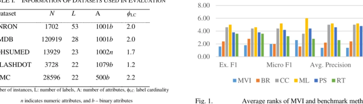
The summarized result in Fig. 1 shows that MVI has the best average rank for all measures except Macro F1. For this performance metric, the proposed method ranks second after BR. The more detailed result can be found in TABLE II, where the value of performance measures is supplied together with its per-dataset ranking in parenthesis.
For all 6 measures, MVI, BR and RT are the top 3 methods regarding their average ranks. MVI learns well on 3 datasets: small ENRON, SLASHDOT, and big IMDB. Especially, on SLASHDOT, the performance of MVI is far better than that of all other benchmark methods. BR do well on TMC and OHSUMED.
Overall, our proposed method performs well on all 6 mentioned measure. BR and RT achieve quite competitive results, meanwhile CC, PS have a big variation in performance. Clearly, the simplest method ML performs weakly.
The time cost of all the mentioned algorithms is depicted in TABLE III. MVI has a moderate average time cost (201.86 seconds), which is much smaller than that of BR (534.88 seconds), CC (542.58 seconds). In particular, the proposed
method is quicker than the two competitive methods BR and RT. Although MVI are slower than ML and PS, compared to these methods, MVI’s classification performance is much better.
VI. CONCLUSIONS
We have presented an online multi-label classification algorithm based on variational inference and random projection. Besides achieving superior performance over several well-known benchmark algorithms, MVI has a moderate time cost which can be further reduced by parallelization. As the proposed method is a flexible second-order generative framework which gives not just a point estimate but a distribution of solutions, our future work will be to investigate its application in other advanced tasks of multi-label learning such as cost-sensitive learning, imbalanced learning and adaptive learning.
ACKNOWLEDGMENT
Thi Thu Thuy Nguyen is supported by the Australian Government Research Training Program Scholarship to undertake this research. This project is partially supported by the Science and Technology Foundation of Guangdong Province Project No. 2017A050501002
REFERENCES
[1] F. Herrera, F. Charte, A.J. Rivera, and M.J. del Jesus, Multi-label classification, Springer, 2016.
[2] T.T.T. Nguyen, T.T. Nguyen, A.W.-C. Liew, and S. Wang, “Variational inference based Bayes online classifiers with concept drift adaptation”, vol. 81, pp. 280-293, 2018.
[3] J. Read, A. Bifet, G. Holmes, and P. Pfahringer, “Scalable and efficient multi-label classification for evolving data streams”, Machine Learning, vol. 88, pp. 243–272, 2012.
[4] M.-L. Zhang, and Z.-H. Zhou, “A review on Multi-label learning algorithms”, IEEE Transactions on Knowledge and Data Engineering, vol. 26(8), pp. 1819-1837, 2014.
[5] X.Z. Fern and C.E. Brodley, “Random projection for high dimensional data clustering: A cluster ensemble approach,” in ICML, 2003. [6] T.T.T. Nguyen, A.W.-C. Liew, T.T. Nguyen, S. Wang, “A novel
Bayesian framework for online imbalanced learning”, in DICTA, 2017. [7] M.R. Boutell, J. Luo, X. Shen, and C. M. Brown, “Learning multi-label scene classification”, Pattern Recognition, vol. 37(9), pp. 1757– 1771,2004.
[8] J. Read, B. Pfahringer, G. Holmes, and E. Frank, “Classifier chains for multi-label classification”, Machine Learning 85(3), pp. 333–359, 2011.
[9] J. Read, B. Pfahringer, and G. Holmes, “Multi-label classification using ensembles of pruned sets”, in ICDM, 2008.
[10] M.-L. Zhang, and Z.-H. Zhou, “ML-kNN: A lazy learning approach to multi-label learning”, Pattern Recognition, vol 40(7), pp. 2038–2048, 2007.
[11] A. Elisseeff, and J. Weston, “A kernel method for multi-labelled classification”, in NIPS, 2002.
[12] C. Vens, J. Struyf, L. Schietgat, S. Dˇzeroski, and H. Blockeel, “Decision trees for hierarchical multi-label classification”, Machine Learning, vol. 73(2), pp. 185–214, 2008.
[13] J. Read, P. Reutemann, B. Pfahringer, and G. Holmes, “MEKA: A Multi-label/Multi-target Extension to WEKA”, Journal of Machine Learning Research, vol. 17(21), pp. 1−5, 2016.
[14] P. Domingos, and G. Hulten, “Mining high-speed data streams”, in SIGKDD, 2000.
[15] T.T. Nguyen, T.T.T. Nguyen, X.C. Pham, and A.W.C. Liew, “A novel combining classifier method based on Variational Inference”, Pattern Recognition, vol. 49, pp. 198-212, 2016.
[16] R. Avogadri, and G. Valentini, “Fuzzy ensemble clustering based on random projections for DNA microarray data analysis”, Artificial Intelligence in Medicine, vol. 45: 173-183, 2009.
[17] S. Dasgupta, and A. Gupta, “An elementary proof of a theorem of Johnson and Lindenstrauss”, Random Structures & Algorithms, vol. 22(1), pp. 60–65, 2003.
[18] W. Johnson, and J. Lindenstrauss, “Extensions of Lipschitz mapping into Hilbert space”, in Conference in modern analysis and probability, 1984.
[19] E. Bingham, and H. Mannila, “Random projection in dimensionality reduction: applications to image and text data”, in KDD, 2001. [20] T.T. Nguyen, T.T.T. Nguyen, X.C. Pham, A.W.-C. Liew, and J.C.
Bezdek, “An ensemble-based online learning algorithm for streaming data”, arXiv:1704.07938, 2017.
[21] X.Z. Fern, C.E. Brodley, “Random Projection for High Dimensional Data Clustering: A Cluster Ensemble Approach”, in ICML, 2003. [22] J. Gama, Knowledge discovery from data streams, 1st ed.: Chapman &
TABLE I. INFORMATION OF DATASETS USED IN EVALUATION Dataset N L A ϕLC ENRON 1702 53 1001b 2.0 IMDB 120919 28 1001b 2.0 OHSUMED 13929 23 1002n 1.7 SLASHDOT 3728 22 1079b 1.2 TMC 28596 22 500b 2.2
N: number of instances, L: number of labels, A: number of attributes, ϕLC: label cardinality
n indicates numeric attributes, and b – binary attributes Fig. 1. Average ranks of MVI and benchmark methods
TABLE II. PERFORMANCE MEASURES OF MVIAND BENCHMARK ALGORITHMS
ENRON IMDB OHSUMED SLASHDOT TMC Avg. Rank↓
(a) Ex. F1↑ MVI 0.4790 (1) 0.3132 (1) 0.2835 (3) 0.3552 (1) 0.6153 (2) 1.60 BR 0.4566 (2) 0.2332 (5) 0.3225 (2) 0.1652 (2) 0.6256 (1) 2.40 CC 0.3933 (4) 0.0915 (6) 0.2425 (4) 0.0278 (6) 0.6146 (3) 4.60 ML 0.2021 (6) 0.2483 (3) 0.1432 (6) 0.1484 (4) 0.2166 (6) 5.00 PS 0.2778 (5) 0.2420 (4) 0.3316 (1) 0.1438 (5) 0.5696 (4) 3.80 RT 0.4422 (3) 0.3095 (2) 0.1986 (5) 0.1628 (3) 0.5378 (5) 3.60 (b) Ex.Accuracy↑ MVI 0.3625 (1) 0.2342 (1) 0.2175 (3) 0.3218 (1) 0.5048 (3) 1.80 BR 0.3417 (2) 0.1710 (5) 0.2579 (2) 0.1451 (4) 0.5199 (1) 2.80 CC 0.2979 (4) 0.0710 (6) 0.2110 (4) 0.0263 (6) 0.5185 (2) 4.40 ML 0.1680 (6) 0.2081 (3) 0.1270 (6) 0.1458 (2) 0.1786 (6) 4.60 PS 0.2246 (5) 0.2032 (4) 0.2902 (1) 0.1407 (5) 0.4804 (4) 3.80 RT 0.3239 (3) 0.2272 (2) 0.1548 (5) 0.1452 (3) 0.4220 (5) 3.60 (c) Micro F1↑ MVI 0.4773 (1) 0.3240 (2) 0.3196 (4) 0.3774 (1) 0.6372 (2) 2.00 BR 0.4443 (3) 0.2580 (3) 0.3770 (1) 0.1811 (2) 0.6384 (1) 2.00 CC 0.3990 (4) 0.1263 (6) 0.3206 (3) 0.0509 (6) 0.6346 (3) 4.40 ML 0.1427 (6) 0.2379 (4) 0.1374 (6) 0.1411 (4) 0.1988 (6) 5.20 PS 0.2547 (5) 0.2309 (5) 0.3297 (2) 0.1379 (5) 0.5731 (4) 4.20 RT 0.4723 (2) 0.3267 (1) 0.2251 (5) 0.1611 (3) 0.5340 (5) 3.20 (d) Macro F1↑ MVI 0.1048 (1) 0.0551 (3) 0.0914 (4) 0.1652 (1) 0.3494 (4) 2.60 BR 0.0650 (2) 0.0859 (1) 0.2980 (1) 0.0840 (2) 0.4612 (2) 1.60 CC 0.0440 (5) 0.0452 (4) 0.2589 (2) 0.0468 (4) 0.4456 (3) 3.60 ML 0.0090 (6) 0.0245 (6) 0.0135 (6) 0.0133 (6) 0.0232 (6) 6.00 PS 0.0464 (4) 0.0277 (5) 0.1478 (3) 0.0397 (5) 0.1905 (5) 4.40 RT 0.0474 (3) 0.0561 (2) 0.0345 (5) 0.0562 (3) 0.5173 (1) 2.80
(e) Avg. Precision↑
MVI 0.5656 (1) 0.4695 (2) 0.4643 (2) 0.5281 (1) 0.7669 (1) 1.40 BR 0.5265 (3) 0.4153 (3) 0.5170 (1) 0.3763 (2) 0.7468 (2) 2.20 CC 0.3709 (4) 0.1841 (6) 0.3684 (5) 0.2547 (6) 0.6423 (4) 5.00 ML 0.2409 (6) 0.3003 (4) 0.2700 (6) 0.2986 (4) 0.2860 (6) 5.20 PS 0.2934 (5) 0.2959 (5) 0.4220 (3) 0.2919 (5) 0.5953 (5) 4.60 RT 0.5438 (2) 0.4754 (1) 0.3809 (4) 0.3442 (3) 0.7122 (3) 2.60 (f) Ranking Loss↓ MVI 0.1694 (2) 0.1777 (2) 0.2083 (1) 0.1779 (1) 0.0660 (1) 1.40 BR 0.1922 (3) 0.2185 (3) 0.2135 (2) 0.2346 (2) 0.1040 (2) 2.40 CC 0.3803 (4) 0.4934 (6) 0.3652 (5) 0.4048 (6) 0.2254 (4) 5.00 ML 0.5095 (6) 0.4514 (4) 0.4376 (6) 0.3705 (4) 0.5848 (6) 5.20 PS 0.4594 (5) 0.4532 (5) 0.3350 (4) 0.3757 (5) 0.2826 (5) 4.80 RT 0.1196 (1) 0.1719 (1) 0.2566 (3) 0.2655 (3) 0.1118 (3) 2.20
TABLE III. TIME COST↓(IN SECONDS)OF MVIAND BENCHMARK ALGORITHMS ENRON IMDB OHSUMED SLASHDOT TMC Average MVI 24.69 765.91 73.08 16.69 128.94 201.86 BR 58.33 2246.40 184.11 50.54 135.01 534.88 CC 58.58 2257.23 193.73 48.43 154.94 542.58 ML 0.19 1.85 0.36 0.15 0.52 0.62 PS 2.68 57.40 28.64 8.69 15.78 22.64 RT 68.82 1184.84 84.08 26.74 86.32 290.16 0.00 2.00 4.00 6.00 8.00
Ex. F1 Micro F1 Avg. Precision