Studienabschlussarbeiten
Fakultät für Mathematik, Informatik
und Statistik
Le, Minh-Anh:
Anomaly Detection using Machine Learning Methods
Implementation and Benchmark Analysis of Selected
Methods and Tuning Criteria
Masterarbeit, Wintersemester 2018
Fakultät für Mathematik, Informatik und Statistik
Ludwig-Maximilians-University
Master Thesis
Anomaly Detection using Machine Learning Methods
Implementation and Benchmark Analysis of Selected Methods and Tuning CriteriaAuthor: Minh-Anh Le
Supervisor: Prof. Dr. Bernd Bischl
Laura Beggel
Contents
1 Introduction 1
2 Anomaly Detection 2
2.1 Definition of Anomalies . . . 2
2.1.1 Nature of Input Data . . . 3
2.1.2 Types of Anomaly . . . 3
2.1.3 Availability of Labels . . . 4
2.2 Application of Anomaly Detection . . . 5
2.3 Challenges . . . 6
3 Evaluation 6 3.1 Supervised Performance Measurement . . . 7
3.2 Unsupervised Performance Measurement: Area under the Mass-Volume Curve (AUMVC) . . . 9
3.2.1 Mass-Volume Curve (MV curve) . . . 11
3.2.2 Area under the Mass Volume Curve (AUMVC) . . . 16
3.2.2.1 Tuning Hyper parameters with AUMVC . . . 17
3.2.2.2 Computing the Volume in AUMVC . . . 17
3.2.2.3 AUMVC on High-Dimensional Data (AU M V Chd) . 17 3.2.2.4 Choosing the IntervalI forAU M V C and AU M V Chd 19 4 Unsupervised Anomaly Detection Methods 20 4.1 Support Vector Machine (SVM) . . . 20
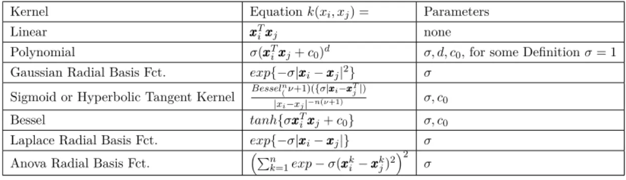
4.1.1 Kernels and The Kernel-trick . . . 24
4.1.2 Support Vector Machines for Anomaly Detection . . . 25
4.1.3 Tuning . . . 27
4.2 Local Outlier Factor (LOF) . . . 28
4.2.1 Tuning . . . 31
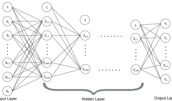
4.3 Neural Network (NN) . . . 31
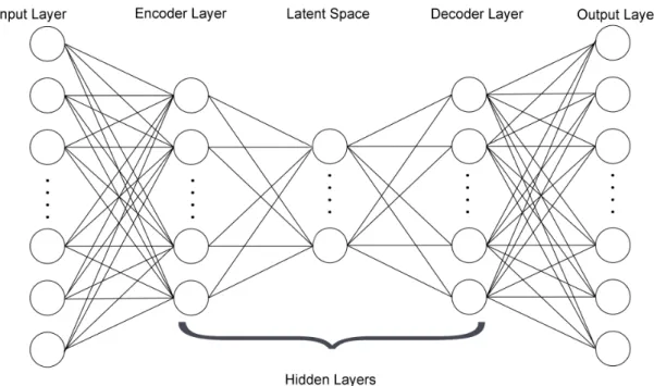
4.3.1 Neural Network for Anomaly Detection: Deep Autoencoders 35 5 Resampling Strategies for One-Class Classification 36 6 Converting Anomaly Score Outputs into Probabilistic Outputs 37 6.1 Probabilistic Output for Supervised Classification . . . 39
6.2 Probabilistic Output for Unsupervised Anomaly Detection . . . 40
7 Open Source R Package: mlR 43 7.1 What ismlR . . . 43
7.2 General Structure of mlR. . . 45
7.3 Anomaly Detection in mlR . . . 46
7.3.1 New and modified Functions for Anomaly Detection in mlR . 47 7.3.2 Package e1071 . . . 48
7.3.4 Package DMwR . . . 48
7.3.5 Package dbscan . . . 48
7.3.6 Package h2o.deeplearning . . . 49
7.4 Application of Anomaly Detection in mlR . . . 49
8 Benchmark Setup 49 8.1 Data Sets . . . 49
8.1.1 Synthetic Data Sets . . . 50
8.1.2 Open Source Data Sets . . . 50
8.2 Method and AUMVC(hd) Settings . . . 51
9 Benchmark Results 52 9.1 Performance and Runtime Analysis of AUMVC(hd) . . . 53
9.1.1 Runtime Analysis . . . 53
9.1.2 Fluctuation of the AUMVC(hd) . . . 58
9.1.3 AUMVC(hd) Performance w.r.t. Number of Monte-Carlo Sam-ples . . . 60
9.1.4 AUMVC(hd) Performance w.r.t. Number of Splits of the Al-pha Interval . . . 64
9.1.5 AUMVChd Performance w.r.t. to Number of Internal Sub-samples . . . 66
9.2 Performance Analysis under Different Experiments Setups . . . 68
9.2.1 Tuning with Tuning Measurement AUMVC and AUMVChd . 71 9.2.1.1 AUMVC on Low Dimensional Data . . . 71
9.2.1.2 AUMVChd on High Dimensional Data . . . 73
9.2.2 Training and Tuning with Cross-Validation vs. One-Class Cross-Validation for OC-SVM . . . 75
9.2.2.1 AUMVC on Low Dimensional Data . . . 75
9.2.2.2 AUMVChd on High Dimensional Data . . . 77
9.2.3 Comparison of Methods OC-SVM and LOF . . . 78
9.2.3.1 AUMVC on Low Dimensional Data . . . 79
9.2.3.2 AUMVChd on High Dimensional Data . . . 80
9.2.4 Analysis of the Autoencoder . . . 81
9.2.4.1 AUMVC on Low Dimensional Data . . . 82
9.2.4.2 AUMVChd on High Dimensional Data . . . 85
10 Summary 87
Appendices 94
A Additional Measurement for Imbalanced Class Sizes 94
1 Introduction
Outliers or anomalies are a common occurrence in data. They can for instance re-sult from defected measurement devices, wrongly transferred data, human error, fraud, change in population or other reasons. In the past, many methods were developed to address this issue, such as Z-score analysis, linear regression models, probabilistic and statistical modeling. But in times of increasing computational power, increasing amount of produced data, new possibilities to store data and advanced algorithms, many con-ventional statistical methods aren’t adequate anymore. As a result, machine learning methods become increasingly important.
Detecting and differentiating anomalies from normal data is a classification problem. However, the differences of binary classification and anomaly detection are also the no-table challenges, namely the lack of labels and highly unbalanced class data. In some cases, only data from one class are available. Thus, anomaly detection algorithms which can train on data containing only one class are also called one-class classification. The learning problem is then described as semi-supervised. If there is no information about the data set available at all, the learning problem is then described as unsupervised. The first aim of this work is to analyse three different machine learning methods to detect anomalies for semi-supervised and unsupervised settings, which are the one-class support vector machine (OC-SVM), local outlier factor (LOF) and autoencoder (AE). Moreover, performance measurements to tune hyper parameter sets and the evaluation of the used methords are of special interest. With the lack of labels, there are no possi-bilities to use performance measurement of classic binary classification. As it is essential to draw conclusions about the quality of used methods or it chosen hyper parameter sets an unsupervised performance measurement is investigated in this work.
The second aim of this work is to implement the anomaly detection class into the already established mlRpackage in Rand make it available for other users.
This work starts with a general definition of the term "Anomalies" in Section 2.1 and how the application of anomaly detection methods depends on the nature of input data in Sections 2.1.1. Section 2.2 gives two short examples of real-life anomaly detection cases. Major challenges of anomaly detection are covered in Section 2.3. Since choosing an ap-propriate evaluation measure is one of the main challenges, Section 3.1 covers supervised measurements and Section 3.2 a new defined unsupervised measurement "Area under the Mass Volume Curve (AUMVC)". The measurement can be used on any anomaly de-tection methods such as the one-class SVM (Section 4.1), local outlier factor (LOF) (Section 4.2) or autoencoders (AE) (Section 4.3). To apply tuning on those methods, additional resampling strategies are introduced in Section 5. Following the algorithm in Section 6, the score value outputs of the methods are converted into probabilities to embed the methods into mlR and to guarantee some other advantages listed in Sec-tion 6. SecSec-tion 7 gives a brief overview of the mlR package in R, what has been done to implement the anomaly detection class into mlR as well as how to use the newly implemented class. Finally, Section 8 explains the used data sets and settings for the following benchmark analysis in Section 9. The results section is divided into two parts:
the first is about investigating the AUMVC and its settings (Section 9.2), the second about using AUMVC(hd) with the previously introduced anomaly detection methods (Section 9.2.1). And lastly, Section 10 gives a summary of the results of this work. The Appendix contains additional measurements for unbalanced class sizes (A), tables, and figures to provide more details of the results (B).
2 Anomaly Detection
Throughout the years several anomaly detection methods have been developed. The typical anomaly detection methods build models of normal data and detect deviations from the normal model in observed data [Eskin et al., 2002, p. 79]. However, to formulate the specific anomaly detection problem, the following aspects need to be taken into consideration: the nature of the input data (Section 2.1.1), type of anomalies (Section 2.1.2), availability of labels (Section 2.1.3) and constraints and requirements from the application domain [Chandola et al., 2009, p. 6]. This section starts with the definition of anomalies in Subsection 2.1, before focusing on the above mentioned aspects.
2.1 Definition of Anomalies
According to the Oxford English Dictionary, ananomalyis "something that deviates from what is standard, normal, or expected". In the data context, anomalies are observations, which deviate from the majority of the data [Amer et al., 2013, p. 1]. Depending on the application domain, anomalies are also referred to as outliers, discordant observations, exceptions, aberrations, surprises, peculiarities, contaminants [Chandola et al., 2009, p. 1], novelties, noise or deviations [Dau et al., 2014, p. 2].
Some popular definitions are
• "An outlying observation, or outlier, is one that appears to deviate markedly from other members of the sample in which it occurs." [Grubbs, 1969]
• "An observation (or subset of observations) which appears to be inconsistent with the remainder of that set of data." [Hodge and Austin, 2004, p. 2]
• "An outlier is an observation which deviates so much from other observations as to arouse suspicions that it was generated by a different mechanism." [Hawkins, 1980]
• "Anomaly detection refers to the problem of finding patterns in data that do not conform to expected behaviour." [Chandola et al., 2009, p. 1]
There are two ways of handling anomalies, either delete or correct them, for example to yield statistically significant increase in accuracy [Smith and Martinez, 2011, p. 1] or translate them into significant actionable information [Chandola et al., 2009, p. 1]. Anomalies caused by measurement errors, for instance, are a good example of anomalies that should be deleted. In contrast to this, anomalous traffic patterns in a computer
network that could be interpreted as a hacker attack, are a good example of anomalies that should be detected to prevent it [Kumar, 2005].
In both cases, methods are needed to find these anomalies. Methods that find, delete, modify or ignore anomalies are often referred to as noise removal and noise accommo-dation [Hodge and Austin, 2004, p. 4]. Whereas methods that find anomalies toextract relevant informationare referred to asanomaly detection. Since both categories of meth-ods are related, the above mentioned definitions of anomaly detection are suitable for both types. The aim of anomaly detection in machine learning is to build a model that can differentiate anomalies from the remaining normal data [Dau et al., 2014, p. 2]. In this work, we will focus on anomaly detection with machine learning techniques in order to retrieve interesting information from the database.
2.1.1 Nature of Input Data
The applicability of anomaly detection methods depends on the nature of the input data, i.e., the characteristics of the input data. Input data usually contains a collection of instances which can be described as univariate, multivariate, binary, categorical or continuous [Chandola et al., 2009, p. 6]. Those attributes affect the range of methods to choose from. Moreover, the instances can have a relationship with each other, e.g., sequence data such as time series, spatial data or graph data. If no relationship among the data instances is assumed, one is dealing with record data or so-called point data. In this work we will assume to have point data with only continuous features. For these characteristics the OC-SVM (Section 4.1), LOF (Section 4.2) and AE (Section 4.3) are applicable.
2.1.2 Types of Anomaly
Before applying an anomaly detection method, it is also crucial to know which type of anomaly is present [Chandola et al., 2009, p. 8].
We can make a distinction based on whether the data containspoint anomalies, collec-tive anomalies or contextual anomalyies.
Point Anomaly is the simplest type of anomaly. Point anomaly is an individual data instance, which is anomalous with respect to the rest of the data [Chandola et al., 2009, p. 7]. A simple real life example is credit card fraud when only the amount spent by a person is analyzed: a transaction where the amount spent is much higher than the average amount spent is likely to be a point anomaly. But in the context of time, this kind of a transaction during Christmas instead of a summer month might be normal for that person. In the summer month, this kind of transaction would be referred to as contextual anomaly. Therefore, the contextual anomaly can be determined by con-sidering behavioural attributes, e.g. amount spent within contextual attributes, such as time. [Chandola et al., 2009, p. 8]. Another type is collective anomaly, which only occurs in data sets with related instances. The single data points in a collective anomaly
may not be considered as anomalies by themselves, but the occurrence of these single points together indicates an anomaly [Bontemps et al., 2016, p. 2]. In the example of credit card fraud, a transaction for which the amount spent is in the normal range, is considered as normal. Now, if this amount of transaction happens every hour of a day, the occurrence together as a collection is anomalous.
2.1.3 Availability of Labels
Besides the nature of input data and anomaly type, the availability of labels is also essen-tial when it comes to selecting the anomaly detection method. However, the availability of labels is one of the biggest challenges [Dau et al., 2014, p. 1]. Collecting labels is very expensive and requires a lot of effort, as it is often done manually by human experts [Chandola et al., 2009, p. 10]. This fact leads to three fundamental approaches to the problem of anomaly detection: supervised, semi-supervised and unsupervised anomaly detection.
Supervised Anomaly Detection The ideal situation would be to have a training data set with labels for anomalies and normal data. In this case, it is a classification problem [Hodge and Austin, 2004, p. 5], where the classifier learns the classification model. However, this approach is limited to what the model has seen before or what is known as anomalies, thus it requires at least enough data to cover the entire distribution of each class in order to generalize a classifier [Hodge and Austin, 2004, p. 6]. This is usually not the use case as labeled anomalous data is expensive to get [Hodge and Austin, 2004, p. 7] or the share of anomaly data is too small to derive a generalized distribution. A summary on how to handle classification and imbalanced classification problems can be found in the online tutorial of mlR (see [mlr]).
Semi-supervised Anomaly Detection In the case that the data is only labeled for the normal class, the problem can be categorized as a one-class learning problem for which semi-supervised anomaly detection techniques are needed. The main idea is to train a model for the class of normal behaviours, which is then used in the test data to identify anomalous behaviour [Chandola et al., 2009, p. 11], [Amer et al., 2013, p. 1]. This approach is analogous to the semi-supervised recognition of detection, where the model learns only the normal class and derives a boundary of normality [Hodge and Austin, 2004, p. 6]. For this approach, the methods don’t require anomalous data for training but enough labeled normal data to be able to derive a generalized distribution [Hodge and Austin, 2004, p. 6]. The semi-supervised anomaly detection method is the most used one, just take for example production machines, cars or any machines, they usually run as expected and the produced data can be labeled as normal data. It is hard to simulate a situation which is not normal, and even if it would be possible to simulate this situation, there is no possibility to know if all potential situations of anomalies are
covered.
The methods one-class SVM and autoencoder are semi-supervised detection methods (see Section 4.1 and Section 4.3) and can be applied on the one-class learning problem.
Unsupervised Anomaly Detection Another common and challenging situation is to have no labeled data at all. Basically, the challenge is the non-existence of prior knowledge about the data, e.g. the question which oberservations are anomalous or what share of the data is anomalous etc. This situation is referred to as unsupervised anomaly detection [Hodge and Austin, 2004, p. 4]. To apply unsupervised anomaly detection techniques, no separation of training and testing phase is needed. Additionally [Amer et al., 2013, p. 1], one needs to make the implicit assumption that normal instances are far more frequent than anomalies [Chandola et al., 2009, p. 11] and that anomalies can be separated from the normal data [Hodge and Austin, 2004, p. 4]. The underlying concept is to model a static distribution and mark remote points as potential anomalies. For the unsupervised setting, a popular method is the local outlier factor (LOF), which is further described in Section 4.2.
2.2 Application of Anomaly Detection
Anomaly detection plays an important role in many areas such as intrusion detection, fraud detection, medical anomaly detection, industrial damage detection or anomaly de-tection in text [Chandola et al., 2009, p. 11].
An example of a medical anomaly detection problem is the mammography data set (Section 8.1). Mammography is one of the most effective methods for screening breast cancer. Physicians interpret the screening and decide whether a biopsy to extract sam-ple cells or tissue is necessary to confirm the presence of breast cancer. However, 70% biopsies have a benign outcome and are therefore unnecessary [Elter et al., 2007]. In order to reduce those unnecessary biopsies, the learning algorithm should help to predict the type of tumor based on mammography screens. To train the model a data set with the attributes age, shape, margin and density can be used to predict if the mammography screen is likely to show a benign (normal) or malignant (anomaly) tu-mor. Most of the labeled data belongs to healthy patients, thus classification for highly unbalanced class data or semi-supervised anomaly detection methods can be used to train the model.
Another example is intrusion detection that refers to the detection of malicious activity in a computer-related system [Chandola et al., 2009, p. 12]. Especially when computer systems store sensible data (such as patient data, government data, customer data, etc.), the security for protecting the system against intrusion or so-called hacker attacks should be very high. One of the challenges of this problem is the constant modification of these attacks. Over time attackers will learn how to outsmart the detection system, and over time the detection system is improved to shield again newly evolved attacks. Since the only sure knowledge about the system is how the normal status look likes, semi-supervised or unsemi-supervised anomaly detection methods should be preferred [Chandola et al., 2009, p. 12].
2.3 Challenges
First evidence for challenges in anomaly detection is described in the previous section when dicussing the availability of labels. The availability of labels does not only de-termine the method of choice, but also the limits of the the possibilities to tune the chosen model or to evaluate if the chosen model could actually detect anomalies in new, unlabeled data. Thus training, but also validation of the model is one of the major challenges in anomaly detection [Chandola et al., 2009, p. 3].
In addition, normal data as well as anomalies evolve over time in many areas, thus cur-rent anomalies but also normal data might not be representative for future observations. Furthermore, if anomalies occurred due to intervention of, e.g., hackers, these anomalies would appear to be similar to normal data. Hence it is more difficult for the model to distinguish between anomalies and normal oberservations or to define a normal train-ing set for semi-supervised anomaly detection methods. The definition of the normal data set is another challenge, as covering all possible normal behaviour is very difficult. Additionally, anomalies in different domains might differ in their behaviour. In some domains, slight deviation from the normal behaviour is already tagged as anomalous whereas in others the same anomalies might be tagged as normal. Similar to judging if noise in the data are anomalies or normal. [Chandola et al., 2009, p. 3]
Due to those challenges, anomaly detection is a wide and underresearched area. Many anomaly detection methods and research papers are solving one specific problem for a specific characteristic of input data and domain. Those methods are developed from dis-ciplines such as statistics, machine learning, data mining and others. [Chandola et al., 2009, p. 3]
In the following, this work will focus on semi-supervised and unsupervised machine learn-ing methods applied to data containlearn-ing point anomalies, while not taklearn-ing into account the specific domain where the data comes from.
3 Evaluation
Evaluation criteria, also called performance measurements, help the user to choose an optimal method for a data set and the problem at hand. Therefore the evaluation criteria should be chosen at the beginning and used as an optimization criteron. The choice of performance measurement depends on the type of output of the anomaly detection method, which can be either scores or labels and the availability of true labels. If true labels are given the user should use supervised performance measurements (Subsection 3.1), otherwise unsupervised performance measurements (Subsection 3.2).
For methods that return scores, the analyst needs to define an optimal threshold to determine the anomalies, which can be done domain specific or model specific [Chandola et al., 2009, p.11]. For returned labels the analyst can indirectly control the threshold by controlling parameters within each method (e.g. controlling the ‹ variable in the OC-SVM method) [Chandola et al., 2009, p.11]. In order to find the optimal controlling parameter or threshold the user can again tune the model with an appropriate evaluation
criterion. As anomaly detection methods classify the observation in two classes (normal and anomaly), if labels are available for testing, most of the known binary classification performance measurements as well as a view anomaly detection specific performance measurements can be used (Section 3.1). There are almost no performance measurements available yet for data without labels, but one recently developed method is the Area under the Mass Volume curve (AUMVC), which is introduced in Section 3.2 and further analyzed in (Section 8).
3.1 Supervised Performance Measurement
Although unsupervised anomaly detection deals with unlabeled data, most anomaly de-tection papers use labels to evaluate their algorithms. In more detail, they train the model on unsupervised data but evaluate the performance of the algorithm using true labels. By doing so, a comparison over different anomaly detection algorithms is possible (e.g. Hodge and Austin [2004] or Goldstein and Uchida [2016]). But in practice, the true labels are usually not available. Section 3.2 deals with this situation.
In this section some supervised performance measurements, which are commonly used for anomaly detection, are introduced. Since we assume labeled data for evaluation, most of them are performance measurements for binary classification, that are also suitable for data with imbalanced class sizes, such as AUC, F-Score, true positive rate and true negative rate (e.g. Campos et al. [2016]). Nevertheless, not all measurements derived from the confusion matrix are adequate for the specific case of anomaly detection. For instance, the accuracy measureACC defined as (T P +T N)/N (see definition in Figure 1) is not suitable for imbalanced classes. In anomaly detection we usually expect a max-imal share of 10% of anomalies, therefore the TP is comparatively small to the TN and the proportion between TP and TN is highly unbalanced. Thus, although in case the algorithm performs worse in detecting anomalies, its ACC can still yield a high value. For this reason, Campos et al. [2016, p.900] introduce additional performance measure-ments such as the weighted accuracy, top-p accuracy, precision at n, adjusted precision at n or average precision at n, which will be explained in more detail in Appendix A and are also implemented in mlR.
For the benchmark analysis, we only focus on the AUC as supervised performance mea-surement for anomaly detection.
Overview of some notations in this section:
• O: set of true anomalies or outliers in the data set • I: set of true normal observations
Confusion matrix In supervised classification, a confusion matrix is often used for evaluation, as it indicates whether the algorithm confuses two classes. An overview of the content of a confusion matrix and measures that can be derived from it are displayed in Figure 1.
Figure 1: A confusion matrix, partly taken out from Fawcett [2006, p.2]. The positive class is the anomaly class (P), the negative class the normal class (N).
Most of the measures in Figure 1 are commonly known and self-explanatory Fahrmeir et al. [2016], the rest is shortly described in the following:
• The F1 does not take the TN (=normal) class into account, which is favorable as the focus in anomaly detection is on detecting anomalies [Garcıa et al., 2009, p.1].F1 œ[0,1], where 1 is indicating best prediction.
• The G-mean is the geometric mean of TPR and PPV and is also considered as a measure suitable for imbalanced data [Kubat et al., 1997, p.2]. G-mean œ [0,1], where 1 indicates best prediction.
• Bac is also a performance measure for skewed class distributions [Garcıa et al., 2009, p.1], that compares the number of positives and negatives relative to their class sizes (TPR and TNR). Bac œ[0,1], where 1 indicates best prediction. • Thewacis a weightedbac. For weightsw= 0.5 thewacis thebac. Althoughbacis
already suitable for imbalanced data, the user can focus more on the detection of anomalies (positive class) than the detection of the normal class (negative class).
ROC and AUC The Receiver-Operating-Characteristic-Curve (ROC) is a graphical method to evaluate the performance of an algorithm. ROC plots the TPR against the FPR [Powers, 2011, p.4]. Algorithms yielding coordinates in the far top left corner, which means having a FPR of 0 and a TPR of 1, are the best classifiers (and vice versa for the worse classifiers). Algorithms that classify as good as random guessing will score along the diagonal, whereT P R=F P R[Powers, 2011, p.4]. Therefore, a classifier whose ROC curve is strictly above the ROC of another classifier is considered to perform better in terms of the ROC. Thus the ROC is a tool to compare different classifiers [Powers, 2011, p.4]. In cases where two ROC curves intersect, it is sometimes hard to determine which classifier performs better. In case the user wants to perform tuning with several different settings, a visual evaluation isn’t effective nor accurate enough. Instead of using the ROC curve we can summarize the ROC in one value, thearea under the curve
(AUC). The classifier that has a higher AUC value performs better. The ROC and AUC are insensitive to imbalanced data, as they consider TPR and FPR. As the AUC is one
of the most popular measures, which is widely used in other anomaly detection papers, we will use it as the benchmark measure for the experiments in Section 8.
3.2 Unsupervised Performance Measurement: Area under the Mass-Volume Curve (AUMVC)
One of the key challenges in unsupervised learning is to evaluate performance without having access to labels. Until today, there is no established way to measure performance in unsupervised learning. Most of the papers dealing with anomaly detection build the model on data pretending to don’t have labels, but evaluate on data with labels, as their objective is simply to compare different algorithms in a general manner, see for example Goldstein and Uchida [2016]. Research is beginning to develop measurements to ad-dress the problem of unsupervised performance measures. For example the algorithm in Thomas et al. [2016] and Goix [2016], both based on the theory of the Mass-Volume Curve (MV curve) for scoring functions from which they extract a scalar measurement value called the Area under the Mass-Volume curve. It can be applied on low dimen-sional data (AUMVC) with less than 8 features or high dimendimen-sional data (AUMVChd). The AUMVC is specifically developed for tuning in the unsupervised setting.
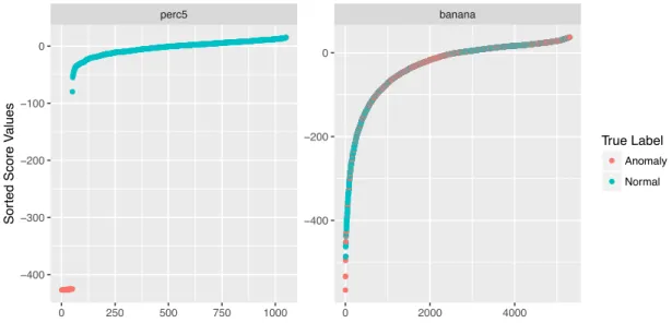
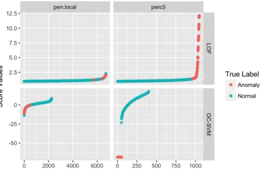
Figure 2 is a visualization of the problem of unsupervised learning of hyper parameter, it shows the sorted scores for the data sets 5perc and banana (see Section 2.1.3). In unsupervised learning, it is usually not possible to color the data points, (anomalies red and the normal observation blue). Imagine we would set a threshold based on this two graphics (without colors). For the left we would choose a threshold at ≠50 and if we have the labels, we would know that the chosen threshold is an appropriate one. For the right graphic we would choose a threshold around≠500. With labels, one can verify that there isn’t any appropriate threshold, as the anomaly detection algorithm was already failing to calculate a correct scoring function to map the data. But as labels are not available, we wouldn’t know how appropriate the threshold is.
● ● ● ●●●●●●●●●●●●●●●●●●●●●●●●●●●●●●●●●●●●●●●●●●●●●●● ● ● ● ● ●●●●●●●●●●●●●●●●●●●●●●●●●●●●●●●●●●●●●●●●●●●●●●●●●●●●●●●●●●●●●●●●●●●●●●●●●●●●●●●●●●●●●●●●●●●●●●●●●●●●●●●●●●●●●●●●●●●●●●●●●●●●●●●●●●●●●●●●●●●●●●●●●●●●●●●●●●●●●●●●●●●●●●●●●●●●●●●●●●●●●●●●●●●●●●●●●●●●●●●●●●●●●●●●●●●●●●●●●●●●●●●●●●●●●●●●●●●●●●●●●●●●●●●●●●●●●●●●●●●●●●●●●●●●●●●●●●●●●●●●●●●●●●●●●●●●●●●●●●●●●●●●●●●●●●●●●●●●●●●●●●●●●●●●●●●●●●●●●●●●●●●●●●●●●●●●●●●●●●●●●●●●●●●●●●●●●●●●●●●●●●●●●●●●●●●●●●●●●●●●●●●●●●●●●●●●●●●●●●●●●●●●●●●●●●●●●●●●●●●●●●●●●●●●●●●●●●●●●●●●●●●●●●●●●●●●●●●●●●●●●●●●●●●●●●●●●●●●●●●●●●●●●●●●●●●●●●●●●●●●●●●●●●●●●●●●●●●●●●●●●●●●●●●●●●●●●●●●●●●●●●●●●●●●●●●●●●●●●●●●●●●●●●●●●●●●●●●●●●●●●●●●●●●●●●●●●●●●●●●●●●●●●●●●●●●●●●●●●●●●●●●●●●●●●●●●●●●●●●●●●●●●●●●●●●●●●●●●●●●●●●●●●●●●●●●●●●●●●●●●●●●●●●●●●●●●●●●●●●●●●●●●●●●●●●●●●●●●●●●●●●●●●●●●●●●●●●●●●●●●●●●●●●●●●●●●●●●●●●●●●●●●●●●●●●●●●●●●●●●●●●●●●●●●●●●●●●●●●●●●●●●●●●●●●●●●●●●●●●●●●●●●●●●●●●●●●●●●●●●●●●●●●●●●●●●●●●●●●●●●●●●●●●●●●●●●●●●●●●●●●●●●●●●●●●●●●●●●●●●●●●●●●●●●●●●●●●●●●●●●●●●●●●●●●●●●●●●●●●●●●●●●●●●●●●●●●●●●●●●●●●●●●●●●●●●●●●●● ● ● ● ● ● ● ● ● ● ● ● ● ● ● ● ● ● ● ● ● ● ●●●●●●●●●●●●●●●●●●●●●●●●●●●●●●● ● ● ● ● ● ● ● ● ● ● ● ● ● ● ● ● ● ● ● ● ●●●●●●●●●●●●●●●●●●●●●●●●●●●●●●●●●●●●●●●●●●●●●●●●●●●●●●●●●●●●●●●●●●●●●●●●●●●●●●●●●●●●●●●●●●●●●●●●●●●●●●●●●●●●●●●●●●●●●●●●●●●●●●●●●●●●●●●●●●●●●●●●●●●●●●●●●●●●●●●●●●●●●●●●●●●●●●●●●●●●●●●●●●●●●●●●●●●●●●●●●●●●●●●●●●●●●●●●●●●●●●●●●●●●●●●●●●●●●●●●●●●●●●●●●●●●●●●●●●●●●●●●●●●●●●●●●●●●●●●●●●●●●●●●●●●●●●●●●●●●●●●●●●●●●●●●●●●●●●●●●●●●●●●●●●●●●●●●●●●●●●●●●●●●●●●●●●●●●●●●●●●●●●●●●●●●●●●●●●●●●●●●●●●●●●●●●●●●●●●●●●●●●●●●●●●●●●●●●●●●●●●●●●●●●●●●●●●●●●●●●●●●●●●●●●●●●●●●●●●●●●●●●●●●●●●●●●●●●●●●●●●●●●●●●●●●●●●●●●●●●●●●●●●●●●●●●●●●●●●●●●●●●●●●●●●●●●●●●●●●●●●●●●●●●●●●●●●●●●●●●●●●●●●●●●●●●●●●●●●●●●●●●●●●●●●●●●●●●●●●●●●●●●●●●●●●●●●●●●●●●●●●●●●●●●●●●●●●●●●●●●●●●●●●●●●●●●●●●●●●●●●●●●●●●●●●●●●●●●●●●●●●●●●●●●●●●●●●●●●●●●●●●●●●●●●●●●●●●●●●●●●●●●●●●●●●●●●●●●●●●●●●●●●●●●●●●●●●●●●●●●●●●●●●●●●●●●●●●●●●●●●●●●●●●●●●●●●●●●●●●●●●●●●●●●●●●●●●●●●●●●●●●●●●●●●●●●●●●●●●●●●●●●●●●●●●●●●●●●●●●●●●●●●●●●●●●●●●●●●●●●●●●●●●●●●●●●●●●●●●●●●●●●●●●●●●●●●●●●●●●●●●●●●●●●●●●●●●●●●●●●●●●●●●●●●●●●●●●●●●●●●●●●●●●●●●●●●●●●●●●●●●●●●●●●●●●●●●●●●●●●●●●●●●●●●●●●●●●●●●●●●●●●●●●●●●●●●●●●●●●●●●●●●●●●●●●●●●●●●●●●●●●●●●●●●●●●●●●●●●●●●●●●●●●●●●●●●●●●●●●●●●●●●●●●●●●●●●●●●●●●●●●●●●●●●●●●●●●●●●●●●●●●●●●●●●●●●●●●●●●●●●●●●●●●●●●●●●●●●●●●●●●●●●●●●●●●●●●●●●●●●●●●●●●●●●●●●●●●●●●●●●●●●●●●●●●●●●●●●●●●●●●●●●●●●●●●●●●●●●●●●●●●●●●●●●●●●●●●●●●●●●●●●●●●●●●●●●●●●●●●●●●●●●●●●●●●●●●●●●●●●●●●●●●●●●●●●●●●●●●●●●●●●●●●●●●●●●●●●●●●●●●●●●●●●●●●●●●●●●●●●●●●●●●●●●●●●●●●●●●●●●●●●●●●●●●●●●●●●●●●●●●●●●●●●●●●●●●●●●●●●●●●●●●●●●●●●●●●●●●●●●●●●●●●●●●●●●●●●●●●●●●●●●●●●●●●●●●●●●●●●●●●●●●●●●●●●●●●●●●●●●●●●●●●●●●●●●●●●●●●●●●●●●●●●●●●●●●●●●●●●●●●●●●●●●●●●●●●●●●●●●●●●●●●●●●●●●●●●●●●●●●●●●●●●●●●●●●●●●●●●●●●●●●●●●●●●●●●●●●●●●●●●●●●●●●●●●●●●●●●●●●●●●●●●●●●●●●●●●●●●●●●●●●●●●●●●●●●●●●●●●●●●●●●●●●●●●●●●●●●●●●●●●●●●●●●●●●●●●●●●●●●●●●●●●●●●●●●●●●●●●●●●●●●●●●●●●●●●●●●●●●●●●●●●●●●●●●●●●●●●●●●●●●●●●●●●●●●●●●●●●●●●●●●●●●●●●●●●●●●●●●●●●●●●●●●●●●●●●●●●●●●●●●●●●●●●●●●●●●●●●●●●●●●●●●●●●●●●●●●●●●●●●●●●●●●●●●●●●●●●●●●●●●●●●●●●●●●●●●●●●●●●●●●●●●●●●●●●●●●●●●●●●●●●●●●●●●●●●●●●●●●●●●●●●●●●●●●●●●●●●●●●●●●●●●●●●●●●●●●●●●●●●●●●●●●●●●●●●●●●●●●●●●●●●●●●●●●●●●●●●●●●●●●●●●●●●●●●●●●●●●●●●●●●●●●●●●●●●●●●●●●●●●●●●●●●●●●●●●●●●●●●●●●●●●●●●●●●●●●●●●●●●●●●●●●●●●●●●●●●●●●●●●●●●●●●●●●●●●●●●●●●●●●●●●●●●●●●●●●●●●●●●●●●●●●●●●●●●●●●●●●●●●●●●●●●●●●●●●●●●●●●●●●●●●●●●●●●●●●●●●●●●●●●●●●●●●●●●●●●●●●●●●●●●●●●●●●●●●●●●●●●●●●●●●●●●●●●●●●●●●●●●●●●●●●●●●●●●●●●●●●●●●●●●●●●●●●●●●●●●●●●●●●●●●●●●●●●●●●●●●●●●●●●●●●●●●●●●●●●●●●●●●●●●●●●●●●●●●●●●●●●●●●●●●●●●●●●●●●●●●●●●●●●●●●●●●●●●●●●●●●●●●●●●●●●●●●●●●●●●●●●●●●●●●●●●●●●●●●●●●●●●●●●●●●●●●●●●●●●●●●●●●●●●●●●●●●●●●●●●●●●●●●●●●●●●●●●●●●●●●●●●●●●●●●●●●●●●●●●●●●●●●●●●●●●●●●●●●●●●●●●●●●●●●●●●●●●●●●●●●●●●●●●●●●●●●●●●●●●●●●●●●●●●●●●●●●●●●●●●●●●●●●●●●●●●●●●●●●●●●●●●●●●●●●●●●●●●●●●●●●●●●●●●●●●●●●●●●●●●●●●●●●●●●●●●●●●●●●●●●●●●●●●●●●●●●●●●●●●●●●●●●●●●●●●●●●●●●●●●●●●●●●●●●●●●●●●●●●●●●●●●●●●●●●●●●●●●●●●●●●●●●●●●●●●●●●●●●●●●●●●●●●●●●●●●●●●●●●●●●●●●●●●●●●●●●●●●●●●●●●●●●●●●●●●●●●●●●●●●●●●●●●●●●●●●●●●●●●●●●●●●●●●●●●●●●●●●●●●●●●●●●●●●●●●●●●●●●●●●●●●●●●●●●●●●●●●●●●●●●●●●●●●●●●●●●●●●●●●●●●●●●●●●●●●●●●●●●●●●●●●●●●●●●●●●●●●●●●●●●●●●●●●●●●●●●●●●●●●●●●●●●●●●●●●●●●●●●●●●●●●●●●●●●●●●●●●●●●●●●●●●●●●●●●●●●●●●●●●●●●●●●●●●●●●●●●●●●●●●●●●●●●●●●●●●●●●●●●●●●●●●●●●●●●●●●●●●●●●●●●●●●●●●●●●●●●●●●●●●●●●●●●●●●●●●●●●●●●●●●●●●●●●●●●●●●●●●●●●●●●●●●●●●●●●●●●●●●●●●●●●●●●●●●●●●●●●●●●●●●●●●●●●●●●●●●●●●●●●●●●●●●●●●●●●●●●●●●●●●●●●●●●●●●●●●●●●●●●●●●●●●●●●●●●●●●●●●●●●●●●●●●●●●●●●●●●●●●●●●●●●●●●●●●●●●●●●●●●●●●●●●●●●●●●●●●●●●●●●●●●●●●●●●●●●●●●●●●●●●●●●●●●●●●●●●●●●●●●●●●●●●●●●●●●●●●●●●●●●●●●●●●●●●●●●●●●●●●●●●●●●●●●●●●●●●●●●●●●●●●●●●●●●●●●●●●●●●●●●●●●●●●●●●●●●●●●●●●●●●●●●●●●●●●●●●●●●●●●●●●●●●●●●●●●●●●●●●●●●●●●●●●●●●●●●●●●●●●●●●●●●●●●●●●●●●●●●●●●●●●●●●●●●●●●●●●●●●●●●●●●●●●●●●●●●●●●●●●●●●●●●●●●●●●●●●●●●●●●●●●●●●●●●●●●●●●●●●●●●●●●●●●●●●●●●●●●●●●●●●●●●●●●●●●●●●●●●●●●●●●●●●●●●●●●●●●●●●●●●●●●●●●●●●●●●●●●●●●●●●●●●●●●●●●●●●●●●●●●●●●●●●●●●●●●●●●●●●●●●●●●●●●●●●●●●●●●●●●●●●●●●●●●●●●●●●●●●●●●●●●●●●●●●●●●●●●●●●●●●●●●●●●●●●●●●●●●●●●●●●●●●●●●●●●●●●●●●●●●●●●●●●●●●●●●●●●●●●●●●●●●●●●●●●●●●●●●●●●●●●●●●●●●●●●●●●●●●●●●●●●●●●●●●●●●●●●●●●●●●●●●●●●●●●●●●●●●●●●●●●●●●●●●●●●●●●●●●●●●●●●●●●●●●●●●●●●●●●●●●●●●●●●●●●●●●●●●●●●●●●●●●●●●●●●●●●●●●●●●●●●●●●●●●●●●●●●●●●●●●●●●●●●●●●●●●●●●●●●●●●●●●●●●●●●●●●●●●●●●●●●●●●●●●●●●●●●●●●●●●●●●●●●●●●●●●●●●●●●●●●●●●●●●●●●●●●●●●●●●●●●●●●●●●●●●●●●●●●●●●●●●●●●●●●●●●●●●●●●●●●●●●●●●●●●●●●●●●●●●●●●●●●●●●●●●●●●●●●●●●●●●●●●●●●●●●●●●●●●●●●●●●●●●●●●●●●●●●●●●●●●●●●●●●●●●●●●●●●●●●●●●●●●●●●●●●●●●●●●●●●●●●●●●●●●●●●●●●●●●●●●●●●●●●●●●●●●●●●●●●●●●●●●●●●●●●●●●●●●●●●●●●●●●●●●●●●●●●●●●●●●●●●●●●●●●●●●●●●●●●●●●●●●●●●●●●●●●●●●●●●●●●●●●●●●●●●●●●●●●●●●●●●●●●●●●●●●●●●●●●●●●●●●●●●●●●●●●●●●●●●●●●●●●●●●●●●●●●●●●●●●●●●●●●●●●●●●●●●●●●●●●●●●●●●●●●●●●●●●●●●●●●●●●●●●●●●●●●●●●●●●●●●●●●●●●●●●●●●●●●●●●●●●●●●●●●●●●●●●●●●●●●●●●●●●●●●●●●●●●●●●●●●●●●●●●●●●●●●●●●●●●●●●●●●●●●●●●●●●●●●●●●●●●●●●●●●●●●●●●●●●●●●●●●●●●●●●●●●●●●●●●●●●●●●●●●●●●●●●●●●●●●●●●●●●●●●●●●●●●●●●●●●●●●●●●●●●●●●●●●●●●●●●●●●●●●●●●●●●●●●●●●●●●●●●●●●●●●●●●●●●●●●●●●●●●●●●●●●●●●●●●●●●●●●●●●●●●●●●●●●●●●●●●●●●●●●●●●●●●●●●●●●●●●●●●●●●●●●●●●●●●●●●●●●●●●●●●●●●●●●●●●●●●●●●●●●●●●●●●●●●●●●●●●●●●●●●●●●●●●●●●●●●●●●●●●●●●●●●●●●●●●●●●●●●●●●●●●●●●●●●●●●●●●●●●●●●●●●●●●●●●●●●●●●●●●●●●●●●●●●●●●●●●●●●●●●●●●●●●●●●●●●●●●●●●●●●●●●●●●●●●●●●●●●●●●●●●●●●●●●●●●●●●●●●●●●●●●●●●●●●●●●●●●●●●●●●●●●●●●●●●●● perc5 banana 0 250 500 750 1000 0 2000 4000 −400 −200 0 −400 −300 −200 −100 0 Sor ted Score V alues True Label ● ● Anomaly Normal
Figure 2: Sorted score values generated by an OC-SVM on the synthetic data set 5perc
and thebanana data set (see Section 8.1).
Note: In unsupervised learning the observations usually can not be colored as there are no labels.
AUMVC is developed as measure to enable tuning in the unsupervised setting and is based on the Mass Volume curve. The theory of the MV curve for scoring anomalies was introduced by Clémençon and Jakubowicz [2013]. Based on this theory, Thomas et al. [2016] developed a method to assess the performance of scoring functions by extracting the MV curve and subsequently the AUMVC. The main difference between MV curve and AUMVC is that the MV curve assesses the performance of a scoring function at one point–œ[0,1) (probability mass of the normal data) and the AUMVC within a certain intervalI = [–1,–2]™[0,1).
The theory is further explained in the following subsections. Overview of some notations in this chapter:
• X = {x1, x2, ..., xn}: set of N observations drawn from the d-dimensional space
Rd, also called random variables
• X=XtrainfiXtest the available observations are randomly split
• f /F: true underlying density/distribution ofX in training and test set • ◊œΘ hyper parameter settings of the anomaly detection algorithm • A:X◊ΘæRRd anomaly detection algorithm
• (X ◊◊) ‘æ A(X◊◊) =: ˆsX,θ estimated scoring function based on the anomaly
detection algorithmA, the available data set X and the hyper parameter settings ◊
• S={s1, s2, ..., sn}score values for each observation inX that result from applying the scoring function ˆsX,θ; within this section low scores are considered to be an
indicator for an anomalous observation.
• –œ[0,1) the probability mass of the normal data
• t œ R is a threshold. If the score value of an observation is greater than the
threshold it is assumed to be a normal observation, otherwise anomalous (i.e. low score values indicative of anomalies)
• nsimœNnumber of Monte-Carlo samples used to calculateAU M V C
• dÕ Æ8 parameter controlling the number of features for feature sub-sampling, on
which to apply AUMVC
• m number of subsamples with dimensionnsim◊dÕ used to calculate AU M V Chd • k= 1, ..., mindicate thek-th subsample
3.2.1 Mass-Volume Curve (MV curve)
To understand the idea behind theMV curve for a scoring function we constructed the MV curve step by step by using score values extracted from the synthetic data 5perc
and thebanana data set (see Figure 2 and Section 8.1 for more details on the data set). The score values are calculated based on an OC-SVM with radial basis kernel and the default values from the R-package e1071 [Meyer et al., 2015].
First step is to calculate the score values from the anomaly detection algorithmA
A:X◊ΘæRRd (1)
with the scoring function ˆsX,θ using the hyper parameter settings◊œΘof the anomaly
detection algorithm and the available data set X
(X◊◊)‘æA(X◊◊) =: ˆsX,θ (2)
If the estimated score function ˆsX,θis an increasing transformation of the true density
f, the sorted score values can help to set a threshold. However, the scoring function strongly depends on the anomaly detection algorithmAand especially on the used hyper parameter setting ◊. An example, where the estimated score function is not an increas-ing transformation of the true densityf is shown for the pen.local data in Figure 12. If the score function is an increasing transformation of the true f, anomalies would lie in the tail of the true distribution.
To understand the intuition behind the Mass Volume curve we will disassemble its definition into their individual parts and plot them. As the name "Mass Volume for a scoring function" (3) indicates, the measure has two components: the mass, which is
defined as –sX,θ (4) and the volume, which is defined as ⁄sX,θ (5) for a scoring function
sX,θ. Furthermore, the MV curve is a parametric function of the thresholdt.
M V CsX,θ :tœR‘æ(–sX,θ(t),⁄sX,θ(t)) (3)
with the mass at threshold t
–sX,θ(t) =P(sX,θ(X)Øt) (4)
and the volume (w.r.t. Lebesgue measure) at thresholdt
⁄sX,θ(t) =⁄(x, sX,θ(X)Øt) (5)
For calculating the mass –sX,θ(t)(t) the probability distributionPis needed, but as it
is unknown Clémençon and Jakubowicz [2013, p.2], an empirical probability ˆ–sX,θ(t) is
defined ˆ –sX,θ(t) = 1 n n ÿ i=1 1{x,sX,θ(x)Øt}(xi). (6)
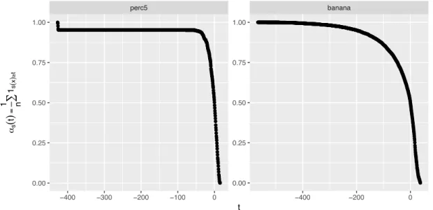
Figure 3 visualizes the behaviour of the empirical mass/probability ˆ–sX,θ(t) depending
on the threshold twith values that lie in the range of the score values S.
● ● ●● ● ● ● ●●●●●●●●●●●●●●●●●●●●●●●●●●●●●●●●●●●●●●●●●●●●●●●●●●●●●●●●●●●●●●●●●●●●●●●●●●●●●●●●●●●●●●●●●●●●●●●●●●●●●●●●●●●●●●●●●●●●●●●●●●●●●●●●●●●●●●●●●●●●●●●●●●●●●●●●●●●●●●●●●●●●●●●●●●●●●●●●●●●●●●●●●●●●●●●●●●●●●●●●●●●●●●●●●●●●●●●●●●●●●●●●●●●●●●●●●●●●●●●●●●●●●●●●●●●●●●●●●●●●●●●●●●●●●●●●●●●●●●●●●●●●●●●●●●●●●●●●●●●●●●●●●●●●●●●●●●●●●●●●●●●●●●●●●●●●●●●●●●●●●●●●●●●●●●●●●●●●●●●●●●●●●●●●●●●●●●●●●●●●●●●●●●●●●●●●●●●●●●●●●●●●●●●●●●●●●●●●●●●●●●●●●●●●●●●●●●●●●●●●●●●●●●●●●●●●●●●●●●●●●●●●●●●●●●●●●●●●●●●●●●●●●●●●●●●●●●●●●●●●●●●●●●●●●●●●●●●●●●●●●●●●●●●●●●●●●●●●●●●●●●●●●●●●●●●●●●●●●●●●●●●●●●●●●●●●●●●●●●●●●●●●●●●●●●●●●●●●●●●●●●●●●●●●●●●●●●●●●●●●●●●●●●●●●●●●●●●●●●●●●●●●●●●●●●●●●●●●●●●●●●●●●●●●●●●●●●●●●●●●●●●●●●●●●●●●●●●●●●●●●●●●●●●●●●●●●●●●●●●●●●●●●●●●●●●●●●●●●●●●●●●●●●●●●●●●●●●●●●●●●●●●●●●●●●●●●●●●●●●●●●●●●●●●●●●●●●●●●●●●●●●●●●●●●●●●●●●●●●●●●●●●●●●●●●●●●●●●●●●●●●●●●●●●●●●●●●●●●●●●●●●●●●●●●●●●●●●●●●●●●●●●●●●●●●●●●●●●●●●●●●●●●●●●●●●●●●●●●●●●●●●●●●●●●●●●●●● ● ● ● ● ●●●●●●●●● ● ● ● ● ●●● ● ●● ● ● ●● ● ● ● ● ● ● ● ●● ● ● ● ● ● ● ●● ● ● ● ●● ● ● ●● ● ● ●●● ● ● ●●●●●●●●●●●●●●●●●●●●●●●●●●●●●●●●●●●●●●●●●●●●●●●●●●●●●●●●●●●●●●●●●●●●●●●●●●●●●●●●●●●●●●●●●●●●●●●●●●●●●●●●●●●●●●●●●●●●●●●●●●●●●●●●●●●●●●●●●●●●●●●●●●●●●●●●●●●●●●●●●●●●●●●●●●●●●●●●●●●●●●●●●●●●●●●●●●●●●●●●●●●●●●●●●●●●●●●●●●●●●●●●●●●●●●●●●●●●●●●●●●●●●●●●●●●●●●●●●●●●●●●●●●●●●●●●●●●●●●●●●●●●●●●●●●●●●●●●●●●●●●●●●●●●●●●●●●●●●●●●●●●●●●●●●●●●●●●●●●●●●●●●●●●●●●●●●●●●●●●●●●●●●●●●●●●●●●●●●●●●●●●●●●●●●●●●●●●●●●●●●●●●●●●●●●●●●●●●●●●●●●●●●●●●●●●●●●●●●●●●●●●●●●●●●●●●●●●●●●●●●●●●●●●●●●●●●●●●●●●●●●●●●●●●●●●●●●●●●●●●●●●●●●●●●●●●●●●●●●●●●●●●●●●●●●●●●●●●●●●●●●●●●●●●●●●●●●●●●●●●●●●●●●●●●●●●●●●●●●●●●●●●●●●●●●●●●●●●●●●●●●●●●●●●●●●●●●●●●●●●●●●●●●●●●●●●●●●●●●●●●●●●●●●●●●●●●●●●●●●●●●●●●●●●●●●●●●●●●●●●●●●●●●●●●●●●●●●●●●●●●●●●●●●●●●●●●●●●●●●●●●●●●●●●●●●●●●●●●●●●●●●●●●●●●●●●●●●●●●●●●●●●●●●●●●●●●●●●●●●●●●●●●●●●●●●●●●●●●●●●●●●●●●●●●●●●●●●●●●●●●●●●●●●●●●●●●●●●●●●●●●●●●●●●●●●●●●●●●●●●●●●●●●●●●●●●●●●●●●●●●●●●●●●●●●●●●●●●●●●●●●●●●●●●●●●●●●●●●●●●●●●●●●●●●●●●●●●●●●●●●● ● ●●●●●●●●● ●●●●● ● ● ● ●● ● ● ●● ● ● ● ●●● ● ●●● ● ●●●●●●●●●●●●●●●●●●●●● perc5 banana −400 −300 −200 −100 0 −400 −200 0 0.00 0.25 0.50 0.75 1.00 0.00 0.25 0.50 0.75 1.00 t αs ( t ) = 1 ∑ n 1s ( x ) ≥ t
Figure 3: Empirical mass/probabilities ˆ–sX,θ, which shows the relative frequency that
the score values are greater than the threshold t. The score values are ex-tracted with the scoring functionsX,θ generated by OC-SVM on the synthetic
data set 5perc (left) and thebanana data set (right) (see Section 8.1 for more information on the data sets).
Figure 3 shows that with increasing thresholdst, the number of score values which are greater than the threshold t (6) are decreasing (less observations classified as normal). So the lower the threshold t the greater is the mass of the data classified as normal. In the left panel of the graphic (5perc data set) one can see that the threshold between
≠250 and≠25 would yield the same mass–sX,θ(t), whereas the right panel of the graphic
(banana data set) shows that themass varies with a varying threshold.
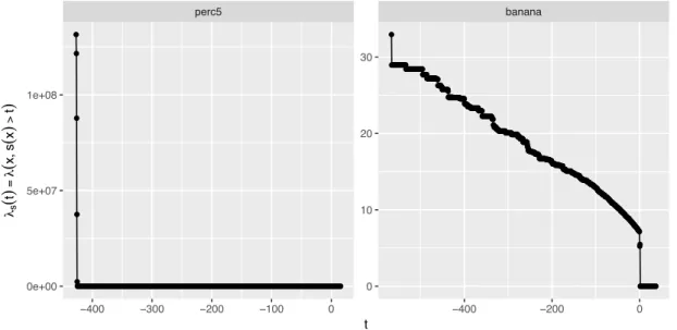
Figure 4 visualizes the behaviour of ⁄sX,θ(t) depending on the threshold t with values
that lie in the range of the score values S.
● ● ● ● ● ● ● ●●●●●●●●●●●●●●●●●●●●●●●●●●●●●●●●●●●●●●●●●●●●●●●●●●●●●●●●●●●●●●●●●●●●●●●●●●●●●●●●●●●●●●●●●●●●●●●●●●●●●●●●●●●●●●●●●●●●●●●●●●●●●●●●●●●●●●●●●●●●●●●●●●●●●●●●●●●●●●●●●●●●●●●●●●●●●●●●●●●●●●●●●●●●●●●●●●●●●●●●●●●●●●●●●●●●●●●●●●●●●●●●●●●●●●●●●●●●●●●●●●●●●●●●●●●●●●●●●●●●●●●●●●●●●●●●●●●●●●●●●●●●●●●●●●●●●●●●●●●●●●●●●●●●●●●●●●●●●●●●●●●●●●●●●●●●●●●●●●●●●●●●●●●●●●●●●●●●●●●●●●●●●●●●●●●●●●●●●●●●●●●●●●●●●●●●●●●●●●●●●●●●●●●●●●●●●●●●●●●●●●●●●●●●●●●●●●●●●●●●●●●●●●●●●●●●●●●●●●●●●●●●●●●●●●●●●●●●●●●●●●●●●●●●●●●●●●●●●●●●●●●●●●●●●●●●●●●●●●●●●●●●●●●●●●●●●●●●●●●●●●●●●●●●●●●●●●●●●●●●●●●●●●●●●●●●●●●●●●●●●●●●●●●●●●●●●●●●●●●●●●●●●●●●●●●●●●●●●●●●●●●●●●●●●●●●●●●●●●●●●●●●●●●●●●●●●●●●●●●●●●●●●●●●●●●●●●●●●●●●●●●●●●●●●●●●●●●●●●●●●●●●●●●●●●●●●●●●●●●●●●●●●●●●●●●●●●●●●●●●●●●●●●●●●●●●●●●●●●●●●●●●●●●●●●●●●●●●●●●●●●●●●●●●●●●●●●●●●●●●●●●●●●●●●●●●●●●●●●●●●●●●●●●●●●●●●●●●●●●●●●●●●●●●●●●●●●●●●●●●●●●●●●●●●●●●●●●●●●●●●●●●●●●●●●●●●●●●●●●●●●●●●●●●●●●●●●●●●●●●●●●●●●●●●●●●●●●●●●●●●●●●●●●●●●●●●●●●●●●●●●●●●●●●●●●●●●●●●●●●●●●●●●●●●●●●● ● ●●●●●●●●●●●●●●●●●●●●●●●●●●●●●●●●●●●●●●●●●●●●●●●●●●●●●●●●●●●●●●●●●●●●●●●●●●●●●●●●●●●●●●●●●●●●●●●●●●●●●●●●●●●●●●●●●●●●● ● ● ●●●●●●●●●●●●●● ● ● ● ●●●●●●●●●●●●●●●●●●●●●●●●●●●●●●●●●●●●●●● ● ● ●●●●●●●●●●●●●●●●●●●●●●●●●●●●●●●●●●●●● ●●●●●●●●●●●●●●●●●●●●●●●●●●●●●●●●●●●●●●●●●●●●●●●●●●●●●●●●●●●●●● ● ● ● ● ●●●●●●●●●●●●●●●●●●●●●●●●●●●●●●●●●●●●●●●●●●●●●●●●●●●●●●●●●●●●●● ● ● ● ●●●●●●●●●●●●●●●●●●●●●●●●●●●●●●●●●●●●●●● ● ● ●●●●●●●●●●●●●●●●●●●●●●●●●●●●●●●●●●●●●●●●●●●●●●●●●●●●●●●●●●●●●●●●●●●●●●●●●●●●●●●●●●●●●●●●●●●●●●●●●●● ●●●●●●●●●●●●●●●●●●●●●●●●●●● ● ●●●● ● ●●●●●●●●●●●●●●●●●●●●●●●●●●●●●●●●●●●●●●●●●●●●●●●●●●●●●●●●●●●●●●●●●●●●●●●●●●●●●●●●●●●●●●●●●●●●●●●●●●●●●●●●●●●●●●●●●●●●●●●●●●●●●●●●●●●●●●●●●●●●●●●●●●●●●●●●●●●●●●●●●●●●●●●●●●●●●●●●●●●●●●●●●●●●●●●●●●●●●●●●●●●●●●●●●●●●●●●●●●●●●●●●●●●●●●●●●●●●●●●●●●●●●●●●●●●●●●●●●●●●●●●●●●●●●●●●●●●●●●●●●●●●●●●●●●●●●●●●●●●●●●●●●●●●●●●●●●●●●●●●●●●●●●●●●●●●●●●●●●●●●●●●●●●●●●●●●●●●●●●●●●●●●●●●●●●●●●●●●●●●●●●●●●●●●●●●●●●●●●●●●●●●●●●●●●●●●●●●●●● ● ● ● ●●●●●●●●●●●●●●●●●●●●●●●●●●●●●●●●●●●●●●●●●●●●●●●●●●●●●●●●●●● perc5 banana −400 −300 −200 −100 0 −400 −200 0 0 10 20 30 0e+00 5e+07 1e+08 t λs ( t ) = λ ( x , s ( x ) > t )
Figure 4: Lebesgue measure or volume ⁄sX,θ of the subset of x values for which the
corresponding score value si is greater than the thresholdt. The score values are extracted with the scoring function sX,θ generated by OC-SVM on the
synthetic data set5perc(left) and thebanana data set (right); (see Section 8.1 for more information on the data sets).
Figure 4 shows, that with increasing threshold t the volume ⁄sX,θ (5) decreases, as
less score values exceed threshold t. Therefore, the set{x, sX,θ(X) Øt} for calculating
the volume is smaller.
Thus, with increasing threshold t, both, the mass and the volume in the Mass Volume curve definition are decreasing.
The definition of the MV curve up to this point has a two-dimensional output. If the mass–sX,θ(t) has no flat parts, which means that its derivatives are non-zero at a given
point [Glaister, 1991], than the MV curve can be defined as
M V CsX,θ :–œ[0,1)‘æ⁄sX,θ(– ≠1
where the inverse of–sX,θ(t) is defined as
–≠s1
X,θ(–) = inf{tœR,–sX,θ(t)Æ–} (8)
The curve of–≠sX,1θ(–) is shown in Figure 5.
●●●●●●●●●●●●●●●●●●●● ●●●●●●●●●●●●●●●●●●●●●●●●●●●●● ●●●●●●●●●●●●● ●●●●●●● ●●●●●● ●●●● ●● ●● ●● ●● ● ● ● ● ● ● ● ● ● ● ● ● ●●●●●●●●●●●●●●●●●●●●●●●●●●●●●●●●●●●●●●●●●●●●●●●●●●●●●●●●●●●●●●●●● ●●●●●●●●●●●●●●●●●●●●●●●● ●●●●● ● ●●●● banana perc5 0.00 0.25 0.50 0.75 1.00 0.00 0.25 0.50 0.75 1.00 −400 −300 −200 −100 0 −300 −200 −100 0 α αs − 1 ( α ) = inf t ∈ R , αs ( t ) < α
Threshold, for which the Mass of P(s(x)>t) is α
Figure 5: The inverse function of–sX,θ(t) is – ≠1
sX,θ(t) and is based on score values, which
are extracted with the scoring function sX,θ generated by OC-SVM on the
synthetic data set5perc(left) and thebanana data set (right); (see Section 8.1 for more information on the data sets).
As stated above the true density f is unknown, therefore we need to define the em-pirical MV curve of a scoring function, given X and the empirical ˆ–sX,θ(t):
\
M V CsX,θ :–œ[0,1)‘æ⁄sX,θ( ˆ– ≠1
sX,θ(–)) (9)
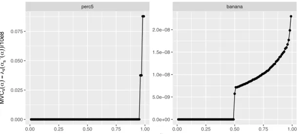
●●●●●●●●●●●●●●●●●●●●●●●●●●●●●●●●●●●●●●●●●●●●●●●●●●●●●●●●●●●●●●●●●●●●●●●●●●●●●●●●●●●●●●●●●●●●●●● ●● ●● ●●●●●●●●●●●●●●●●●●●●●●●●●●●●●●●●●●●●●●●●●●●●●●●●● ● ●●●●●●● ●●●●● ●●●●●● ●●●● ●●●● ●●●● ●●● ●● ●●● ●● ●● ● ●● ● ● ● ● perc5 banana 0.00 0.25 0.50 0.75 1.00 0.00 0.25 0.50 0.75 1.00 0.0e+00 5.0e−09 1.0e−08 1.5e−08 2.0e−08 0.000 0.025 0.050 0.075 α M V Cs ( α ) = λs ( αs − 1 ( α )) /10e8 MVC dependence on α values
Figure 6: TheM VsX,θ(α)based on score values that are extracted with an OC-SVM from
the synthetic data set5perc (left) and thebanana data set (right); (see Section 8.1 for more information on the data sets).
Figure 6 shows, the higher the mass – of the normal data, the larger is the value of the MV curve.
The output of the M V CsX,θ characterizes the underlying score function sX,θ from an
anomaly detection algorithm at a given mass – i.e. it returns a performance measure forsX,θ when the mass of the normal data is assumed to be–.
Moreover the MV curve can be used to compare different score functions and anomaly detection algorithms at a given mass point–. Optimal scoring functions have MV curves that are minimal everywhere according to Clémençon and Jakubowicz [2013, p.4]. In the paper it is stated that ifs1 ands2are two scoring functions onX, than the ordering provided bys1 is better than that provided by s2 when
’–œ[0,1)M V Cs1(–)ÆM V Cs2(–) (10) Furthermore Clémençon and Jakubowicz [2013, p.4] provide a proposition about the optimal MV curve, which is the M V Cf curve based on the true density f(x) of the random variable X. As the true density f(x) is not known, the optimal MC curve should be based on the optimal scoring function, that ranks the observations X in the same order asf(X), i.e., a strictly increasing transformation off(X). The set of optimal scoring functions is then defined as
Sú ={T ¶f : T :Imf(X)æR
+,strictly increasing} (11)