Working Paper 10-31 Departamento de Economía de la Empresa Business Economic Series 05 Universidad Carlos III de Madrid
September 2010 Calle Madrid, 126
28903 Getafe (Spain)
Fax (34-91) 6249607
SYSTEMIC RISK MEASURES: THE SIMPLER THE
BETTER?
∗María Rodrígez-Moreno1 and Juan Ignacio Peña 2
Abstract
We compute six different sets of systemic risk measures for a sample of the 20 biggest European and 13 biggest US banks from January 2004 to November 2009. The six measures are based on i) Principal components of the bank’s Credit Default Swaps (CDSs), ii) Interbank interest rate spreads, iii) Structural credit risk models, iv) Collateralized Debt Obligations (CDOs) indexes and their tranches, v) Multivariate densities computed from CDS spreads and vi) Co-Risk measures. We then rank the measures using three different criteria: i) Causality tests, ii) Price discovery tests and iii) their correlation with an index of systemic events. For the European and US markets, the best indicators are the first Principal Component of the single-name CDSs and the LIBOR-OIS or LIBOR-TBILL spreads, respectively, whereas the least reliable indicators are the Co-Risk measures and the systemic spreads extracted from the CDO indexes and their tranches.
Keywords:Systemic Risk; CDS; Libor spreads; CoVaR
JEL Classification:C32, G01, G15, G21
1
University Carlos III of Madrid, Department of Business Administration, [email protected] 2
1. Introduction
The financial system plays a fundamental role in the global economy as the middleman between agents who need to borrow and agents who are willing to lend or invest. As a consequence, it is naturally linked to all economic sectors and therefore, if the financial system does not work properly, its problems have a strong impact on the real economy. For instance, in the current crisis, the total cost to G-20 countries of the bail-out of the financial system is around $10.8 trillion as of September 2009.1 However, the cost of the crisis is not
limited to the bail-outs. Substantial costs are also incurred by the negative evolution of the fundamental macro variables such as GDP growth rate, unemployment rates and government deficits, among others. For instance, the annual GDP growth rate2 decreased from 3.09% in 2007 to -4.09% in 2009 in the European Union. In the US, this rate decreased from 2.14% to -2.45%. With respect to the unemployment rate, it increased from 7.8% in January 2007 to 9.4% in November 2009 in the European Union. In the US, this rate increased from 4.6% to 10% in the same period. Regarding the government deficits3, they dramatically increased from 0.8% in 2007 to 6.7% in 2009 in the European Union, and in the same period, US government deficits increased from 1.14% to 9.9%.
As many of these problems come from events related with systemic risk propagating from the banking sector to the real economy, it is important to understand the relationship among measures of systemic risk and give an indication of the relative usefulness of the available measures. This papers aims to shed some light on these pressing issues by means of an
1 The BBC stated on 10September 2009 that according to IMF data, G-20 countries have spent $10.8 trillion.
However, most of the bail-outs are in the form of guarantees to the financial system and hence, governments hope to recover some of the money. http://news.bbc.co.uk/2/hi/business/8248434.stm. Concretely, the IMF estimated global losses to be around $3.4 trillion by October 2009. http://www.imf.org/external/pubs/ft/gfsr/2009/02/pdf/press.pdf
2 Annual percentages of constant price GDP are year-on-year changes.
empirical analysis of the most widely used and well-known measures of systemic risk employed by investors and regulators worldwide.
Acharya and Richardson (2009) discuss the factors causing the near collapse of the global financial system (mainly the combination of a credit boom and a housing bubble) and give several proposals for regulatory reform. Regarding systemic risk, they propose a definition of systemic risk which involves its effect on the real economy and a device for reducing it through taxation.4 Following a similar approach, Brunnermeier (2009) presents a description of the “originate and distribute” model and an event logbook of the crisis for the period 2007-2008. In an environment of mild economic conditions, financial institutions have taken advantage of many financial innovations (e.g., Credit Default Swaps or Collateralized Debt Obligations, among others), some of them very complex and with unexpected downside effects in scenarios of financial distress. Nonetheless, the problem is not only that the financial system is in trouble during the crisis but the whole economy is also affected. This relationship and the search for the best performing systemic risk measure is our basic motivation for addressing the relative performance of the available systemic risk measures. Billio, Gertmansnki, Lo and Pelizzon (2010) use monthly data to study the interconnectedness among the returns of hedge funds, banks, brokers, and insurance companies but they use only two measures: principal components analysis and Granger-causality tests. They find that all four sectors have become highly interrelated over the past decade, possibly increasing the level of systemic risk in the finance and insurance industries, and they suggest that hedge funds can provide early indications of market dislocation.
In this paper, we concentrate on what are widely acknowledged to be the most important systemic actors: the biggest banks in the two biggest economic areas (the European Union
4These ideas are extended in other papers: Acharya, Pedersen, Philippon and Richardson (2010a and
and the US).5 We employ daily data and we compare a comprehensive set of measures. Specifically, we compute six different sets of systemic risk measures for a sample of the 20 biggest European and 13 biggest US banks from January 2004 to November 2009.6 The six measures are based on i) Principal components of the bank’s Credit Default Swaps (CDSs), ii) Interbank interest rates, iii) Structural (Merton (1973)) credit risk models, iv) Collateralized Debt Obligations (CDOs) indexes and their tranches v) Multivariate densities computed from CDS spreads and vi) Co-Risk measures. We then compare them using three different criteria: i) Causality tests, ii) Price discovery test, and iii) their correlation with an index of systemic events.
Our main empirical findings are as follows. For the European market, the best indicator is the LIBOR-OIS spread followed by the first Principal Component of the single-name CDSs whereas the least reliable indicator is the Delta Co-Expected Shortfall. For the US market, the best indicator is the first Principal Component of the single-name CDSs followed by the spread LIBOR-TBILL, whereas the least reliable indicator is the systemic spread extracted from the CDO indexes and their tranches.
Therefore, our results imply that the better performing measures of systemic risk are based on simple indicators obtained from credit derivatives and interbank markets. On the other hand, indicators relying on structural models or complex statistical procedures do not perform particularly well in our sample. The implications for investors and regulators are straightforward. Look for simple, robust indicators based directly on liquid market prices and be aware of overcomplicated modelling based on dubious assumptions and of the inferences from the prices of financial products traded in thin markets.
5
Billio et al. (2010) find that banks may be more central to systemic risk than non-bank financial institutions that engage in banking functions.
6 In a recent study, the International Monetary Fund (2009) posits that smaller institutions may also contribute
to systemic risk if they are closely interconnected. However, systemic risk should be most readily observed in the largest banks.
This paper is divided into 6 sections. Section 2 reviews the literature. In Section 3, we give a brief description of the dataset employed in our analysis. Section 4 describes the different measures of systemic risk proposed in the extant literature. This section also includes the estimation of these measures using our database. In Section 5, we compare these measures among groups and run a “horse race” among them using three different criteria. Section 6 concludes.
2. Literature Review
There is no general agreement on the definition of systemic risk.7 De Bandt and Hartmann (2002) survey theoretical and empirical approaches and define systemic risk as a “systemic event that affects a considerable number of financial institutions or markets, thereby severely impairing the general well-functioning of the financial system”. A different approach is taken by Kaufman (2000) and Kaufman and Scott (2003), who define systemic risk as “the risk or probability of breakdown in an entire system and it is evidenced by co-movements (correlations) among most or all the parts”. They assign the most frequent concepts about systemic risk to three groups: macro shocks, micro level and spillover effects though indirect interconnections. Billio et al. (2010) state that “Systemic risk can be defined as the probability that a series of correlated defaults among financial institutions, occurring over a short time span, will trigger a withdrawal of liquidity and widespread loss of confidence in the financial system as a whole”. Recently, the Financial Stability Report of ECB (December 2009) classified theoretical and empirical papers about systemic risk into three categories: contagion, macro shocks and unwinding of imbalances.
Although the definition of systemic risk diverges among papers, the common factor is the generalized distress of financial institutions, which makes it difficult for the financial system
7 In the Global Financial Stability Report by the IMF (2009), it is recognized that systemic risk is a term
to perform well. On the basis of this characteristic, we define systemic risk as the risk of suffering an adverse effect on the real economy derived from the malfunctioning of the financial sector. Clearly, the worse is the situation in the financial system, the stronger is the systemic risk, although this relationship is not necessarily linear.
Until recently, academic research has mainly focused on measuring idiosyncratic and systematic risk, ignoring, at least in part, the importance of systemic risk. For instance, for the case of the banking industry, the Basel I (1988) and Basel II (2004) Accords design risk management policy on the basis of the banks’ portfolios, ignoring interconnection among banks. Therefore, no provision for systemic risk is included in the current regulatory framework.
Interest in systemic risk is relatively new. At the end of the 1990s, concern about the stability of the international financial system increased as a consequence of the crisis in Mexico (1994), Asia (1997), Russia (1998) and Brazil (1999).8
Nevertheless, systemic risk measures have attracted more attention in recent years. Going beyond traditional approaches based on pure contagion, new dimensions of systemic risk have been developed. These dimensions are related to interconnections to common factors. Researchers realize that the rise in the complexity and globalization of financial services has contributed to establishing strong interconnections among financial institutions. In this vein, credit derivatives like CDOs and CDSs have played a crucial role, in part because they are new products which are traded in bilateral transactions Over-The-Counter (OTC), and as result, they involve greater counterparty risk and less transparency. As a consequence, the disquiet about systemic risk has been growing as well as the notional value of
8 This disquiet was voiced by none other than Alan Greenspan, chairman of the Federal Reserve (1986-2006):
“Second only to its macrostability responsibilities is the central bank's responsibility to use its authority and expertise to forestall financial crises (including systemic disturbances in the banking system) and to manage such crises once they occur.”
outstanding CDSs and CDOs.9 In fact, the relationship between these credit derivatives and economy-wide risk has already been documented in the literature (see Mayordomo and Peña, 2010).
Regarding the measurement of systemic risk, two complementary approaches, macro and
micro, can be employed. The macro or aggregated approach focuses on the evolution of
macro indicators in order to detect possible bubbles in the economy. Some examples of this approach are Borio and Lowe (2002a, 2002b and 2004) and Borio and Drehmann (2009), who propose to measure the financial unwinding of imbalances by means of price misalignments in some key indicators like inflation-adjusted equity prices or private sector leverage. The micro approach focuses on the individual institutions’ financial health to
determine the level of systemic risk in the economy (i.e., portfolio) by means of analyzing both market and accounting information. In this paper, we focus mainly on the micro level, analyzing the market information provided by individual institutions. The macro level is also studied by means of the interest rates. In any case, we realize that both approaches are complementary to each other.
Although some papers have addressed the problem of systemic risk10, few of them propose measures that allow surveillance institutions to monitor the aggregate level of the systemic risk and its concentration in key financial intermediaries. These measures could play a relevant role as leading indicators of future impending crises. Lehar (2005) proposes extracting systemic risk measures on the basis of Merton’s model (1973). Using Monte Carlo simulations, the author proposes a measure of systemic risk which is based on the probability that banks with total assets of more than a certain percentage ε of all banks’
9 To give an example, the outstanding notional amount of CDS was $8.42 trillion at the end of 2004 and $62.2
trillion at the end of 2007. Once the subprime crises broke out, the outstanding notional amount decreased to $38.6 trillion at the end of 2008 (source ISDA).
10 See Bartram, Brown and Hund (2005), who analyze the global banking system through event study
methodology; Brühler and Prokopczuk (2007), who analyze tail dependence of stock returns by means of an
Archimedean copula; andAvesani, García and Li (2006), who construct an indicator for sector surveillance
assets go bankrupt within a short period of time. Additionally, the author proposes a similar measure of systemic risk as the probability that more than a certain fraction of all banks go bankrupt at the same time. Allenspach and Monnin (2007) improve Lehar’s measure by estimating, through a structural model, the banks’ asset-to-debt ratio. As an alternative to structural models, other authors employ CDSs to measure systemic risk. Bhansali, Gingrich and Longstaff (2008) extract the idiosyncratic, systematic and systemic risks from U.S (CDX) and European (iTraxx) prices of indexed credit derivatives by means of a linearized three-jump model. Huang, Zhou and Zhou (2009) propose creating a synthetic CDO whose underlying portfolio consists of debt instruments issued by banks to measure the systemic risk of the banking system through the spread of the tranche that captures losses higher than 15%. Segoviano and Goodhart (2009) propose a set of banking stability measures11 based on distress dependence, which is estimated by the Banking System Multivariate Density (BSMD). Their procedure for estimating the multidensity function (CIMDO-copula) is able to capture both linear and non-linear distress dependences and allows changes throughout the economic cycle.12 Finally, Adrian and Brunnermeier (2008) propose a set of “co-risk management” measures based on traditional management tools. They estimate the institution i’s Co-Value-at-Risk (CoVaRi) as the whole system (i.e., portfolio)’s
Value-at-Risk (VaRs) conditioned on institution i being in distress (i.e., being at its unconditional VaRilevel). On the basis of CoVaR, they calculate the marginal contribution of institution i
to the overall systemic risk as the difference between CoVaR and the unconditional whole
system’s VaR, which we denoted asΔCoVaRi.
In this article, we shed light on the relative quality of the aforementioned measures, comparing them by using three different criteria in the context of the current financial crisis.
11 The authors propose three different categories of measures: (a) common distress in the banks of the system;
(b) distress between specific banks; (c) distress in the system associated with a specific bank.
12 By means of CIMDO-copula, the authors overcome the drawbacks of the characterization of distress
dependence of financial returns with correlations, which has been one of the most popular approaches for
3. Dataset
Our analysis of systemic risk is based on two portfolios which contain the largest western Europe (including non-Eurozone) and United States (US) banks. Regarding the former portfolio, we select the largest western European banks according to the “The Banker” ranking for which we have information about CDS spreads, liabilities and equity prices. With respect to the US bank portfolio, we select the largest US banks according to the FED ranking13 for which we have information about CDS spreads, liabilities and equity prices.
Our final sample is composed of 20 European banks and 13 US banks and is summarized in Table 1, which also contains the average portfolio weights on the basis of their market capitalization during the sample period.
The main inputs of the measures are single-name CDS spreads, liabilities and equity prices. The CDS spreads and equity prices are reported on a daily basis (end of day) while the liabilities are reported on annual terms. These variables are obtained either from Reuters or DataStream depending on the data availability in both data sources. Additionally, other variables are required. For instance, the 3-month and 10-year LIBOR, swap rates and treasury yields are needed. We employ interest rates from the two economic areas: US and the Eurozone.14, 15 These variables are obtained from Reuters. Moreover, CDO index
spreads are also employed: the US CDO index Investment Grade (IG) spreads (CDX IG 5y) and the European one (iTraxx IG 5y) as well as their tranches. The CDX index has six tranches with attach and detach points at 0%, 3%, 7%, 10%, 15%, 30% and 100% while the
13 In both cases, we require the bank to have been included in the top 25 and 40 of the list of western Europe
and US banks, respectively, at least once between 2004 and 2009. Banks that have been taken over or gone bankrupt are employed until the moment when such events happened.
14 Reuters uses French government bonds as the benchmark for the Eurozone up to 05/08/2010. After that date,
German government bonds are the benchmark.
15 Our western European portfolio is composed of Eurozone and non-Eurozone banks (i.e., Denmark, Sweden,
Switzerland and the UK). Regarding the second group, we also analyzed the UK’s Libor spreads because of the global importance of that financial system. However, analysis of UK spreads does not add additional information to Eurozone spreads.
iTraxx has also six tranches with attach and detach points at 0%, 3%, 6%, 9%, 12%, 22% and 100%. Those index spreads for the different tranches are gathered from Markit.
The sample spans from January 1, 2004 to November 4, 2009. This sample period allows us to study the behavior of the systemic risk measures in both pre-crisis and crisis periods because August 2007 is commonly considered the starting point of the sub-prime crisis. However, the sample period used for the CDO indexes is slightly shorter. Concretely, CDX IG 5y spans from March 2006 to November 2009 while iTraxx IG 5y spans from March 2005 to November 2009 due to the lack of data at the beginning of the sample period. During certain periods of the crisis, the on-the-roll (i.e., the one that corresponds to the current index’s series and version) market is dried out and no spreads are available. In these cases, we replace them with the closest available out-the-roll series spreads.
4. Measures
In this section, we briefly summarize the systemic risk measures which are proposed in the literature and based on market information and report our estimation for these measures using our dataset. We classify those measures into six different groups: (i) based on a Principal Component Analysis (PCA) of CDS spreads; (ii) based on interbank interest rates; (iii) based on structural models; (iv) based on the Collateralized Debt Obligations (CDO) indexes and their tranches; (v) based on multivariate densities which are recovered through CDS spreads; (vi) based on “co-risk management” measures such as Delta CoVaR.16
16 “Co-risk management” measures refer to the conditional, co-movement or even contagion measures which
a. PCA of CDS
CDSs are credit derivatives that provide insurance against the risk of default of a certain company (“name”), and hence, their spreads measure the risk that is faced by bondholders of the reference entity.
The first measure that we implement consists of performing a Principal Component Analysis (PCA) on a pool of the CDS spreads. Longstaff and Rajan (2007) analyze the CDS spreads of the components of the CDX index. They find that there is a dominant factor that mainly drives the spreads across all industries, which is consistent with the existence of an economy-wide or systemic risk component.
In our sample, we find that 93% and 90% of the bank’s CDSs variance is explained by the first Principal Component Factor (PCF) in European and US banks, respectively, in agreement with Longstaff and Rajan (2008).
Figure 1 shows the evolution of both principal components during the whole sample period. From January 2004 to July 2007, both components remain almost flat. When the crisis starts in August 2007, and until March 2009, both variables follow an upward trend in which three peaks are clearly noticeable: March 2008, September 2008 and March 2009.17 Both factors are largely similar but in the period from September 2008 to December 2008, which corresponds to a period of high stress in the US markets after the bankruptcy of the Lehman Brothers, the US factor is higher. After March 2009, both variables decrease noticeably and at the end of the sample period, the levels of these variables return to a level similar to the one at the beginning of 2008, but still clearly above their pre-crisis levels.
17 The first two peaks coincide with the Bear Stearns and Lehman Brothers episodes. Regarding the last one,
there is not a clear reason as in the previous cases, although we guess that it is due to huge losses of the insurance giant AIG which were publically reported on March 2, 2009, and were the largest quarterly loss in US corporate history.
The first principal components are highly correlated with all banks’ CDS. In the European (US) case, the highest correlation is 0.98 (0.98) with respect to BBVA (State Street Corp) and the lowest is 0.84 (0.85) with respect to Fortis (Capital One FC).
b. Libor Spreads
The second group of systemic risk measures involves the use of the LIBOR18 as the reference interest rate relative to either the Overnight Interest Swap (OIS) or Treasury bills (TBill)19, usually known in the literature as LIBOR spreads.20 The first measure is defined as the difference between the 3-month LIBOR rate and the 3-month Overnight Interest Swap (OIS). The second measure is defined as the difference between the 3-month LIBOR rate and 3-month Treasury bills. These measures are employed by Brunnermeier (2009) to describe the event logbook of the current crisis and by the Global Financial Stability Report by the IMF (2009), among others.
These two proxies of systemic risk are similar, but important conceptual differences appear between them. The LIBOR represents the unsecured interest rate at which banks lend money to other banks which satisfy certain creditworthiness criteria. Typically, the banks’ credit rating must be at least AA. LIBOR is not totally free of credit risk because it reflects liquidity risk and the bank’s default risk over the following months. On the other hand, OIS is equivalent to the average of the overnight interest rates expected until maturity. It is almost riskless and hence it is not subject to pressures associated with those risks. Therefore, LIBOR minus OIS, or LIBOR-OIS (LO henceforth), reflects liquidity and default risk over the following months. In tranquil periods, this measure should be very low because AA
18 We use the LIBOR for the main currencies under study (i.e., USD LIBOR and EURIBOR, obtained from
Reuters).
19 In Section 3, we work with Eurozone Treasury bills. We repeated the analysis of this section, using German
Treasury bills as a benchmark, and results did not change significantly.
20 These measures do not directly refer to the individual financial institution’s financial health, but give
credit rating institutions should not have either significant liquidity risk or default risk. However, in periods of turmoil, this spread should widen so as to capture these risks.
LIBOR minus Treasury bill or LIBOR-TBILL (LT henceforth) is the second systemic risk measure considered in this section. Treasury bill rates are the rates that an investor earns on Treasury bills. In times of crisis, most lenders only accept Treasuries as collateral, pushing down Treasury rates. Hence, LT captures not only liquidity and default risk but also the additional fact that, during periods of turmoil, investors lend against Treasury bills (the best form of collateral), measuring the “flight to quality” effect. In tranquil periods, LT should be very low, while in periods of turmoil, this spread should be larger. Additionally, we
computed what we name the “Natives Are Restless Factor” (NARF)21, namely, the
difference between the LT and LO spreads (or, equivalently, the OIS-TBILL difference). In normal times, the NARF should be close to zero. However, when investors feel growing disquiet because of an unexpected increase in market uncertainty, they are more willing to pay an extra amount to buy the supposedly safer government securities (lowering their yields) and then the NARF increases.
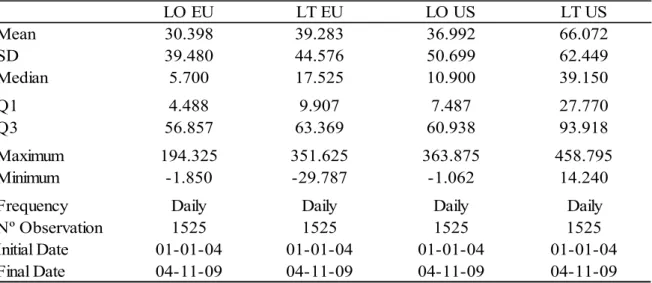
Figure 2 depicts the evolution of the Libor spreads and the dashed area shows the size of the NARF. Panel A refers to the Eurozone (EU) and Panel B refers to the United States (US). The difference between the pre-crisis and crisis periods is clearly seen. The first period is characterized by low and almost constant spreads. These spreads are lower than 10 basis points (b.p.) with the exception of the US LT, which remains around the 30 b.p. line. Note that this Libor spread starts an upward movement by May 2007, while other spreads remain unchanged up to August 2007. The reason could be associated with the role that Treasury bills play as collateral.22
21 This phrase was famously used in “The Island of Lost Souls”, a 1933 film based on the H.G. Wells novel
“The Island of Doctor Moreau”.
22 In May 2007, UBS shut down its internal hedge fund Dillion Read after suffering some large subprime
Since the subprime crisis started on August 2007, two phases of the crisis can be distinguished. The first phase spans from August 2007 to August 2008. It is characterized by a general increment in both the mean level of the spreads around 55 b.p. and high volatility. Like before, the US LT reacts earlier and in a more volatile way in comparison with the other spreads. The second phase of the crisis starts by a generalized jump after the Lehman Brothers bankruptcy.23 The US LT hits up to 458 b.p. followed by the US LO by 363 b.p. (see Table 2, which contains their descriptive statistics). Regarding the NARF, we observe some differences between the Eurozone and the US. The former is almost zero up to the Lehman episode. In the latter, a there is a perceptible level of disquiet that grew substantially from July 2007 to the Lehman episode. After that episode, all spreads followed a downward trend, ending the sample period at pre-crisis levels. This behavior may be related to the announcement of generalized bail-out plans and the very lax stance of the monetary policy.
The main advantage of these measures is that they are easy and quick to compute and could provide some intuition about the evolution of the systemic risk among banks. However, it is important to keep in mind that short term rates are policy targets in the current framework of the monetary policy applied in both Europe and the US and therefore may be subject to external pressures.24
c. Structural Models
The third group of measures is based on the framework of Merton’s model (1973). The basic reference is Lehar (2005) although other authors like Allenspach et al. (2007), Chan-Lau and Kong (2004) or Gray, Merton, and Bodie (2008) use similar approaches.
23 The Lehman Brother bankruptcy sparked off a wave of bankruptcies and bail-outs in the US and Europe.
See Appendix A1 for other events during that period.
24 For example, the Federal Reserve introduced the Term Auction Facility (TAF) on 12 December 2007 with
Lehar (2005) and Elsinger, Lehar and Summer (2006) propose a systemic risk measure based on the probability of default of a given proportion of the banks in a given financial system. The probability of default is linked to the relationship between the banks’ asset value and their liabilities. In summary, the procedure to estimate this variable consists of recovering the bank’s asset values and correlations through Merton’s model and an Exponential Weighted Moving Average (EWMA) model, respectively. Then a simulation is carried out to infer future bank values and compare them with their liabilities according to different criteria in order to construct the systemic risk index: SIV and SIN, which refer to a Systemic risk Index based on the Value of assets and Number of defaulted banks, respectively.
Under Merton’s framework, the bank’s asset value (V) follows a Geometric Brownian
motion with drift μt and volatility σt:
dVt=μtVtdt+σtVtdz (1) The equity Etcan be seen as a call option on the bank’s assets with a strike price equal to
the face value of the bank’s debt Btwhich matures at T. Equity (Et) is given by
Et =VtN(dt)−BtN(dt−σt T) (2) where T T B V d t t t t t σ σ /2) ( ) / ln( + 2
= . This model presents two unknowns (Vt andσt) and only
one equation; therefore, an additional one is needed. In order to solve this problem, we follow Duan’s methodology (Duan, 1994, 2000).25 In both studies, he proposes the following likelihood function:
25 In the literature, two alternatives have been proposed. Ronn and Verma (1986) use a framework based on the
relationship between equity and asset volatility while Duan (1994, 2000) employs a maximum likelihood framework. Lehar (2005, 2006) follows Duan’s methodology because it is consistent with Merton’s model while the other one is not.
(
)
( )
( )
( )
( )
( )
∑
∑
∑
= − = = ⎥ ⎥ ⎦ ⎤ ⎢ ⎢ ⎣ ⎡ − ⎟⎟ ⎠ ⎞ ⎜⎜ ⎝ ⎛ − − − − − − − = m t t t t t t t m t t t m t t t t t t t V V d N V m m E L 2 2 1 2 2 2 2 ˆ ˆ ln 2 1 ˆ ln ˆ ln ln 2 1 2 ln 2 1 , , μ σ σ σ σ σ π σ μ (3)where Vˆt
( )
σt is the solution on Vt of Equation (2) while dˆt corresponds to dtin Equation (3). For each week in the sample period26, parameters μt and σt are estimated, assuming thatthe maturity of the debt is one year (time until the next audit of the bank). To estimate each pair of parameters, we apply a rolling window with a length equal to 104 observations (i.e.,
104
=
m represents two years of observations). For a given week, parameters μt and σt are
estimated on the basis of the last 104 observations of market capitalizations (Et) and total
liabilities (Bt).
27, 28 Then we obtain
( )
σt
Vˆ from Equation (2), using the estimated parameters such that at the end we have a time series of the banks’ asset values.
Subsequently, we estimate the covariance between banks’ asset values to construct the variance-covariance matrix. For this purpose, we employ the Exponential Weighted Moving Average (EWMA) model:
⎟⎟ ⎠ ⎞ ⎜ ⎜ ⎝ ⎛ ⎟ ⎟ ⎠ ⎞ ⎜ ⎜ ⎝ ⎛ − + = − − − 1 , , 1 , , 1 , , (1 )log log t j t j t i t i t ij t ij V V V V λ λσ σ (4)
Following the practice in the RiskMetrics framework, parameter λ is set equal to 0.94. This methodology enables us to estimate a variance-covariance matrix (Σt) for each period. This
matrix is employed to predict the future value of the bank by means of Monte Carlo simulations. The underlying idea is that firm asset values can be modelled through a
26 Parameters are estimated on a weekly basis. Lehar estimates those parameters on a monthly and yearly basis
in 2005 and 2006, respectively.
27 Using total liabilities of the firm implies that all the debt is insured. Although this is a simplification, given
the bailout practices, this could be a reasonable assumption,as Laeven (2008) states.
28 Regarding total liabilities, data is available yearly and has been transformed by linear interpolation into
weekly data. Similar procedures are also employed by Allenspach et al. (2006) and Chan-Lau et al. (2004), who transform the series by either linear or quadratic interpolation to monthly data.
multivariate Geometric Brownian motion. By means of Ito’s Lemma, the evolution of Vt
can be defined as:
⎭ ⎬ ⎫ ⎩ ⎨ ⎧ + − =V T T X VT 2 exp 2 0 σ μ (5) whereX =Nm
( )
0,I uand u is obtained by Cholesky Decomposition of thevariance-covariance matrix (i.e.Σ =u'u). Hence, for each week, we obtain Vt, σt and μt, which come
from Merton’s model. After that, we simulate 50,000 multinomial normal distributions with a distribution function following a Normal distributionNm
( )
0,I for each period to simulatedifferent paths of V.29
The systemic risk measure is computed as the probability that banks with total assets of more than a given percentage (ε) of all bank assets go bankrupt. Formally,
∑
∑
∈ ∈ + + < ∀ ∈ ⊂ < F i t i J j t j t j t j B j J F V V V , 1 , 1 , , ξ , (6)where Vj,t+1 is the value that we have already simulated, while we consider Bj,t+1= Bj,t. This
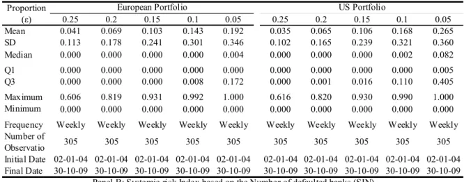
measure is called SIV. Figure 3 depicts the probability that 5, 10 and 15, 20 and 25% (i.e., five different values for ε) of the all considered banks go bankrupt for the next six months in the European (Panel A) and US (Panel B) banking system. In general, European and US systemic risk measures behave in a similar way. Before 2008, those measures were zero or almost zero for all ε, although the smallest one (i.e.,ε =0.05),albeit different from zero, is usually at very low levels.30 Since the summer of 2008, a year after the subprime crisis started, those probabilities increased sharply. European measures jumped noticeably to a high level up to March 2009. After this date, there was a downward trend. On the contrary, US measures have followed a smoothly increasing trend and have maintained a similar level since October 2008. Table 3 contains the descriptive statistics for those measures. As can be
29 See Lehar (2005) for the details of the simulation.
seen in Panel A of Table 3, on average, European measures show higher values for small ε while US measures have higher values for large ε.
Lehar (2005) also proposes an additional measure (SIN) that looks at the number of banks that default instead of the value of the firms. The formal definition is the following:
Vj,t+1 < Bj,t+1∀j∈J ⊂ F,#J >ξ#F (7)
Figure 4 shows these measures. The behavior of these measures is very similar to the previous one although the probabilities are in general lower than in the case of SIV.
Lehar’s measure combines two sources of data, market and accounting information. This is attractive given the multidimensional character of systemic risk. On the other hand, he makes use of the original structural model of Merton (1973), whose assumptions are usually too simplistic in comparison with real-world banks’ capital structure and therefore the estimated asset value might be biased.31
d. CDO indexes and their tranches
The fourth set of measures is based on CDO indexes and their tranches. Huang et al. (2009) propose creating a synthetic CDO whose underlying portfolio consists of debt instruments issued by banks to measure the systemic risk of the banking system through the spread of the tranche that captures losses higher than 15%. Bhansali et al. (2008) extract the idiosyncratic, systematic and systemic risks from U.S (CDX) and European (iTraxx) prices of indexed credit derivatives by means of a linearized three-jump model. In this section, we report the estimation of the systemic risk measure according to Bhansali et al. (2008). The reason is that the measure of Huang et al. (2009) is based on a non-existent product and hence we cannot determine its market value. This is especially important when we are
31 It is assumed that the firm has issued two types of securities: equity and debt. The equity receives no
considering CDO, whose theoretical valuation is extremely dependent on the assumptions about the joint loss distribution.
Bhansali et al. (2008) employ a linearized version of the Longstaff et al. (2008) model in which the proportion of portfolio losses realized in a credit portfolio (L) is represented as a three-jump model,
L=γ1N1+γ2N2+γ3N3 (8)
where L0 = 0, the γidenote jump sizes and Ni are independent Poisson counters that correspond to the number of jumps. Regarding the independent Poisson, constant intensities
i
λ over a period T are assumed and hence, the probability of “j” jumps for the i-th Poisson process Pij is as follows: ! ) ( j T e P j i T ij i
λ
λ − = (9) The risk-neutral pricing equation implies that the coupon can be solved by setting the premium leg (left hand side) equal to the protection leg (right hand side) such that,
∫
T − =∫
T dt dL E t D dt t L E t D C 0 0 ( )(1 [ ( )]) () [ ] (10)where D(t) denotes the discount factor. The authors propose fitting this model to both the CDO indexes and their tranches in order to get the jump sizes and intensities to each Poisson counter (one to each series). Once γi and λi have been estimated, they decompose the CDO
indexes into three different spreads. Those spreads are in the following form: Idiosyncratic A S ) ( 1 1 1 2 2 3 3 1 1 1 γλ γ λ γλ λ γ + + − = ≡ (11) Systematic A S ) ( 1 1 1 2 2 3 3 2 2 2 γ λ γ λ γ λ λ γ + + − = ≡ (12) Systemic A S ) ( 1 1 1 2 2 3 3 3 3 3 γ λ γ λ γ λ λ γ + + − = ≡ (13)
whereA=
∫
TDt tdt∫
TDt dt0
0 () () . See Bhansali et al. (2008) and Longstaff et al. (2007) for a
complete description of the model and the estimation process.
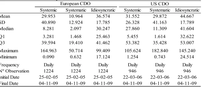
Figure 5 depicts the evolution of the European (Panel A) and US (Panel B) spreads. Before the subprime crisis, the CDO indexes and their tranches were mainly driven by the idiosyncratic component, the systemic and systematic spreads remaining almost negligible. At the beginning of the crisis, the systemic spreads increase substantially, achieving the first peak during the Bearn Stearns’ episode (see Appendix A1), in which the systemic spreads are higher than the idiosyncratic spreads in both economic areas. Up to the Lehman Brothers episode, the European and US spreads behaved similarly. After that episode, the European and US spreads behaved in a different way. From the Lehman episode to March 2009, in Europe, the systemic spread captures half of the iTraxx IG 5y’s32 behavior, whereas in the US, the systematic spread explains a higher proportion of the CDX IG 5y. Since March 2009, the idiosyncratic spread has explained most of the iTraxx IG 5y while in the US it has remained at the same level.33 Table 4 contains the descriptive statistics for the three spreads. In both economic areas, we observe that, on average, the higher spread is related to the idiosyncratic component followed by the systemic and systematic components.
e. Multivariate density
Another set of measures assesses the systemic risk through recovering the multivariate density of the analyzed portfolio. Within this line, we follow Segoviano et al. (2009), who propose a set of banking stability measures based on distress dependence, which is estimated by the Banking System Multivariate Density (BSMD).34 BSMD is the key element for measuring banking stability and is estimated by means of Consistent
32 Note that by construction, the idiosyncratic, systematic and systemic spreads add up the CDO index spreads.
33 At the end of the sample period, three jumps appear on the US spreads, corresponding to periods in which
out-the-roll series are employed (see Section 3).
34 The authors propose three different categories of measures: (a) common distress in the banks of the system;
Information Multivariate Density Optimizing (CIMDO) methodology (see Segoviano, 2006). CIMDO methodology is characterized by the CIMDO-copula function, which is able to capture both linear and non-linear distress dependences and allows changes throughout the economic cycle.35 Once the BSMD is recovered, the authors propose two measures for common distress in the banking system: the Joint Probability of Distress (JPoD) and the Banking Stability Index (BSI).
The estimation of the BSMD becomes harder as we increase the number of banks under analysis. In order to overcome this problem, we analyze this measure using “reduced portfolios” according to three criteria: (a) level of CDS spread; (b) level of liabilities; (c) level of the liabilities over market value ratio. For each period of time, we choose the three banks which are at the top of each classification and estimate the corresponding BSMD. Estimating the systemic risk measures over the “reduced portfolio” instead of over the whole portfolio is an approximation. However, we believe that the “reduced portfolios” could appropriately measure the systemic risk of the European and US banking systems because these categories (i.e., level of CDS spread; level of liabilities; level of the liabilities over market value ratio) usually give reliable indications about the soundness of the bank’s financial position.
The procedure for estimating these measures could be divided into two steps. The first one consists of recovering the BSMD by means of CIMDO-copula while the second one concerns the estimation of the common distress measures.
To recover the BSMD, we use the CIMDO-methodology. With this approach, a posterior multivariate distribution “p” (i.e., the CIMDO density) is obtained by using an optimization procedure by which a prior density “q” is updated with empirical information via a set of constraints based on the probability of defaults. According to the CIMDO density, the
35 By means of CIMDO-copula, the authors overcome the drawbacks of the characterization of distress
dependence of financial returns with correlations, which has been one of the most popular approaches for measuring systemic risk.
BSMD is the posterior density that is the closest to the prior distribution and that is consistent with the empirically estimated PoDs of the banks making up the “reduced portfolios”.
The optimal solution is represented by the following posterior multivariate density: ⎭ ⎬⎫ ⎩ ⎨⎧−⎢⎣⎡ + + + + ⎥⎦⎤ =
μ
λ
χ
∞λ
χ
∞λ
χ
∞ ) , [ 3 ) , [ 2 ) , [ 1ˆ
ˆ
ˆ
ˆ
1 exp ) , , ( ) , , ( ˆ z d y d x d x x x z y x q z y x p (14)where q(x,y,z) and p(x,y,z) are the prior and posterior multivariate distributions andχ is an
indicator variable which takes 1 in the defined interval and zero otherwise.36
This methodology takes the structural approach (Merton 1973) as the departing point. Assuming that its basic premises and economic intuition are correct, the initial hypothesis is that the portfolio follows a multivariate distribution, ( , , )∈ℜ3
z y x
q , which is a Normal
distribution N(0,I)where I is the identity matrix.
To recover the Lagrange multipliers (i.e.,μˆ,λˆ1,λˆ2,λˆ3), we solve the next system of equations
of each period of time:
∫ ∫ ∫
∫ ∫ ∫
∫ ∫ ∫
∫ ∫ ∫
∞ ∞ − ∞ ∞ − ∞ ∞ − ∞ ∞ ∞ − ∞ ∞ − ∞ ∞ − ∞ ∞ ∞ − ∞ ∞ − ∞ ∞ − ∞ = = = = 1 ) , , ( ˆ ) , , ( ˆ ) , , ( ˆ ) , , ( ˆ dxdydz z y x p PoD dxdydz z y x p PoD dxdydz z y x p PoD dxdydz z y x p z d y d x d x z t x y t x x t (15) where i tPoD refers to the probability of default of each individual bank (among the three
selected) at period t. The intuition is that the BSMD must satisfy the observed default probabilities for each bank.
36 x
mi is the default threshold which is defined as
(
i)
m i
d PoD
x =Φ−11−
where PoDmi is the average of the PoD for the previous 6 months and Φ−1stands for the inverse of the standard
Once we get the Lagrange multipliers on the basis of Equation (15), the BSMD is easily recovered by plugging the estimated Lagrange multipliers (i.e.μˆ,λˆ1,λˆ2,λˆ3) into Equation
(14). We repeat this process for each period and portfolio to obtain the BSMD of each portfolio over time.
After that, we estimate the two measures of common distress:
Joint Probability of Default (JPoD): This measure represents the probability of all banks
in the portfolio (i.e., the three selected banks) becoming distressed. The JPoD not only contains changes in the individual banks’ PoD but also captures changes in the distress dependence among banks, which increases in times of distress. This measure is defined as:
p x y z dxdydz JPoD z d y d x d x x x =
∫ ∫ ∫
∞ ∞ ∞ ) , , ( ˆ (16)Figure 6 shows the evolution of the JPD for European and US reduced portfolios. Up to the start of the subprime crisis, the JPD was almost zero. However, in the crisis period, there is a substantial increment of this risk. As can be seen in Panel A of Table 5, in both cases, the “reduced portfolio” that has higher risk is the one associated with the spread. On average, the spread portfolio’s JPD is 0.53 and 1.93 b.p. for the European and US portfolios, respectively. Regarding the liabilities and ratio portfolios, these averages are around 0.11 and 0.14 for Europe and 0.44 and 0.98 for US portfolios, respectively. The reason the spread portfolio displays a higher level of risk could be related to the close relationship that CDSs and systemic risk have maintained throughout the crisis. Three periods of stronger distress can be seen in Figure 6: March and October 2008 and March 2009. Our results are consistent to the ones of Segoviano et al. (2009) during the comparable period, although in our case, the probabilities are lower than theirs.
Banking Stability Index (BSI): This measure represents the expected number of banks to
become distressed, conditioned on the fact that at least one bank has become distressed. Hence, the higher this number is, the higher the instability. This measure is defined as:
) , , ( 1 ) ( ) ( ) ( z d y d x d z d y d x d x Z x Y x X P x Z P x Y P x X P BSI < < < − ≥ + ≥ + ≥ = (17)
This measure is an index which takes values between 1 and 3 due to the number of components in a “reduced portfolio”. The value 1 refers to the situation in which the stress in one institution causes no effect on the others. As can be seen in Figure 7, up to July 2007, this measure is almost 1. After that point, the distress between institutions is intensified. Panel B of Table 5 reports the descriptive statistics. There we observe that as in the JPD, the “CDS reduced portfolio” shows higher levels of stress. Our results are again in line with the findings of Segoviano et al. (2009).
f. “Co-risk management” measures
Our last set of systemic risk measures are based on the traditional risk management tools like Value-at-Risk (VaR) and Expected Shortfall (ES). Adrian et al. (2009) propose
estimating institution i’s Co-Value-at-Risk (CoVaRi) as the whole system (i.e., portfolio)’s VaRs conditioned on institution i being in distress (i.e., being at its unconditional VaRi
level). On the basis of CoVaR, they calculate the marginal contribution of institution i to the
overall systemic risk as the difference between CoVaR and the unconditional whole
system’s VaR, which is denoted asΔCoVaRi. Therefore, ΔCoVaRiallows us to determine how much an institution adds to overall systemic risk. Additionally, the authors argue that their methodology can be easily extended to other risk management tools like ES. The
Expected Shortfall is the basis of the systemic risk measure proposed by Acharya et al. (2010a). They propose a taxation system which is determined by the financial firm’s ES
a tool for monitoring the evolution of the level of the systemic risk in the system (i.e., portfolio) on a daily or weekly basis, and hence, we base our analysis on the “co-risk management” measures of Adrian et al. (2009).
Adrian et al. (2009) based their analysis on the growth rates of the market value of total financial assets ( i
t
X ), which are defined as:
i t i t i t i t i t i t i t LEV ME LEV ME LEV ME X 1 1 1 1 − − − − ⋅ ⋅ − ⋅ = (18) where i t
ME denotes the market value of institution i and LEVti is the ratio of total assets to
book equity. In order to estimate this growth rate for the whole portfolio, we calculate the total market weighted sum of the i
t
X across all institutions, which is:
i t i j j t j t i t i t portfolio t X LEV ME LEV ME X
∑ ∑
− − − − ⋅ ⋅ = 1 1 1 1 (19)VaR and CoVaR are estimated by means of quantile regression (Koenker and Bassett, 1978).
The time-variant measures are based on the following system of equations:
i portfolio t i t i portfolio t i portfolio i portfolio portfolio t portfolio t t portfolio portfolio portfolio t i t t i i i t X M X M X M X | | 1 | | 1 1 ε γ β α ε β α ε β α + + + = + + = + + = − − − (20) where i t
M is a set of state variables. Due to the fact that we are considering two different
portfolios (European and US), we employ two sets of state variables. The European one is composed of VDAX, the LIBOR-OIS referring to the Eurozone (see Section 4.b), the change in 3-month term Treasury Eurozone bill37, the difference between 10-year and 3-month Treasury rates, the difference between a BBB-rated 10-year bond and 10-year Treasury rates and the banking index return38 of European banks. For the US portfolio, we
37 See Section 3 for a detailed description.
38 Banking Indexes are return indexes which represent the theoretical aggregate growth in value of the
use VIX, the LIBOR-OIS of the US, the change in the 3-month Treasury bill, the difference between 10-year and 3-month Treasury rates, the difference between a BAA- rated 10-year bond and 10-year Treasury rates and the banking index return of US banks. In order to perform the quantile regression, we assume a confidence level of 5% (i.e.,α =0.05). This is like estimating a VaR at 5%.
Once the coefficients of Equation (21) have been estimated through quantile regression,
VaRs and CoVaR are estimated as follows:
i t i portfolio t i portfolio i portfolio i t t portfolio portfolio portfolio t t i i i t VaR M CoVaR M VaR M VaR | 1 | | 1 1 ˆ ˆ ˆ ˆ ˆ ˆ ˆ γ β α β α β α + + = + = + = − − − (21)
Subsequently, the marginal contribution of institution i to the overall systemic risk, which is
called Delta Co-Value-at-Risk (ΔCoVaRi), is calculated as the difference between CoVaRi
and the unconditional VaR of the whole system,
portfolio t i t i CoVaR VaR CoVaR= − Δ (22)
This measure allows us to determine how much systemic risk is associated with each bank in the portfolio. In order to obtain a global measure (up to now this systemic risk measure has been associated with each institution) to monitor the level of systemic risk in the whole portfolio, we aggregate the ΔCoVaRiof each bank, using two different criteria: first, equally
weighted, and second, using weights proportional to market capitalization.
Figure 8 shows the evolution of theΔCoVaRifor the European (Panel A) and US (Panel B)
portfolios. As is also the case with other systemic measures, both measures remain almost flat up to July 2007. Then, we distinguish three periods: the beginning of the crisis, which is characterized by the Bearn Stearns episode and presents a moderate increase in ΔCoVaRi as well as in its volatility; the Lehman Brothers episode, which generates the highest level of
distress in both portfolios; and the post-Lehman Brother bankruptcy, in which i
CoVaR
Δ goes down to a level similar to the one at the beginning of 2008.
Panel A of Table 6 reports the descriptive statistics of these measures. Within each economic area, two measures are estimated: equally weighted and weighted by market capitalization. In both portfolios, the former measure presents higher ΔCoVaRiand is more volatile. However, within the European portfolio, the measures are closer than within the US portfolio.
Additionally, we apply the “co-risk” methodology to the ES through the quantile regression.
The ES might provide additional insights with respect to the VaR due to the fact that the VaR is not a coherent measure (Artzner, Delbaen, Eber and Heath (1999)). Figure 9 shows
the evolution of theΔCoESi. Panel A refers to the European portfolio and Panel B to the US portfolio. Their behavior is similar to the behavior observed for theΔCoVaRi. Panel B of
Table 6 reports their descriptive statistics. We observe that, on average, the US weighted average measure of ΔCoESiis bigger than the European one.
Moreover, under both co-risk measures, we may observe that equally weighted systemic risk measures suggest higher systemic risk levels than the ones weighted by market capitalization. In the latter case, the results suggest that the largest banks (i.e., the banks with the highest market capitalization) are not necessarily the ones which generate the most systemic risk (see Table 6).
5. Comparing Measures
In this section, we choose the more informative variables within each group, regressing the measures against the influential events that have marked the main episodes of the crisis. Then we establish a common metric to be able to compare all of them. The common metric is achieved by standardizing the different systemic risk measures. Finally, we run a “horse
race” to rank the systemic risk measures according to their performance in a causality test, price discovery and McFadden R-squared.
a. Choosing measures in each group
Up to now several measures have been proposed within each group. However, most of them may provide redundant information. In this subsection, we choose the variables that provide more information within each group and economic area.
To choose the most informative variables about systemic risk we use of an influential events variable. This variable is a dummy which reflects most important adverse news during the financial crisis.39 Then we run logistic regressions, using each systemic risk measure as an explanatory variable, and choose the systemic risk measures with the highest McFadden R-squared.
Given that the frequency of the measures differs, we construct two influential events variables on both a daily and weekly basis. The former is a dummy variable that equals 1 on the event day as well as on the days before and after and is equal to zero otherwise. The other one is a categorical variable that ranges between 0 and 3, which represents the number of events within the corresponding week (i.e., number 3 captures three or more events while 0, 1 and 2 capture the corresponding number of events).
Regarding the daily measures (i.e., Principal Component Analysis, Libor spreads, CDO indexes and their tranches, multivariate density copulas and “co-risk management” tools), we run logit regressions, while for the weekly measure (i.e., structural models), we make use of multinomial logit regressions. In this framework, there is not any R-squared equivalent to the one of Ordinary Least Squared (OLS) (Long, 1997). However, to evaluate the goodness-of-fit for a logistic model, pseudo R-squared has been developed. Higher values of pseudo R-squared indicate better model fitting, although they cannot be
interpreted as in OLS squared. Our selection criterion is based on the McFadden R-squared40 because it has appropriate statistical properties.
For each group of measures, we run several logistic regressions in which the independent variable is lagged up to 14 days and 2 weeks, respectively.41 After that, we compute the average R-squared for each variable. Finally, we choose those variables that provide better average fit within each group and economic area.
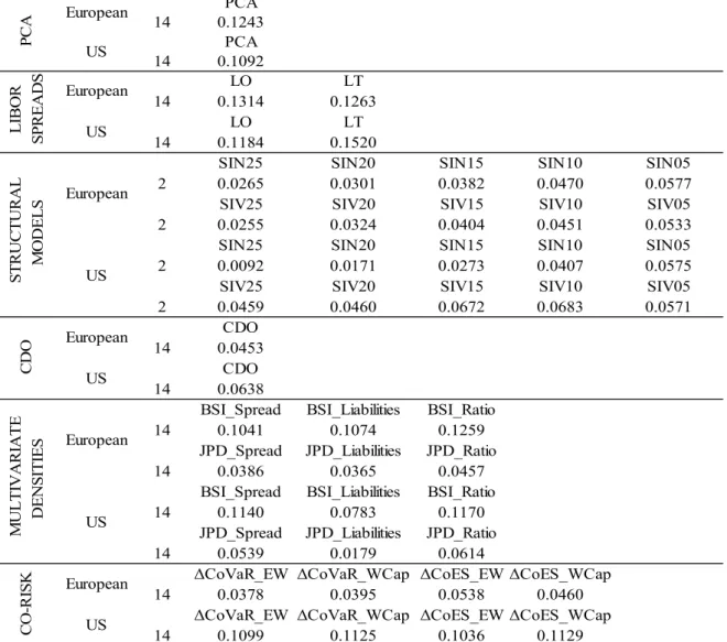
Table 7 summarizes the average McFadden R-squared. The degree of fit provided by the systemic risk measures is not very high. The highest for Europe (US) is LO (LT) with R-squared of 13% (15%).42Structural models and “co-risk management” tools do not give particularly good results, especially in Europe, with R-squared ranging from 1% to 10%. In these groups, the selected variables are the SIN05 (SIV10) and ΔCoES (ΔCoESand
CoVaR
Δ )43 in Europe (US). Similar fits are provided by the CDO-based measure in both economic areas. Regarding multivariate density variables, BSI whose “reduced portfolio” is based on the liabilities over market value ratio (BSI) usually has the best fit.
b. Horse race
In this subsection, we rank the selected variables across groups within each economic area. Firstly, we compare the evolution of the selected measures by portfolios. In order to carry out a comprehensive comparison, we establish a common metric. As Nardo, Saisana, Saltelli and Tarantola (2005) detail, there are several procedures for determining a common
40 McFadden R-squared is calculated as:
) ( ˆ ln ) ( ˆ ln 1 2 Intercept Full L L M L R = −
where MFull refers to the full model and MIntercept to the model without predictors. Lˆis the estimated likelihood. 41 Results do not change substantially when other lags are considered.
42 In order to construct LIBOR-TBILL in Europe, we
employ a “hypothetical” Treasury yield, which is the
weighted average of the Treasury yield of Eurozone members. The consequence of the lack of a European Treasury bill is that the LIBOR-TBILL does not capture the fact that in time of stress, Treasuries become especially valuable. On the contrary, LIBOR-TBILL provides more information in the US market, in which the tight relationship between bad news and Treasury bills becomes apparent.
metric.44 However, due to the nature of our dataset, we standardize all measures so as to get a comparable measure. Once we have standardized the variables, we rank the systemic risk measures within each economic area according to three criteria: (i) causality test; (ii) price discovery analysis; (iii) McFadden R-squared.
Panel A of Figure 10 depicts the evolution of the standardized European variables since 2007. From the beginning of the period up to the start of the subprime crisis, no variable gives signal of an increase in systemic risk, remaining flat up to that date. During the crisis, the PCA variable, BSI and CDO behave similarly, although the last measure achieves its maximum just before the Lehman Brothers episode while the other two measures get it during that episode. Regarding the variable SIN05, we have transformed the original weekly variable into a daily variable to make the comparison easier.45 This measure does not show any change up to April 2008. The measure LO shows the quickest reaction after the start of the subprime crisis. Finally, the ΔCoES measure is very volatile. Just before the Lehman
Brothers bankruptcy (see Appendix A1), it sharply increased, staying at high levels up to December 2008.
Panel B of Figure 10 depicts the standardized US systemic risk measures. We rule out the pre-crisis period as well as the ΔCoVaR in order to have a clearer picture during the crisis
period.46 In this figure, we can see that apart from LT measure, the European and US systemic risk measures (Principal Component Analysis, structural credit risk model, CDO indexes and their tranches, multivariate densities and “co-risk” management measures) perform very similar in both portfolios. Regarding LT, it seems to be a leading indicator at the beginning of the crisis. Moreover, after the Lehman Brothers episode, this measure
dramatically drops, finishing the sample period at levels similar to the pre-crisis period.
44 In the context of computing composite indicators among countries, they propose the following strategies:
ranking indicators, standardization, re-scaling and distance to the reference country, among others.
45 We use the same value for each week.
46 In this subsection, we show that according to our three classifications,ΔCoEStakes a better position in the
The first result that we find is the lack of early indicators (measures that warn about systemic risk before the hit takes place). Apart from LT and ΔCoES in the US (although the
second case is less clear), no measure could be employed as an early indicator. This fact is especially serious in certain measures like the ones which are based on structural models.47 The second characteristic that we find is that Libor Spreads are useful (mainly LT) while they are not subject to economic policies. Once they become a political-economic tool, their behavior is misleading and they do not appropriately measure the pressures of the financial system.
Once we have compared the standardized variables, we rank the systemic risk measures within each economic area.
i.
Causality test
The first classification is based on the Granger causality test (Granger, 1969). This test intuitively examines whether past changes in one variable, Xt, help to explain current
changes in another variable, Yt. If not, we conclude that Yt does not Grange cause Xt.
Formally, the Granger causality test was based on the follow regression:
p t i i t yi p i i t xi t X Y X α
∑
β∑
β ε = − = − + Δ + Δ + = Δ 1 1 (23) where Δ is the first-difference operator and ΔXand ΔYare stationary variables. We rejectthe null hypothesis that states Yt does not Granger cause to Xt if the coefficients βyi are jointly significant based on the standard F-test.
We perform the Granger causality test by pairs of measures within each economic area. The number of lags is determined on the basis of the Schwarz information criterion on the corresponding Vector Autoregressive (VAR) equation. In order to perform this analysis, we
47 We have estimated the probability that 5% of all banks considered go bankrupt for the next six months
restrict the sample from January 2007 to the end of the sample period. We get the same results using both the standardized and non-standardized systemic risk measures.
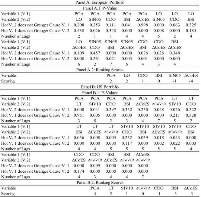
Table 8 summarizes the p-values for each test as well as the number of lags employed in the test and the corresponding ranking score, which is based on the p-values at a confidence level of 1%; Table 11 contains the aggregated ranking scores for the horse race. Panel A of Table 8 refers to the European portfolio measures. To rank the measures, we give a score of +1 to measure X if X causes another measure Y and we give a score of -1 to measure X if X is caused by Y. The best measure gets the highest positive score and the worst measure the highest negative score. For instance, PCA causes BSI and ΔCoES but it is not caused by any
other measure. Hence, PCA gets a final score of +2. LO gets a final score of +2, CDO scores +1, BSI scores par for the course, SIN5 scores -1 and, finally, ΔCoESscores -4.48
Therefore, the best measures in this account are PCA and LO and the worst measure isΔCoES . Panel B shows the results of the US portfolio. Applying the same procedure as
above, PCA scores +4, LT +2, SIV10 +1, ΔCoVaR scores par for the course, CDO -1 and,
finally, ΔCoESand BSI both score -3.49 Therefore, PCA is again the best measure and the
worst measures are BSI andΔCoES .
ii.
Price Discovery
The second classification is based on the Gonzalo and Granger’s (1995) price discovery methodology. This analysis allows us to determine, by pairs of measures, which measures reveal information more efficiently to the market. Formally, this price discovery methodology is based on the following VECM specification:
t i t p i i t t X X X =αβ′ + Γ +ε Δ − = −
∑
1 1 (24)48 We observe that PCA, LO, CDO and BSI Granger cause at least two systemic risk measures while ΔCoES
is Granger caused by all the measures considered.
49 We observe that PCA, LT, SIV10 and CDO measures Granger-cause other systemic risk measures while
CoES