A Line-Search Algorithm Inspired by the Adaptive Cubic
Regularization Framework and Complexity Analysis
E. Bergou ∗ Y. Diouane† S. Gratton‡ May 30, 2018
Abstract
Adaptive regularized framework using cubics has emerged as an alternative to line-search and trust-region algorithms for smooth nonconvex optimization, with an optimal complexity amongst second-order methods. In this paper, we propose and analyze the use of an iter-ation dependent scaled norm in the adaptive regularized framework using cubics. Within such scaled norm, the obtained method behaves as a line-search algorithm along the quasi-Newton direction with a special backtracking strategy. Under appropriate assumptions, the new algorithm enjoys the same convergence and complexity properties as adaptive regular-ized algorithm using cubics. The complexity for finding an approximate first-order stationary point can be improved to be optimal whenever a second order version of the proposed algo-rithm is regarded. In a similar way, using the same scaled norm to define the trust-region neighborhood, we show that the trust-region algorithm behaves as a line-search algorithm. The good potential of the obtained algorithms is shown on a set of large scale optimization problems.
Keywords: Nonlinear optimization, unconstrained optimization, line-search methods, adaptive regularized framework using cubics, trust-region methods, worst-case complexity.
1
Introduction
An unconstrained nonlinear optimization problem considers the minimization of a scalar function known as the objective function. Classical iterative methods for solving the previous problem are trust-region (TR) [8, 20], line-search (LS) [10] and algorithms using cubic regularization. The latter class of algorithms has been first investigated by Griewank [15] and then by Nesterov and Polyak [18]. Recently, Cartis et al [5] proposed a generalization to an adaptive regularized framework using cubics (ARC).
The worst-case evaluation complexity of finding anǫ-approximate first-order critical point using TR or LS methods is shown to be computed in at most O(ǫ−2) objective function or gradient evaluations, where ǫ∈]0,1[ is a user-defined accuracy threshold on the gradient norm
∗MaIAGE, INRA, Universit´e Paris-Saclay, 78350 Jouy-en-Josas, France ([email protected]). †Institut Sup´erieur de l’A´eronautique et de l’Espace (ISAE-SUPAERO), Universit´e de Toulouse, 31055
Toulouse Cedex 4, France ([email protected]).
‡INP-ENSEEIHT, Universit´e de Toulouse, 31071 Toulouse Cedex 7, France (
[17, 14, 7]. Under appropriate assumptions, ARC takes at most O(ǫ−3/2) objective function or gradient evaluations to reduce the gradient of the objective function norm belowǫ, and thus it is improving substantially the worst-case complexity over the classical TR/LS methods [4]. Such complexity bound can be improved using higher order regularized models, we refer the reader for instance to the references [2, 6].
More recently, a non-standard TR method [9] is proposed with the same worst-case com-plexity bound as ARC. It is proved also that the same worst-case comcom-plexity O(ǫ−3/2) can be achieved by mean of a specific variable-norm in a TR method [16] or using quadratic regular-ization [3]. All previous approaches use a cubic sufficient descent condition instead of the more usual predicted-reduction based descent. Generally, they need to solve more than one linear system in sequence at each outer iteration (by outer iteration, we mean the sequence of the iterates generated by the algorithm), this makes the computational cost per iteration expensive. In [1], it has been shown how to use the so-called energy norm in the ARC/TR framework when a symmetric positive definite (SPD) approximation of the objective function Hessian is available. Within the energy norm, ARC/TR methods behave as LS algorithms along the Newton direction, with a special backtracking strategy and an acceptability condition in the spirit of ARC/TR methods. As far as the model of the objective function is convex, in [1] the proposed LS algorithm derived from ARC enjoys the same convergence and complexity analysis properties as ARC, in particular the first-order complexity bound ofO(ǫ−3/2). In the complexity analysis of ARC method [4], it is required that the Hessian approximation has to approximate accurately enough the true Hessian [4, Assumption AM.4], obtaining such convex approximation may be out of reach when handling nonconvex optimization. This paper generalizes the proposed methodology in [1] to handle nonconvex models. We propose to use, in the regularization term of the ARC cubic model, an iteration dependent scaled norm. In this case, ARC behaves as an LS algorithm with a worst-case evaluation complexity of finding anǫ-approximate first-order critical point of O(ǫ−2) function or gradient evaluations. Moreover, under appropriate assumptions, a second order version of the obtained LS algorithm is shown to have a worst-case complexity of O(ǫ−3/2).
The use of a scaled norm was first introduced in [8, Section 7.7.1] for TR methods where it was suggested to use the absolute-value of the Hessian matrix in the scaled norm, such choice was described as “the ideal trust region” that reflects the proper scaling of the underlying problem. For a large scale indefinite Hessian matrix, computing its absolute-value is certainly a computationally expensive task as it requires a spectral decomposition. This means that for large scale optimization problems the use of the absolute-value based norm can be seen as out of reach. Our approach in this paper is different as it allows the use of subspace methods.
In fact, as far as the quasi-Newton direction is not orthogonal with the gradient of the objective function at the current iterate, the specific choice of the scaled norm renders the ARC subproblem solution collinear with the quasi-Newton direction. Using subspace methods, we also consider the large-scale setting when the matrix factorizations are not affordable, implying that only iterative methods for computing a trial step can be used. Compared to the classical ARC, when using the Euclidean norm, the dominant computational cost regardless the function evaluation cost of the resulting algorithm is mainly the cost of solving a linear system for successful iterations. Moreover, the cost of the subproblem solution for unsuccessful iterations is getting inexpensive and requires only an update of a scalar. Hence, ARC behaves as an LS algorithm along the quasi-Newton direction, with a special backtracking strategy and an acceptance criteria in the sprite of ARC algorithm.
In this context, the obtained LS algorithm is globally convergent and requires a number of iterations of order ǫ−2 to produce an ǫ-approximate first-order critical point. A second order
version of the algorithm is also proposed, by making use of the exact Hessian or at least of a good approximation of the exact Hessian, to ensure an optimal worst-case complexity bound of order ǫ−3/2. In this case, we investigate how the complexity bound depends on the quality of the chosen quasi-Newton direction in terms of being a sufficient descent direction. In fact, the obtained complexity bound can be worse than it seems to be whenever the quasi-Newton direction is approximately orthogonal with the gradient of the objective function. Similarly to ARC, we show that the TR method behaves also as an LS algorithm using the same scaled norm as in ARC. Numerical illustrations over a test set of large scale optimization problems are given in order to assess the efficiency of the obtained LS algorithms.
The proposed analysis in this paper assumes that the quasi-Newton direction is not orthog-onal with the gradient of the objective function during the minimization process. When such assumption is violated, one can either modify the Hessian approximation using regularization techniques or, when a second order version of the LS algorithm is regarded, switch to the classi-cal ARC algorithm using the Euclidean norm until this assumption holds. In the latter scenario, we propose to check first if there exists an approximate quasi-Newton direction, among all the iterates generated using a subspace method, which is not orthogonal with the gradient and that satisfies the desired properties. If not, one minimizes the model using the Euclidean norm until a new successful outer iteration is found.
We organize this paper as follows. In Section 2, we introduce the ARC method using a general scaled norm and derive the obtained LS algorithm on the base of ARC when a specific scaled norm is used. Section 3 analyses the minimization of the cubic model and discusses the choice of the scaled norm that simplifies solving the ARC subproblem. Section 4 discusses first how the iteration dependent can be chosen uniformly equivalent to the Euclidean norm, and then we propose a second order LS algorithm that enjoys the optimal complexity bound. The section ends with a detailed complexity analysis of the obtained algorithm. Similarly to ARC and using the same scaled norm, an LS algorithm in the spirit of TR algorithm is proposed in Section 5. Numerical tests are illustrated and discussed in Section 6. Conclusions and future improvements are given in Section 7.
2
ARC Framework Using a Specific
M
k-Norm
2.1 ARC Framework
We consider a problem of unconstrained minimization of the form min
x∈Rnf(x), (1)
where the objective functionf :Rn→Ris assumed to be continuously differentiable. The ARC framework [5] can be described as follows: at a given iterate xk, we definemQk :Rn→R as an
approximate second-order Taylor approximation of the objective functionf aroundxk, i.e., mQk(s) = f(xk) +s⊤gk+
1 2s
⊤B
ks, (2)
where gk =∇f(xk) is the gradient off at the current iterate xk, and Bk is a symmetric local
approximates the global minimizer of the cubic modelmk(s) =mQk(s) +13σkksk3Mk, i.e.,
sk≈arg min
s∈Rnmk(s), (3)
wherek.kMk denotes an iteration dependent scaled norm of the formkxkMk = p
x⊤M
kxfor all x ∈Rn and Mk is a given SPD matrix. σk >0 is a dynamic positive parameter that might be
regarded as the reciprocal of the TR radius in TR algorithms (see [5]). The parameter σk is
taking into account the agreement between the objective function f and the model mk.
To decide whether the trial step is acceptable or not a ratio between the actual reduction and the predicted reduction is computed, as follows:
ρk =
f(xk)−f(xk+sk) f(xk)−mQk(sk)
. (4)
For a given scalar 0 < η < 1, the kth outer iteration will be said successful if ρk ≥ η, and
unsuccessful otherwise. For allsuccessful iterations we setxk+1 =xk+sk; otherwise the current
iterate is kept unchanged xk+1 = xk. We note that, unlike the original ARC [5, 4] where the
cubic model is used to evaluate the denominator in (4), in the nowadays works related to ARC, only the quadratic approximation mQk(sk) is used in the comparison with the actual value of f without the regularization parameter (see [2] for instance). Algorithm 1 gives a detailed description of ARC.
Algorithm 1: ARC algorithm.
Data: select an initial pointx0 and the constant 0< η <1. Set the initial
regularization σ0 >0 and σmin∈]0, σ0], set also the constants 0< ν1≤1< ν2. fork= 1,2, . . . do
Compute the stepsk as an approximate solution of (3) such that
mk(sk) ≤ mk(sck) (5)
wheresc
k=−δkcgk and δkc= arg mint>0 mk(−tgk) ;
if ρk ≥η then
Setxk+1 =xk+sk and σk+1 = max{ν1σk, σmin}; else
Setxk+1 =xk andσk+1=ν2σk;
end end
The Cauchy step sck, defined in Algorithm 1, is computationally inexpensive compared to the computational cost of the global minimizer of mk. The condition (5) on sk is sufficient for
ensuring global convergence of ARC to first-order critical points.
From now on, we will assume that first-order stationarity is not reached yet, meaning that the gradient of the objective function is non null at the current iteration k (i.e., gk 6= 0). Also,
k · k will denote the vector or matrix ℓ2-norm, sgn(α) the sign of a real α, and In the identity
2.2 An LS Algorithm Inspired by the ARC Framework
Using a specific Mk-norm in the definition of the cubic model mk, we will show that ARC
framework (Algorithm 1) behaves as an LS algorithm along the quasi-Newton direction. In a previous work [1], when the matrix Bk is assumed to be positive definite, we showed that
the minimizer sk of the cubic model defined in (3) is getting collinear with the quasi-Newton
direction when the matrixMkis set to be equal toBk. In this section we generalize our proposed
approach to cover the case where the linear systemBks=−gk admits an approximate solution
and Bk is not necessarily SPD.
Let sQk be an approximate solution of the linear system Bks= −gk and assume that such
step sQk is not orthogonal with the gradient of the objective function at xk, i.e., there exists
an ǫd >0 such that |g⊤ks Q
k| ≥ ǫdkgkkksQkk. Suppose that there exists an SPD matrix Mk such
that MksQk = βkksQkk 2 g⊤ ks Q k
gk where βk ∈]βmin, βmax[ and βmax > βmin > 0, in Theorem 4.1 we will
show that such matrix Mk exists. By using the associated Mk-norm in the definition of the
cubic model mk, one can show (see Theorem 3.3) that an approximate stationary point of the
subproblem (3) is of the form
sk = δksQk, where δk= 2 1−sgn(g⊤ ks Q k) r 1 + 4σkks Q kk 3 Mk |g⊤ ks Q k| . (6)
Forunsuccessful iterations in Algorithm 1, since the step direction sQk does not change, the approximate solution of the subproblem, given by (6), can be obtained only by updating the step-size δk. This means that the subproblem computational cost of unsuccessful iterations
is getting straightforward compared to solving the subproblem as required by ARC when the Euclidean norm is used (see e.g., [5]). As a consequence, the use of the proposed Mk-norm in
Algorithm 1 will lead to a new formulation of ARC algorithm where the dominant computational cost, regardless the objective function evaluation cost, is the cost of solving a linear system for successful iterations. In other words, with the proposed Mk-norm, the ARC algorithm behaves
as an LS method with a specific backtracking strategy and an acceptance criteria in the sprite of ARC algorithm, i.e., the step is of the formsk=δksQk where the step lengthδk >0 is chosen
such as
ρk=
f(xk)−f(xk+sk) f(xk)−mQk(sk)
≥η and mk(sk)≤mk(−δckgk). (7)
The step lengths δk and δkc are computed respectively as follows: δk = 2 1−sgn(g⊤ ks Q k) r 1 + 4σkβ 3/2 k ks Q kk 3 |g⊤ ks Q k| , (8) and δkc = 2 g⊤ kBkgk kgkk2 + r g⊤ kBkgk kgkk2 2 + 4σkχ3k/2kgkk (9)
where χk =βk 5 2 −32cos(̟k)2+ 2 1−cos(̟k)2 cos(̟k) 2 and cos(̟k) = g ⊤ ks Q k kgkkksQkk . The Mk-norms of
the vectorssQk andgkin the computation ofδkandδkchave been substituted using the expressions
given in Theorem 4.1. The value of σk is set equal to the current value of the regularization
parameter as in the original ARC algorithm. For large values of δk the decrease condition (7)
may not be satisfied. In this case, the value of σk is enlarged using an expansion factor ν2 >1.
Iteratively, the value of δk is updated and the acceptance condition (7) is checked again, until
its satisfaction.
We referred the ARC algorithm, when the proposed scaledMk-norm is used, by LS-ARC as
it behaves as an LS type method in this case. Algorithm 2 details the final algorithm. We recall again that this algorithm is nothing but ARC algorithm using a specificMk-norm.
Algorithm 2: LS-ARC algorithm.
Data: select an initial pointx0 and the constants 0< η <1, 0< ǫd<1,
0< ν1 ≤1< ν2 and 0< βmin< βmax. Set σ0>0 and σmin ∈]0, σ0]. fork= 1,2, . . . do
Choose a parameter βk∈]βmin, βmax[;
LetsQk be an approximate solution ofBks=−gk such as |g⊤ks Q
k| ≥ǫdkgkkksQkk ;
Setδk and δkc respectively using (8) and (9);
while condition (7) is not satisfied do
Setσk ←ν2σk and update δk and δkc respectively using (8) and (9);
end
Setsk=δksQk,xk+1=xk+sk and σk+1= max{ν1σk, σmin}; end
Note that in Algorithm 2 the stepsQk may not exist or be approximately orthogonal with the gradientgk. A possible way to overcome this issue can be ensured by modifying the matrixBk
using regularization techniques. In fact, as far as the Hessian approximation is still uniformly bounded from above, the global convergence will still hold as well as a complexity bound of order ǫ−2 to drive the norm of the gradient belowǫ∈]0,1[ (see [5] for instance).
The complexity bound can be improved to be of the order ofǫ−3/2 if a second order version
of the algorithm LS-ARC is used, by making Bk equals to the exact Hessian or at least being
a good approximation of the exact Hessian (as in Assumption 4.2 of Section 4). In this case, modify the matrix Bk using regularization techniques such that the step sQk approximates the linear system Bks= −gk and |gk⊤sQk| ≥ ǫdkgkkksQkk is not trivial anymore. This second order
version of the algorithm LS-ARC will be discussed in details in Section 4 where convergence and complexity analysis, when the proposed Mk-norm is used, will be outlined.
3
On the Cubic Model Minimization
In this section, we assume that the linear system Bks = −gk has a solution. We will mostly
focus on the solution of the subproblem (3) for a given outer iteration k. In particular, we will explicit the condition to impose on the matrix Mk in order to get the solution of the ARC
subproblem collinear with the stepsQk. Hence, in such case, one can get the solution of the ARC subproblem at a modest computational cost.
The step sQk can be obtained exactly using a direct method if the matrix Bk is not too
large. Typically, one can use the LDLT factorization to solve this linear system. For large
scale optimization problems, computingsQk can be prohibitively computationally expensive. We will show that it will be possible to relax this requirement by letting the step sQk be only an approximation of the exact solution using subspace methods.
In fact, when an approximate solution is used and as far as the global convergence of Al-gorithm 1 is concerned, all what is needed is that the solution of the subproblem (3) yields a decrease in the cubic model which is as good as the Cauchy decrease (as emphasized in condition (5)). In practice, a version of Algorithm 2 solely based on the Cauchy step would suffer from the same drawbacks as the steepest descent algorithm on ill-conditioned problems and faster convergence can be expected if the matrix Bk influences also the minimization direction. The
main idea consists of achieving a further decrease on the cubic model, better than the Cauchy decrease, by projection onto a sequence of embedded Krylov subspaces. We now show how to use a similar idea to compute a solution of the subproblem that is computationally cheap and yields the global convergence of Algorithm 2.
A classical way to approximate the exact solutionsQk is by using subspace methods, typically a Krylov subspace method. For that, let Lk be a subspace of Rn and l its dimension. Let Qk
denotes an n×l matrix whose columns form a basis of Lk. Thus for all s ∈ Lk, we have sk =Qkzk, for somezk ∈Rl. In this case, sQk denotes the exact stationary point of the model
functionmQ over the subspaceL
k when it exists.
For both cases, exact and inexact, we will assume that the stepsQk is not orthogonal with the gradient gk. In what comes next, we state our assumption onsQk formally as follows:
Assumption 3.1 The model mQk admits a stationary point sQk such as |gk⊤sQk| ≥ ǫdkgkkksQkk
where ǫd>0 is a pre-defined positive constant.
We define also a Newton-like step sN
k associated with the minimization of the cubic model mk over the subspace Lk on the following way, when sQk corresponds to the exact solution of Bks=−gk by
sNk =δkNsQk, where δkN= arg min
δ∈Ik
mk(δsQk), (10)
where Ik = R+ if gk⊤s Q
k < 0 and Ik = R− otherwise. If sQk is computed using an iterative
subspace method, then sNk =QkzkN,wherezNk is the Newton-like step , as in (10), associated to
the following reduced subproblem: min z∈Rlf(xk) +z ⊤Q⊤ kgk+ 1 2z ⊤Q⊤ kBkQkz+ 1 3σkkzk 3 Q⊤ kMkQk. (11)
Theorem 3.1 Let Assumption 3.1 hold. The Newton-like step sNk is of the form
sNk =δNksQk, where δNk = 2 1−sgn(g⊤ ks Q k) r 1 + 4σkks Q kk 3 Mk |g⊤ ks Q k| . (12)
Proof. Consider first the case where the step sQk is computed exactly (i.e., BksQk = −gk). In
this case, for all δ ∈ Ik, one has
mk(δsQk)−mk(0) = δg⊤ksQk + δ2 2[s Q k]⊤Bk[sQk] + σ|δ|3 3 ks Q kk3Mk = (gk⊤sQk)δ−(gk⊤sQk)δ 2 2 + (σkks Q kk3Mk) |δ|3 3 . (13) If g⊤ ks Q
k < 0 (hence, Ik = R+), we compute the value of the parameter δkN at which the
unique minimizer of the above function is attained. Taking the derivative of (13) with respect to δ and equating the result to zero, one gets
0 = g⊤ksQk −(gk⊤sQk)δNk +σkksQkk3Mk δ
N
k
2
, (14)
and thus, since δN
k >0, δkN = gk⊤sQk + r g⊤ ks Q k 2 −4σk(g⊤kskQ)ksQkk3Mk 2σkksQkk3Mk = 2 1 + r 1−4σkks Q kk 3 Mk g⊤ ks Q k .
Ifgk⊤sQk > 0 (hence, Ik =R−),and again by taking the derivative of (13) with respect to δ and equating the result to zero, one gets
0 = g⊤ksQk −(gk⊤sQk)δNk −σkksQkk3Mk δ
N
k
2
, (15)
and thus, since δNk <0 in this case,
δkN = gk⊤sQk + r g⊤ksQk2+ 4σk(g⊤ks Q k)ks Q kk3Mk 2σkksQkk3Mk = 2 1− r 1 + 4σkks Q kk 3 Mk g⊤ ks Q k .
From both cases, one deduces that δkN= 2
1−sgn(g⊤ ks Q k) v u u t1+4 σkksQkk3 Mk |gk⊤sQk| .
Consider now the case where sQk is computed using an iterative subspace method. In this cas, one hassNk =QkzkN, wherezkNis the Newton-like step associated to the reduced subproblem
(11). Hence by applying the first part of the proof (the exact case) to the reduced subproblem (11), it follows that zkN= ¯δkNzQk where ¯δNk = 2 1−sgn((Q⊤ kgk)⊤z Q k) s 1 + 4 σkkzkQk 3 Q⊤kMkQk |(Q⊤ kgk)⊤zQk| ,
substitutingzkNin the formula sNk =QkzNk, one gets sNk = Qk 2 1−sgn((Q⊤ kgk)⊤zkQ) s 1 + 4 σkkzkQk 3 Q⊤kMkQk |Q⊤ kgk)⊤zkQ| zkQ = 2 1−sgn(g⊤ kQkz Q k) r 1 + 4σkkQkz Q kk 3 Mk |g⊤ kQkzkQ| QkzkQ = 2 1−sgn(gk⊤sQk) r 1 + 4σkks Q kk 3 Mk |g⊤ ks Q k| sQk.
In general, for ARC algorithm, the matrixMk can be any arbitrary SPD matrix. Our goal,
in this section, is to determine how one can choose the matrix Mk so that the Newton-like step sNk becomes a stationary point of the subproblem (3). The following theorem gives explicitly the necessary and sufficient condition on the matrix Mk to reach this aim.
Theorem 3.2 Let Assumption 3.1 hold. The step sNk is a stationary point for the subproblem (3) if and only if there exists θk>0 such thatMksQk = g⊤θk
ks Q k
gk. Note that θk =ksQkk2Mk.
Proof. Indeed, in the exact case, if we suppose that the step sN
k is a stationary point of the
subproblem (3), this means that
∇mk(sNk) = gk+BksNk +σkksNkkMkMks N k = 0, (16) In another hand, sN k =δkNs Q k where δkN is solution of g⊤ks Q k −(gk⊤s Q k)δkN+σkks Q kk3Mk|δ N k|δkN = 0
(such equation can be deduced from (14) and (15)). Hence, we obtain that 0 = ∇mk(sNk) =gk−δNkgk+σk|δkN|δNkksQkkMkMks Q k = 1−δNk gk+ σkksQkk3Mk g⊤ ks Q k |δkN|δkN ! g⊤ ks Q k ksQk2 Mk MksQk ! = σkks Q kk3Mk g⊤ ks Q k |δNk|δNk ! gk− g⊤ ks Q k ksQkk2 Mk MksQk ! .
Equivalently, we conclude thatMksQk = θk g⊤
ks Q k
gkwhereθk=ksQkk2Mk >0. A similar proof applies when a subspace method is used to compute sQk.
The key condition to ensure that the ARC subproblem stationary point is equal to the Newton-like step sNk, is the choice of the matrix Mk which satisfies the following secant-like
equationMksQk = θk g⊤
ks Q k
gkfor a givenθk>0. The existence of such matrixMkis not problematic
as far as Assumption 3.1 holds. In fact, Theorem 4.1 will explicit a range of θk >0 for which
computation of the Mk-norm of sQk. Therefore an explicit formula of the matrix Mk is not
needed, and only the value of θk=ksQkk2Mk suffices for the computations.
When the matrixMksatisfies the desired properties (as in Theorem 3.2), one is ensured that sN
k is a stationary point for the modelmk. However, ARC algorithm imposes on the approximate
step to satisfy the Cauchy decrease given by (5), and such condition is not guaranteed by sNk as the model mk may be non-convex. In the next theorem, we show that for a sufficiently large σk, sNk is getting the global minimizer of mk and thus satisfying the Cauchy decrease is not an
issue anymore.
Theorem 3.3 Let Assumption 3.1 hold. Let Mk be an SPD matrix which satisfies MksQk = θk
g⊤
ks Q k
gk for a fixed θk>0. If the matrix Q⊤k(Bk+σkksNkkMkMk)Qk is positive definite, then the
step sN
k is the unique minimizer of the subproblem (3) over the subspace Lk.
Proof. Indeed, when sQ is computed exactly (i.e., Q
k = In and Lk = Rn), then using [8,
Theorem 3.1] one has that, for a given vector s∗
k, it is a global minimizer of mk if and only if it
satisfies
(Bk+λ∗kMk)s∗k=−gk
whereBk+λ∗kMk is positive semi-definite matrix andλ∗k=σkks∗kkMk. Moreover, ifBk+λ∗kMk
is positive definite, s∗ k is unique. SinceMksQk = g⊤θk ks Q k
gk, by applying Theorem 3.2, we see that
(Bk+λNkMk)sNk =−gk
with λNk =σkksNkkMk. Thus, if we assume that Bk+λ
N
kMk is positive definite matrix, then sNk
is the unique global minimizer of the subproblem (3).
Consider now, the case wheresQk is computed using a subspace method, sinceMksQk = g⊤θk
ks Q k
gk
one has that Q⊤
kMkQkzkQ = (Q⊤θk
kgk)⊤zkQ
Q⊤
kgk. Hence, if we suppose that the matrix Q⊤k(Bk+ λNkMk)Qk is positive definite, by applying the same proof of the exact case to the reduced
subproblem (11), we see that the stepzN
k is the unique global minimizer of the subproblem (11).
We conclude that sNk =QkzkN is the global minimizer of the subproblem (3) over the subspace
Lk.
Theorem 3.3 states that the step sN
k is the global minimizer of the cubic model mk over
the subspace Lk as far as the matrix Q⊤k(Bk +σkksNkkMkMk)Qk is positive definite, where
λNk =σkksNkkMk. Note that λNk = σkksNkkMk = 2σkksQkkMk 1−sgn(g⊤ksQk) r 1 + 4σkks Q kk 3 Mk |g⊤ ks Q k| →+∞ asσk→ ∞.
Thus, since Mk is an SPD matrix and the regularization parameter σk is increased for
unsuc-cessful iterations in Algorithm 1, the positive definiteness of matrixQ⊤k(Bk+σkksNkkMkMk)Qkis guaranteed after finitely many unsuccessful iterations. In other words, one would have insurance that sN
4
Complexity Analysis of the LS-ARC Algorithm
For the well definiteness of the algorithm LS-ARC, one needs first to show that the proposedMk
-norm is uniformly equivalent to the Euclidean -norm. The next theorem gives a range of choices for the parameter θk to ensure the existence of an SPD matrixMk such asMksQk = g⊤θk
ks Q k
gk and
theMk-norm is uniformly equivalent to theℓ2-norm. Theorem 4.1 Let Assumption 3.1 hold. If
θk=βkksQkk2 where βk ∈]βmin, βmax[ and βmax> βmin>0, (17) then there exists an SPD matrix Mk such as
i) MksQk = g⊤θk
ks Q k
gk,
ii) the Mk-norm is uniformly equivalent to the ℓ2-norm on Rn and for all x∈Rn, one has
√ βmin √ 2 kxk ≤ kxkMk ≤ √ 2βmax ǫd k xk. (18)
iii) Moreover, one hasksQkk2Mk =βkksQkk2 andkgkk2Mk =χkkgkk
2whereχ k=βk 5 2 −32cos(̟k)2+ 2 1−cos(̟ cos(̟ andcos(̟k) = g ⊤ ks Q k kgkkksQkk Proof. Let ¯sQk = s Q k
ksQkk and ¯gk be an orthonormal vector to ¯s
Q k (i.e., k¯gkk = 1 and ¯g⊤ks¯ Q k = 0) such that gk kgkk = cos(̟k)¯sQk + sin(̟k) ¯gk. (19)
For a given θk=βkksQkk2 whereβk ∈]βmin, βmax[ and βmax> βmin >0,one would like to
construct an SPD matrixMk such as MksQk = gθ⊤kgk
ks Q k , hence Mk¯sQk = θkgk gk⊤sQkksQkk = θkkgkk g⊤ksQkksQkk cos(̟k)¯sQk + sin(̟k)¯gk = βks¯Qk +βktan(̟k)¯gk.
Using the symmetric structure of the matrixMk, letγk be a positive parameter such as Mk= h ¯ sQk,g¯k i Nk h ¯ sQk,¯gk i⊤ whereNk= βk βktan(̟k) βktan(̟k) γk .
The eigenvalues λmin
k and λmaxk of the matrix Nk are the roots of λ2−(βk+γk)λ+βkγk−(βktan(̟k))2 = 0,
hence λmink = (βk+γk)− √ ϑk 2 and λ max k = (βk+γk) +√ϑk 2 ,
whereϑk= (βk−γk)2+ 4 (βktan(̟k))2.Note that both eigenvalues are monotonically
increas-ing as functions of γk.
One may choose λmink to be equal to 12βk = 12ksθQk kk2
, therefore λmink > 12βmin is uniformly
bounded away from zero. In this case, from the expression of λmin
k , we deduce that γk = 2βktan(̟k)2+βk/2 and λmaxk = 3 4βk+βktan(̟k) 2+ r 1 16β 2 k+ 1 2β 2 ktan(̟k)2+βk2tan(̟k)4 = βk 3 4 + tan(̟k) 2+ r 1 16 + 1 2tan(̟k)2+ tan(̟k)4 ! = βk 1 + 2 tan(̟k)2 .
From Assumption 3.1, i.e.,|g⊤ksQk| ≥ǫdkgkkksQkkwhereǫd>0, one has tan(̟k)2 ≤ 1−ǫ 2 d ǫ2 d .Hence, λmaxk ≤βmax 1 + 21−ǫ 2 d ǫ2 d ≤ 2βǫmax2 d
A possible choice for the matrix Mk can be obtained by completing the vectors family{s¯Qk,¯gk}
to an orthonormal basis {s¯Qk,¯gk, q3, q4, . . . , qn}of Rn as follows: Mk= [¯sQk,g¯k, q3, . . . , qn] Nk 0 0 D [¯sQk,g¯k, q3, . . . , qn]⊤,
where D = diag(d3, . . . , dn) ∈ R(n−2)×(n−2) with positive diagonal entrees independent from k
. One concludes that for all θk =βkksQkk2 where βk ∈]βmin, βmax[ and βmax > βmin >0, the
eigenvalue of the constructed Mkare uniformly bounded away from zero and from above, hence
the scaled Mk-norm is uniformly equivalent to theℓ2-norm on Rn and for all x∈Rn, one has
√ βmin √ 2 kxk ≤ q λmink kxk ≤ kxkMk ≤ q λmaxk kxk ≤ √ 2βmax ǫd k xk. By multiplyingMksQk = g⊤θk ks Q k
gk from both sides bysQk, one gets
ksQkk2Mk =θk=βkksQkk2.
Moreover, using (19) and (20), one has kgkk2Mk = kgkk 2cos(̟ k)¯sQk + sin(̟k) ¯gk ⊤ cos(̟k)Mk¯skQ+ sin(̟k)Mkg¯k = kgkk2 θkcos(̟k)2 ksQkk2 +γksin(̟k) 2+ 2 sin(̟ k) cos(̟k) θktan(̟k)2 ksQkk2 ! = βkkgkk2 cos(̟k)2+ 5 2sin(̟k) 2+ 2 sin(̟ k)2tan(̟k)2 = βkkgkk2 5 2 − 3 2cos(̟k) 2+ 2 1−cos(̟k)2 cos(̟k) 2! .
A direct consequence of Theorem 4.1 is that, by choosingθk>0 of the formβkksQkk2 where βk ∈]βmin, βmax[ and βmax > βmin >0 during the application of LS-ARC algorithm, the global
convergence and complexity bounds of LS-ARC algorithm can be derived straightforwardly from the classical ARC analysis [4]. In fact, as far as the objective function f is continuously differentiable, its gradient is Lipschitz continuous, and its approximated Hessian Bk is bounded
for all iterations (see [4, Assumptions AF1, AF4, and AM1]), the LS-ARC algorithm is globally convergent and will required at most a number of iterations of order ǫ−2 to produce a pointxǫ
withk∇f(xǫ)k ≤ǫ[4, Corollary 3.4].
In what comes next, we assume the following on the objective functionf:
Assumption 4.1 Assume that f is twice continuously differentiable with Lipschitz continuous Hessian, i.e., there exists a constant L≥0 such that for all x, y∈Rn one has
k∇2f(x)− ∇2f(y)k ≤Lkx−yk.
When the matrixBkis set to be equal to the exact Hessian of the problem and under Assumption
4.1, one can improve the function-evaluation complexity to be O(ǫ−3/2) for ARC algorithm by imposing, in addition to the Cauchy decrease, another termination condition during the computation of the trial step sk (see [4, 2]). Such condition is of the form
k∇mk(sk)k ≤ ζkskk2, (20)
where ζ >0 is a given constant chosen at the start of the algorithm.
When only an approximation of the Hessian is available during the application Algorithm 1, an additional condition has to be imposed on the Hessian approximationBk in order to ensure
an optimal complexity of order ǫ−3/2. Such condition is often considered as (see [4, Assumption AM.4]):
Assumption 4.2 The matrix Bk approximate the Hessian∇2f(xk) in the sense that
k(∇2f(xk)−Bk)skk ≤Ckskk2 (21)
for all k≥0 and for some constant C >0.
Similarly, for LS-ARC algorithm, the complexity bound can be improved to be of the order of ǫ−3/2 if one includes the two following requirements (a) the sk satisfies the criterion
condi-tion (20) and (b) the Hessian approximacondi-tion matrix Bk has to satisfy Assumption 4.2. When
our proposedMk-norm is used, the termination condition (20) imposed on the cubic modelmk
can be expressed only in terms of sQk and ∇mQk. The latter condition will be required in the LS-ARC algorithm at each iteration to ensure that it takes at mostO(ǫ−3/2) iterations to reduce
the gradient norm below ǫ. Such result is given in the following proposition
Proposition 4.1 Let Assumption 3.1 hold. Let θk = βkksQkk2 where βk ∈]βmin, βmax[ and
βmax> βmin>0. Then imposing the condition (20) in Algorithm 2 is equivalent to the following condition k∇mQk(sQk)k ≤ 2 sgn(g ⊤ ksQk)ζ −1 + sgn(g⊤ksQk) r 1 + 4σkθ 3/2 k |g⊤ ks Q k| ksQkk2. (22)
Proof. Since Assumption 3.1 holds and θk = βkksQkk2 as in (17), Theorem 4.1 implies the
existence of an SPD matrixMksuch thatMksQk = g⊤θk
ks Q k
gk. Using suchMk-norm, an approximate
solution of the cubic modelmkis of the formsk =δksQk whereδkis solution ofgk⊤sQk−(g⊤ksQk)δk+ σkksQkkM3 k|δk|δk= 0. Hence, ∇mk(sk) = gk+Bksk+σkkskkMkMksk = gk+δkBksQk +σk|δk|δkksQkkMkMks Q k. Since MksQk = g⊤θk ks Q k
gk with θk =ksQkk2Mk, one has
∇mk(sk) = gk+δkBksQk + σk|δk|δkksQkk3Mk gk⊤sQk gk = 1 + σk|δk|δkks Q kk3Mk g⊤ksQk ! gk+δkBksQk.
From the fact that g⊤ksQk −(g⊤ksQk)δk+σkksQkkM3 k|δk|δk = 0, one deduces ∇mk(sk) = δk
gk+BksQk
=δk∇mQk(sQk).
Hence, the condition (20) is being equivalent to k∇mQk(sQk)k ≤ ζ
δkk
skk2 =ζ|δk|ksQkk2.
We note that the use of an exact solver to compute sQk implies that the condition (22) will be automatically satisfied for a such iteration. Moreover, when a subspace method is used to approximate the step sQk, we note the important freedom to add an additional preconditioner to the problem. In this case, one would solve the quadratic problem with preconditioning until the criterion (22) is met. This is expected to happen early along the Krylov iterations when the preconditioner for the linear system Bks=−gk is good enough.
Algorithm 3 summarized a second-order variant of LS-ARC, referred here as LS-ARC(s), which is guaranteed to have an improved iteration worst-case complexity of order ǫ−3/2 (see Theorem 4.2).
The Hessian approximation Bk (as required by Assumption 4.2) involves sk, hence finding
a new matrixBk so that the newsQk satisfies Assumption 3.1 using regularization techniques is
not trivial as sk is unknown at this stage. A possible way to satisfy Assumption 4.2 without
modifyingBkis by choosingsQk as the first iterate to satisfy (22) when using a subspace method
to solve the linear system Bks = −gk. Then, one checks if sQk satisfies Assumption 3.1 or
not. If sQk violates the latter assumption, one runs further iterations of the subspace method until Assumption 3.1 will be satisfied. If the subspace method ends and Assumption 3.1 is still violated, one would restore such assumption by minimizing the cubic model using the ℓ2-norm
until a successful outer iteration is found.
For the sake of illustration, consider the minimization of the objective function f(x, y) =
Algorithm 3: LS-ARC(s) Algorithm.
In each iteration kof Algorithm 2:
LetsQk be an approximate solution ofBks=−gk such as |gk⊤sQk| ≥ǫdkgkkksQkkand the
termination condition k∇mQk(sQk)k ≤ 2 sgn(g ⊤ ks Q k)ζ −1 + sgn(g⊤ ks Q k) r 1 + 4σkβ 3/2 k ks Q kk 3 |g⊤ ks Q k| ksQkk2
is satisfied for a given constantζ >0 chosen at the beginning of the algorithm.
of the problem during the application of the algorithm. One starts by checking if sQ0 = (−1,−1) (i.e., the exact solution of the linear system B0s = −g0) is a sufficient descent direction or
not. Since the slop g⊤0sQ0 is equal to zero for this example, the algorithm has to switch to the
ℓ2-norm and thuss0will be set as a minimizer of the cubic model with theℓ2-norm to define the
cubic regularization term. Using a subproblem solver (in our case theGLRTsolver fromGALAHAD [12], more details are given in Section 6), one finds the step s0 = (−0.4220,2.7063) and the
point x1 = x0+s0 is accepted (with f(x1) = −13.4027). Computing the new gradient g1 =
(1.1559,−7.4126) and the quasi-Newton direction sQ1 = (−0.5780,−3.7063), one has |g⊤
1sQ1| =
20.5485 ≥ ǫdkg1kksQ1k = 0.0205 where ǫd = 10−3 (hence Assumption 3.1 holds). We perform
then our proposed LS strategy along the direction sQ1 to obtain the step s1. For this example,
except the first one, all the remaining iterations k satisfy the condition |g⊤ksQk| ≥ ǫdkgkkksQkk.
We note that the regarded minimization problem is unbounded from below, hence f decreases to −∞ during the application of the algorithm.
LS strategies require in general to have a sufficient descent direction for each iteration, it seems then natural that one may need to choose ǫd to be large (close to 1) to target good
performance. However, during the application of LS-ARC(s) and to satisfy Assumption 3.1 (without modifying the matrix Bk), one may be encouraged to use anǫd small. In what comes
next, we will give a detailed complexity analysis of the LS-ARC(s) algorithm in this case. In particular, we will explicit how the complexity bound will depend on the choice of the constant
ǫd. The following results are obtained from [2, Lemma 2.1] and [2, Lemma 2.2]:
Lemma 4.1 Let Assumptions 4.1 and 3.1 hold and consider Algorithm 3. Then for all k≥0, one has f(xk)−mQk(sk) ≥ σk 3 kskk 3 Mk, (23) and σk ≤ σmax:= max σ0, 3ν2L 2(1−η) . (24)
The next lemma is an adaptation of [2, Lemma 2.3] when the proposedMk-norm is used in the
Lemma 4.2 Let Assumptions 4.1, 4.2 and 3.1 hold. Consider Algorithm 3 with θk=βkksQkk2
where βk∈]βmin, βmax[and βmax> βmin >0. Then for all k≥0
kskk ≥ k
gk+1k
L+C+ 2√2σmaxβmax3/2ǫ−d3+ζ
!12
.
Proof. Indeed, using Assumptions 4.1 and 4.2 within Taylor expansion, one has kgk+1k ≤ kgk+1− ∇mk(sk)k+k∇mk(sk)k
≤ kgk+1−gk−Bksk−σkkskkMkMkskk+ζkskk
2
≤ kgk+1−gk− ∇2f(xk)skk+k(∇2f(xk)−Bk)skk+σkkMkk3/2kskk2+ζkskk2
≤ Lkskk2+Ckskk2+ (σkkMkk3/2+ζ)kskk2.
Using (24), one has
kgk+1k ≤ (L+C+σmaxkMkk3/2+ζ)kskk2.
Since Assumption 4.2 holds andθk=βkksQkk2 where βk∈]βmin, βmax[, then using Theorem 4.1,
the matrix Mk norm is bounded from above by 2βmaxǫ−d2. Hence,
kgk+1k ≤
L+C+ 2√2σmaxβmax3/2ǫ−d3+ζ
kskk2.
Theorem 4.2 Let Assumptions 4.1, 4.2 and 3.1 hold. Consider Algorithm 3 withθk=βkksQkk2
where βk∈]βmin, βmax[and βmax> βmin >0. Then, given an ǫ >0, Algorithm 3 needs at most
κs(ǫd)
f(x0)−flow
ǫ3/2
iterations to produce an iteratexǫ such thatk∇f(xǫ)k ≤ǫwhere flow is a lower bound onf and κs(ǫd) is given by κs(ǫd) = 6√2L+C+ 2√2σmaxβmax3/2ǫ−d3+ζ 3/2 ησminβmin3/2 .
Proof. Indeed, at each iteration of Algorithm 3, one has
f(xk)−f(xk+sk) ≥ η(f(xk)−mQk(sk)) ≥ ησ3kkskk3Mk ≥ ησminβ 3/2 min 6√2 kskk 3 ≥ ησminβ 3/2 min 6√2L+C+ 2√2σmaxβmax3/2ǫ−d3+ζ 3/2kgk+1k 3/2 ≥ ησminβ 3/2 min 6√2L+C+ 2√2σmaxβmax3/2ǫ−d3+ζ 3/2ǫ 3/2,
by using (7), (23), (18), (25), and the fact that kgk+1k ≥ǫbefore termination. Thus we deduce
for all iterations as long as the stopping criterion does not occur
f(x0)−f(xk+1) = k X j=0 f(xj)−f(xj+1) ≥ (k+ 1) ησmin √ βmin 3√2L+C+ 2√2σmaxβmax3/2ǫ−d3+ζ 3/2ǫ 3/2.
Hence, the required number of iterations to produce an iterate xǫ such that k∇f(xǫ)k ≤ ǫ is
given as follow k+ 1 ≤ 6√2L+C+ 2√2σmaxβmax3/2ǫ−d3+ζ 3/2 ησminβmin3/2 f(x0)−flow ǫ3/2
where flow is a lower bound on f. Thus the proof is completed. We note that κs(ǫd) can
be large for small values ofǫd. Hence, although the displayed worst-case complexity bound is of
orderǫ−3/2, the latter can be worse than it appears to be if the value ofǫdis very small (i.e., the
chosen direction is almost orthogonal with the gradient). Such result seems coherent regarding the LS algorithm strategy where it is required to have a sufficient descent direction (i.e., an ǫd
sufficiently large).
5
TR Algorithm Using a Specific
M
k-Norm
Similarly to ARC algorithm, it is possible to render TR algorithm behaves as an LS algorithm using the same scaled norm to define the trust-region neighborhood. As a reminder in a basic TR algorithm [8], one computes a trial step pk by approximately solving
min
p∈Rn m
Q
k(p) s. t. kpkMk ≤∆k, (25) where ∆k >0 is known as the TR radius. As in ARC algorithms, the scaled normk.kMk may vary along the iterations and Mk is an SPD matrix.
Once the trial step pk is determined, the objective function is computed at xk+pk and
compared with the value predicted by the model at this point. If the model value predicts sufficiently well the objective function (i.e., the iteration is successful), the trial point xk+pk
will be accepted and the TR radius is eventually expanded (i.e., ∆k+1=τ2∆k with τ2 ≥1). If
the model turns out to predict poorly the objective function (i.e., the iteration isunsuccessful), the trial point is rejected and the TR radius is contracted (i.e., ∆k+1=τ1∆k withτ1 <1). The
ratio between the actual reduction and the predicted reduction for the TR algorithms is defined as in ARC (see (4)). For a given scalar 0< η <1, the iteration will be saidsuccessful ifρk≥η, and unsuccessful otherwise. Algorithm 4 gives a detailed description of a basic TR algorithm.
Note that for the TR subproblem, the solution we are looking for lies either interior to the trust region, that iskpkkMk <∆k, or on the boundary,kpkkMk = ∆k. If the solution is interior, the solution pk is the unconstrained minimizer of the quadratic model mQk. Such scenario can
Algorithm 4: TR algorithm.
Data: select an initial pointx0 and 0< η <1. Set the initial TR radius ∆0>0, the
constants 0≤τ1<1≤τ2, and ∆max>∆0. fork= 1,2, . . . do
Compute the steppk as an approximate solution of (25) such that
mQk(pk) ≤ mk(pck) (26)
wherepc
k =−αckgk and αck= arg min
0<t≤ ∆k
kgkkMk
mQk(−tgk);
if ρk ≥η then
Setxk+1 =xk+pk and ∆k+1= min{τ2∆k,∆max}; else
Setxk+1 =xk and ∆k+1 =τ1∆k;
end end
region, while in the convex case a solution may or may not do so. Consequently in practice, the TR algorithm finds first the unconstrained minimizer of the model mQk. If the model is unbounded from below, or if the unconstrained minimizer lies outside the trust region, the minimizer then occurs on the boundary of the trust region.
In this section, we will assume that the approximated solution sQk of the linear system
Bks=−gk is computed exactly. Using similar arguments as for ARC algorithm, one can extend
the obtained results when a truncated step is used in the TR algorithm. Under Assumption 3.1, we will call the Newton-like step associated with the TR subproblem the vector of the following form
pNk =αNksQk, where αNk = arg min
α∈Rk mQk(αsQk), (27) where Rk =]0, ∆k ksQkkMk] ifg ⊤ ks Q k <0 and Rk= [−ksQ∆k kkMk ,0[ otherwise. Similarly to ARC algorithm, one has the following results:
Theorem 5.1 Let Assumption 3.1 hold.
1. The Newton-like step (27) is of the following form:
pNk = αNksQk, where αNk = min ( 1,−sgn(gk⊤sQk) ∆ ksQkkMk ) . (28)
2. When it lies on the border of the trust region pN
k is a stationary point of the subproblem
(25) if and only if MksQk = g⊤θ ks Q k gk where θk=ksQkk2Mk. 3. LetλN k = g⊤ ks Q k θk 1 + sgn(g⊤ ks Q k) ksQkkMk ∆k
and assume thatpN
k lies on the border of the
trust-region. Then, if the matrix Bk+λNkMk is positive definite, the step pNk will be the unique
Proof. 1. To calculate the Newton-like steppNk, we first note, for allα∈ Rk mQk(αsQk)−mQk(0) = αg⊤ksQk +α 2 2 [s Q k]⊤Bk[sQk] = (g⊤ksQk)α−(gk⊤sQk)α 2 2 . (29)
Consider the case where the curvature model along the Newton direction is positive, that is when g⊤
ks
Q
k <0,(i.e., Rk =]0,ksQ∆k kkMk
]) and compute the value of the parameter α at which the unique minimizer of (29) is attained. Let α∗
k denotes this optimal parameter. Taking the
derivative of (29) with respect to α and equating the result to zero, one has α∗k = 1. Two sub-cases may then occur. The first is when this minimizer lies within the trust region (i.e.,
α∗ kks Q kkMk ≤∆k), then αNk = 1. If α∗ kks Q
kkMk >∆k, then the line minimizer is outside the trust region and we have that
αNk = ∆k ksQkkMk
.
Finally, we consider the case where the curvature of the model along the Newton-like step is negative, that is, wheng⊤
ks
Q
k >0. In that case, the minimizer lies on the boundary of the trust
region, and thus
αNk = − ∆k ksQkkMk
.
By combining all cases, one concludes that
pNk = αNksQk, where αNk = min ( 1,−sgn(g⊤ksQk) ∆k ksQkkMk ) .
2. Suppose that the Newton-like step lies on the border of the trust region, i.e.,pNk =αNksQk = −sgn(g⊤ ks Q k) ∆k ksQkkMks Q
k.The latter step is a stationary point of the subproblem (25) if and only
if there exists a Lagrange multiplier λNk ≥0 such that
(Bk+λNkMk)pNk = −gk.
Substituting pNk =αNksQk in the latter equation, one has
λNkMksQk = 1− 1 αN k gk. (30)
By multiplying it from left by (sQ)⊤, we deduce that
λNk = 1− 1 αN k g⊤ksQk ksQkk2M k = g ⊤ ks Q k θ 1 + sgn(g ⊤ ksQk) ksQkkMk ∆k ! .
By replacing the value of λNk in (30), we obtain that MksQk =g⊤θk
ks Q k
gk where θk =ksQkk2Mk >0. 3. Indeed, when the step pNk lies on the boundary of the trust-region and MksQk = g⊤θk
ks Q k
g. Then applying item (1) of Theorem 5.1, we see that
(Bk+λNkMk)pNk =−gk with λNk = g⊤ks Q k θk 1 + sgn(gk⊤sQk)ks Q kkMk ∆k
>0. Applying [8, Theorem 7.4.1], we see that if we assume that the matrix Bk+λNkMk is positive definite, thenpNk is the unique minimizer of the
subproblem (25).
Given an SPD matrix Mk that satisfies the secant equation MksQk = g⊤θk
ks Q k
gk, item (3) of
Theorem 5.1 states that the step pNk is the global minimizer of the associated subproblems over the subspace Lk as far as the matrix Bk+λNkMk is SPD. We note that λNk goes to infinity as
the trust region radius ∆kgoes to zero, meaning that the matrixBk+λNkMk will be SPD as far
as ∆k is chosen to be sufficiently small. Since the TR update mechanism allows to shrink the value of ∆k (when the iteration is declared as unsuccessful), satisfying the targeted condition
will be geared automatically by the TR algorithm.
Again, when Assumption 3.1 holds, we note thatunsuccessful iterations in the TR Algorithm require only updating the value of the TR radius ∆k and the current step direction is kept
unchanged. For such iterations, as far as there exists a matrix Mk such as MksQk = βkksQkk 2 g⊤ ks Q k gk
where βk ∈]βmin, βmax[ and βmax > βmin >0, the approximate solution of the TR subproblem
is obtained only by updating the step-size αNk. This means that the computational cost of unsuccessful iterations do not requires solving any extra subproblem. We note that during the application of the algorithm, we will take θk of the formβkksQkk22, where βk ∈]βmin, βmax[ and
0< βmin < βmax. Such choice of the parameterθkensures that the proposedMk-norm uniformly
equivalent to the l2 one along the iterations (see Theorem 4.1).
In this setting, TR algorithms behaves as an LS method with a specific backtracking strategy. In fact, at the kth iteration, the step is of the form pk =αksQk wheres
Q
k is the (approximate)
solution of the linear system Bks=−gk. The step length αk>0 is chosen such as f(xk)−f(xk+pk)
f(xk)−mQk(pk)
≥η and mQk(pk)≤mQk(−αckgk). (31)
The values ofαk and αck are computed respectively as follows: αk = min ( 1,−sgn(g⊤ksQk) ∆k βk1/2ksQkk ) (32) and αck= ∆k χ1k/2kgkk if g⊤kBkgk≤0or g ⊤ kBkgk kgkk ≥ ∆k χ1k/2, g⊤ kBkgk kgkk2 else. (33)
where χk = βk 5 2 −32cos(̟k)2+ 2 1−cos(̟k)2 cos(̟k) 2 and cos(̟k) = g ⊤ ks Q k kgkkksQkk . ∆k is initially
equals to the current value of the TR radius (as in the original TR algorithm). For large values of αk the sufficient decrease condition (31) may not be satisfied, in this case, the value of ∆k
is contracted using the factor τ1. Iteratively, the value of αk is updated and the acceptance
condition (31) is checked again until its satisfaction. Algorithm 5 details the adaptation of the classical TR algorithm when our proposed Mk-norm is used. We denote the final algorithm by
LS-TR as it behaves as an LS algorithm.
Algorithm 5: LS-TR algorithm.
Data: select an initial pointx0 and the constants 0< η <1, 0< ǫd≤1,
0≤τ1 <1≤τ2, and 0< βmin < βmax. Set the initial TR radius ∆0>0 and
∆max>∆0. fork= 1,2, . . . do
Choose a parameter βk∈]βmin, βmax[;
LetsQk be an approximate stationary point of mQk satisfying |gk⊤sQk| ≥ǫdkgkkksQkk;
Setαk andαck using (32) and (33);
while condition (31) is not satisfied do
Set ∆k←τ1∆k, and updateαk and αck using (32) and (33);
end
Setpk=αksQk,xk+1=xk+pk and ∆k+1 = min{τ2∆k,∆max}; end
As far as the objective function f is continuously differentiable, its gradient is Lipschitz continuous, and its approximated HessianBk is bounded for all iterations, the TR algorithm is
globally convergent and will required a number of iterations of order ǫ−2 to produce a point x
ǫ
withk∇f(xǫ)k ≤ǫ[14].
We note that the satisfaction of Assumption 3.1 is not problematic. As suggested for LS-ARC algorithm, one can modify the matrix Bk using regularization techniques (as far as the
Hessian approximation is kept uniformly bounded from above all over the iterations, the global convergence and the complexity bounds will still hold [8]).
6
Numerical Experiments
In this section we report the results of experiments performed in order to assess the efficiency and the robustness of the proposed algorithms (LS-ARCand LS-TR) compared with the classical LS algorithm using the standard Armijo rule. In the latter approach, the trial step is of the form sk=δkdk where dk =sQk if −gk⊤s Q k ≥ǫdkgkkks Q kk (s Q
k is being an approximate stationary
point of mQk) otherwisedk=−gk, and the step lengthδk >0 is chosen such as
f(xk+sk)≤f(xk) +ηs⊤kgk, (34)
where η ∈]0,1[. The appropriate value of δk is estimated using a backtracking approach with
a contraction factor set to τ ∈]0,1[ and where the step length is initially chosen to be 1. This LS method will be called LS-ARMIJO. We implement all the the algorithms as Matlab m-files
and for all the tested algorithms Bk is set to the true Hessian ∇2f(xk), andǫd= 10−3 for both
LS-ARCand LS-ARMIJO. Other numerical experiments (not reported here) with different values of ǫd(for instanceǫd= 10−1, 10−6, and 10−12) lead to almost the same results.
By way of comparison, we have also implemented the standard ARC/TR algorithms (see Algorithms 1 and 4) using the Lanczos-based solverGLTR/GLRTimplemented inGALAHAD[12].The two subproblem solvers, GLTR/GLRT are implemented in Fortran and interfaced with Matlab using the default parameters. For the subproblem formulation we used theℓ2-norm (i.e., for all
iterations the matrix Mk is set to identity). We shall refer to the ARC/TR methods based on
GLRT/GLTRasGLRT-ARC/GLTR-TR.
The other parameters defining the implemented algorithms are set as follows, forGLRT-ARC and LS-ARC
η= 0.1, ν1 = 0.5, ν2= 2, σ0 = 1, and σmin= 10−16;
forGLTR-TR and LS-TR
η= 0.1, τ1= 0.5, τ2 = 2, ∆0= 1, and ∆max= 1016;
and last for LS-ARMIJO
η= 0.1, and τ = 0.5.
In all algorithms the maximum number of iterations is set to 10000 and the algorithms stop when
kgkk ≤10−5.
A crucial ingredient in LS-ARCand LS-TR is the management of the parameter βk. A possible
choice forβkis|gk⊤s Q k|/ks
Q
kk2. This choice is inspired from the fact that, when the Hessian matrix Bkis SPD, this update corresponds to use the energy norm, meaning that the matrix Mk is set
equals to Bk (see [1] for more details). However, this choice did not lead to good performance
of the algorithms LS-ARC and LS-TR. In our implementation, for the LS-ARCalgorithm, we set the value of βk as follows: βk= 10−4σk−2/3 if g⊤ksQk <0 and 2 otherwise. By this choice, we are
willing to allow LS-ARC, at the start of the backtracking procedure, to take approximately the Newton step. Similarly, for the LS-TRmethod, we set βk = 1 and this allows LS-TR to use the
Newton step at the start of the backtracking strategy (as in LS-ARMIJOmethod).
All the Algorithms are evaluated on a set of unconstrained optimization problems from the CUTEst collection [13]. The test set contains 62 large-scale (1000 ≤n≤10000) CUTest prob-lems with their default parameters. Regarding the algorithms LS-TR, LS-ARC, and LS-ARMIJO, we approximate the solution of the linear system Bks =−gk using the MINRESMatlab solver. The latter method is a Krylov subspace method designed to solve symmetric linear systems [19]. We run the algorithms with the MINRESdefault parameters except the relative tolerance error which is set to 10−4. We note that on the tested problems, for LS-ARC/LS-TR , Assumption 3.1 was not violated frequently. The restoration of this assumption was ensured by performing iterations of GLRT-ARC/GLTR-TR(with the ℓ2-norm) until a new successful iteration is found.
To compare the performance of the algorithms we use performance profiles proposed by Dolan and Mor´e [11] over a variety of problems. Given a set of problemsP (of cardinality |P|) and a set of solvers S, the performance profile ρs(τ) of a solver s is defined as the fraction of
problems where the performance ratio rp,s is at most τ ρs(τ) =
1
The performance ratio rp,s is in turn defined by rp,s =
tp,s
min{tp,s:s∈ S} ,
where tp,s >0 measures the performance of the solver swhen solving problem p (seen here as
the function evaluation, the gradient evaluation, and the CPU time). Better performance of the solver s, relatively to the other solvers on the set of problems, is indicated by higher values of
ρs(τ). In particular, efficiency is measured byρs(1) (the fraction of problems for which solvers
performs the best) and robustness is measured by ρs(τ) for τ sufficiently large (the fraction of
problems solved bys). Following what is suggested in [11] for a better visualization, we will plot the performance profiles in a log2-scale (for which τ = 1 will correspond toτ = 0).
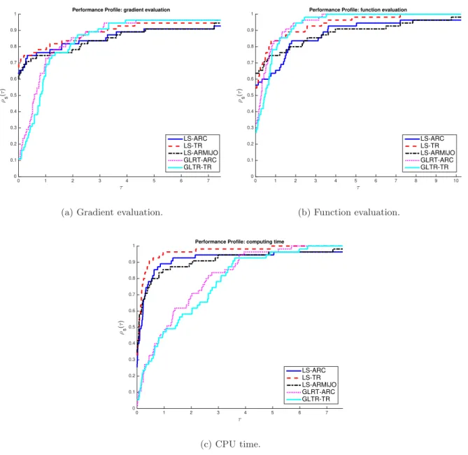
We present the obtained performance profiles in Figure 1. Regarding the gradient evaluation (i.e., outer iteration) performance profile, see Figure 1(a), LS approaches are the most efficient among all the tested solvers (in more 60% of the tested problems LS methods perform the best, while GLRT-ARC and GLTR-TR are performing better only in less than 15%). When it comes to robustness, all the tested approaches exhibit good performance, GLRT-ARCand GLTR-TR are slightly better.
For function evaluation performance profile given by Figure 1(b), GLRT-ARC and GLTR-TR show a better efficiency but not as good as LS methods. In fact, in more than 50% of the tested problems LS methods perform the best while GLRT-ARC and GLTR-TR are better only in less than 35%. The robustness of the tested algorithms is the same as in the gradient evaluation performance profile.
In terms of the demanded computing time, see Figure 1(c), as one can expect,GLRT-ARCand GLTR-TR are turned to be very consuming compared to the LS approaches. In fact, unlike the LS methods where only an approximate solution of one linear system is needed, the GLRT/GLTR approaches may require (approximately) solving multiple linear systems in sequence.
For the LS approaches, one can see that LS-TR displays better performance compared to LS-ARMIJOon the tested problems. The main difference between the two LS algorithms is the strategy of choosing the search direction whenever gk⊤sQk > 0. In our tested problems, the obtained performance using LS-TR suggests that going exactly in the opposite direction −sQk, whenever sQk is not a descent direction, can be seen as a good strategy compared toLS-ARMIJO.
7
Conclusions
In this paper, we have proposed the use of a specific norm in ARC/TR. With this norm choice, we have shown that the trial step of ARC/TR is getting collinear to the quasi-Newton direction. The obtained ARC/TR algorithm behaves as LS algorithms with a specific backtracking strategy. Under mild assumptions, the proposed scaled norm was shown to be uniformly equivalent to the Euclidean norm. In this case, the obtained LS algorithms enjoy the same convergence and complexity properties as ARC/TR. We have also proposed a second order version of the LS algorithm derived from ARC with an optimal worst-case complexity bound of orderǫ−3/2. Our numerical experiments showed encouraging performance of the proposed LS algorithms.
A number of issues need further investigation, in particular the best choice and the impact of the parameter βk on the performance of the proposed LS approaches. Also, the analysis
τ 0 1 2 3 4 5 6 7 ρs ( τ ) 0 0.1 0.2 0.3 0.4 0.5 0.6 0.7 0.8 0.9
1 Performance Profile: gradient evaluation
LS-ARC LS-TR LS-ARMIJO GLRT-ARC GLTR-TR
(a) Gradient evaluation.
τ 0 1 2 3 4 5 6 7 8 9 10 ρs ( τ ) 0 0.1 0.2 0.3 0.4 0.5 0.6 0.7 0.8 0.9
1 Performance Profile: function evaluation
LS-ARC LS-TR LS-ARMIJO GLRT-ARC GLTR-TR (b) Function evaluation. τ 0 1 2 3 4 5 6 7 ρs ( τ ) 0 0.1 0.2 0.3 0.4 0.5 0.6 0.7 0.8 0.9
1 Performance Profile: computing time
LS-ARC LS-TR LS-ARMIJO GLRT-ARC GLTR-TR (c) CPU time.
Figure 1: Performance profiles for 62 large scale optimization problems (i.e., 1000≤n≤10000). defining a line-search method with an optimal worst-case complexity bound of order ǫ−3/2. It would be interesting to confirm the potential of the proposed line search strategy compared to the classical LS approaches using extensive numerical tests.
References
[1] E. Bergou, Y. Diouane, and S. Gratton. On the use of the energy norm in trust-region and adaptive cubic regularization subproblems. Comput. Optim. Appl., 68(3):533–554, 2017.
[2] E. G. Birgin, J. L. Gardenghi, J. M. Mart´ınez, S. A. Santos, and Ph. L. Toint. Worst-case evaluation complexity for unconstrained nonlinear optimization using high-order regularized models. Math.
Program., 163(1):359–368, 2017.
[3] E. G. Birgin and J. M. Mart´ınez. The use of quadratic regularization with a cubic descent condition for unconstrained optimization. SIAM J. Optim., 27(2):1049–1074, 2017.
[4] C. Cartis, N. I. M. Gould, and Ph. L. Toint. Adaptive cubic overestimation methods for uncon-strained optimization. Part II: worst-case function- and derivative-evaluation complexity. Math. Program., 130(2):295–319, 2011.
[5] C. Cartis, N. I. M. Gould, and Ph. L. Toint. Adaptive cubic regularisation methods for unconstrained optimization. Part I: Motivation, convergence and numerical results. Math. Program., 127(2):245– 295, 2011.
[6] C. Cartis, N. I. M. Gould, and Ph. L. Toint. Optimality of orders one to three and beyond: char-acterization and evaluation complexity in constrained nonconvex optimization. Technical report, 2017.
[7] C. Cartis, Ph. R. Sampaio, and Ph. L. Toint. Worst-case evaluation complexity of non-monotone gradient-related algorithms for unconstrained optimization. Optimization, 64(5):1349–1361, 2015. [8] A. R. Conn, N. I. M. Gould, and Ph. L. Toint. Trust-Region Methods. SIAM, Philadelphia, PA,
USA, 2000.
[9] F. E. Curtis, D. P. Robinson, and M. Samadi. A trust region algorithm with a worst-case iteration complexity ofO(ǫ−3/2) for nonconvex optimization. Math. Program., 162(1):1–32, 2017.
[10] J. E. Dennis and R. B. Schnabel. Numerical methods for unconstrained optimization and nonlinear equations. Prentice-Hall Inc, Englewood Cliffs, NJ, 1983.
[11] E. D. Dolan and J. J. Mor´e. Benchmarking optimization software with performance profiles. Math. Program., 91(2):201–213, 2002.
[12] N. I. M. Gould, D. Orban, and Ph. L. Toint. GALAHAD, a library of thread-safe fortran 90 packages for large-scale nonlinear optimization. ACM Trans. Math. Softw., 29(4):353–372, 2003.
[13] N. I. M. Gould, D. Orban, and Ph. L. Toint. CUTEst: a constrained and unconstrained testing environment with safe threads for mathematical optimization.Comput. Optim. Appl., 60(3):545–557, 2015.
[14] S. Gratton, A. Sartenaer, and Ph. L. Toint. Recursive trust-region methods for multiscale nonlinear optimization. SIAM J. Optim., 19(1):414–444, 2008.
[15] A. Griewank. The modification of Newton’s method for unconstrained optimization by bounding cubic terms. Technical Report NA/12, Department of Applied Mathematics and Theoretical Physics, University of Cambridge, United Kingdom, 1981.
[16] J. M. Mart´ınez and M. Raydan. Cubic-regularization counterpart of a variable-norm trust-region method for unconstrained minimization. J. Global Optim., 68(2):367–385, 2017.
[17] Y. Nesterov. Introductory Lectures on Convex Optimization. Kluwer Academic Publishers, 2004. [18] Y. Nesterov and B. T. Polyak. Cubic regularization of Newton’s method and its global performance.
Math. Program., 108(1):177–205, 2006.
[19] C. C. Paige and M. A. Saunders. Solution of sparse indefinite systems of linear equations. SIAM J. Numer. Anal., 12(4):617–629, 1975.