A data-driven optimization-based approach for siting and sizing of electric taxi charging stations

(1)

Civil, Construction and Environmental Engineering

Publications

Civil, Construction and Environmental Engineering

4-2017

A data-driven optimization-based approach for

siting and sizing of electric taxi charging stations

Jie Yang

Southeast University, China

Jing Dong

Iowa State University, [email protected]

Liang Hu

Iowa State University, [email protected]

Follow this and additional works at:

https://lib.dr.iastate.edu/ccee_pubs

Part of the

Civil Engineering Commons, and the

Transportation Engineering Commons

The complete bibliographic information for this item can be found at

https://lib.dr.iastate.edu/

ccee_pubs/203. For information on how to cite this item, please visit

http://lib.dr.iastate.edu/

howtocite.html.

This Article is brought to you for free and open access by the Civil, Construction and Environmental Engineering at Iowa State University Digital Repository. It has been accepted for inclusion in Civil, Construction and Environmental Engineering Publications by an authorized administrator of Iowa State University Digital Repository. For more information, please [email protected].

(2)

A data-driven optimization-based approach for siting and sizing of electric

taxi charging stations

Abstract

This paper presents a data-driven optimization-based approach to allocate chargers for battery electric vehicle (BEV) taxis throughout a city with the objective of minimizing the infrastructure investment. To account for charging congestion, anM/M/x/squeueing model is adopted to estimate the probability of BEV taxis being charged at their dwell places. By means of regression and logarithmic transformation, the charger allocation problem is formulated as an integer linear program (ILP), which can be solved efficiently using Gurobi solver. The proposed method is applied using large-scale GPS trajectory data collected from the taxi fleet of

Changsha, China. The key findings from the results include the following: (1) the dwell pattern of the taxi fleet determines the siting of charging stations; (2) by providing waiting spots, in addition to charging spots, the utilization of chargers increases and the number of required chargers at each site decreases; and (3) the tradeoff between installing more chargers versus providing more waiting spaces can be quantified by the cost ratio of chargers and parking spots.

Keywords

Electric taxis, Charging infrastructure planning, GPS trajectory data, Integer programing, Queueing model Disciplines

Civil Engineering | Transportation Engineering Comments

This is a manuscript of an article published as Yang, Jie, Jing Dong, and Liang Hu. "A data-driven optimization-based approach for siting and sizing of electric taxi charging stations."Transportation Research Part C:

Emerging Technologies77 (2017): 462-477. DOI:10.1016/j.trc.2017.02.014. Posted with permission. Creative Commons License

This work is licensed under aCreative Commons Attribution-Noncommercial-No Derivative Works 4.0 License.

(3)

1

A Data-Driven Optimization-Based Approach for Siting and Sizing of

1

Electric Taxi Charging Stations

2

Jie Yang

a,∗

,

Jing Dong

b

, Liang Hu

b

3

a _{Development Research Institute of Transportation Governed by Law, Southeast University, Nanjing 210096,} 4

China 5

b _{Department of Civil, Construction and Environmental Engineering, Iowa State University, Ames, IA 50011,} 6

United States 7

8

Citation: Yang, J., Dong, J., & Hu, L. (2017). A data-driven optimization-based approach for siting and sizing of

9

electric taxi charging stations. Transportation Research Part C: Emerging Technologies, 77, 462-477.

10

∗_{Corresponding author}

Postal address: Law school, No. 2 Sipailou, Nanjing, Jiangsu, China, 210096 E-mail address: [email protected]

(4)

2

Abstract 1

This paper presents a data-driven optimization-based approach to allocate chargers for battery electric 2

vehicle (BEV) taxis throughout a city with the objective of minimizing the infrastructure investment. 3

To account for charging congestion, an

M M x s

/ / /

queueing model is adopted to estimate the 4

probability of BEV taxis being charged at their dwell places. By means of regression and logarithmic 5

transformation, the charger allocation problem is formulated as an integer linear program (ILP), which 6

can be solved efficiently using Gurobi solver. The proposed method is applied using large-scale GPS 7

trajectory data collected from the taxi fleet of Changsha, China. The key findings from the results 8

include the following: (1) the dwell pattern of the taxi fleet determines the siting of charging stations; 9

(2) by providing waiting spots, in addition to charging spots, the utilization of chargers increases and 10

the number of required chargers at each site decreases; and (3) the tradeoff between installing more 11

chargers versus providing more waiting spaces can be quantified by the cost ratio of chargers and 12

parking spots. 13

(5)

3

Keywords 1

Electric taxis; Charging infrastructure planning; GPS trajectory data; Integer Programing; Queueing 2

model 3

(6)

4

1. Introduction 1

Replacing conventional gasoline vehicles (CGVs) with alternative fuel vehicles, such as battery electric 2

vehicles (BEVs), offers an appealing chance to reduce greenhouse gas (GHG) emissions and other 3

harmful pollutants in highly populated urban areas (Buekers et al., 2014; Yuksel and Michalek, 2015) . 4

However, the fear that the vehicle has insufficient range to reach the destination, referred to as range 5

anxiety, has been shown to be a significant obstacle to market acceptance of BEVs (Neubauer and 6

Wood, 2014; Rauh et al., 2014). One way to mitigate range anxiety is through the deployment of public 7

charging infrastructure, but high costs of equipment and installation limit the coverage of the charger 8

network (Agenbroad and Holland, 2014; Peterson and Michalek, 2013; Schroeder and Traber, 2012). 9

Thus, it is vital to place and size new charging stations based on charging demands, so as to best utilize 10

limited resources. 11

Various facility location models have been proposed to optimize the layout of hydrogen or gas 12

refueling stations (Aikens, 1985; Church and Velle, 1974; Kuby et al., 2009; Nicholas, Handy, and 13

Sperling, 2004; Wang and Lin, 2009). But most of the existing facility location models cannot be 14

applied to optimizing the location of charging stations for the following two reasons: (1) The placement 15

and sizing of hydrogen and gas stations are usually under certain restrictive conditions for 16

environmental, health, and safety reasons (Kuby et al., 2009), while the conditions for siting chargers 17

are more flexible. It is common to install chargers in parking garages, curbside, and in surface parking 18

lots, so that BEVs can be charged at their dwell places, such as home, work places, and commercial 19

places (Pearre et al., 2011; Tian et al., 2014; Zou et al., 2016). (2) Unlike CGVs, it generally takes a 20

long time to charge BEVs, ranging from 30 minutes to several hours, resulting in a long waiting time 21

for incoming BEVs if all the chargers are occupied (Foley et al., 2010; Li et al., 2015). Waiting for 22

charging is usually an unpleasant experience for BEV drivers. Drivers might have taken a detour and 23

traveled some extra distance to reach the charging station due to limited accessibility, creating an even 24

worse user experience. Detours and waiting times for charging hinder the adoption of BEVs. If BEVs 25

can be charged during their dwell time without behavioral changes—that is, if the time between two 26

consecutive trips can be utilized for charging—consumers are more likely to adopt the BEV technology. 27

In this paper, we investigate the following problem: given daily travel and dwell patterns (including 28

dwell locations, dwell time, and arrival rates) of a fleet of taxis, determine where to deploy new charging 29

stations and how many chargers to install at each station. The objective is to minimize the overall 30

infrastructure investment while satisfying the charging demand. Dwell patterns of potential BEVs are 31

derived from trajectories of over 7,910 taxis whose travel activities were recorded for one week. In 32

particular, to account for charging congestion, an

M M x s

/ / /

queueing model is adopted to estimate 33

the waiting time and the fraction of customers who are turned away. The probability that electric taxis 34

can be charged at their dwell places during the day is considered as the model constraint, and the 35

objective is to minimize the total cost of building charging stations and installing chargers. In general, 36

optimizing the performance of queue systems is a difficult problem because of the nonlinear relationship 37

of the performance metrics as functions of the arrival and service rates, and the computational time 38

increases exponentially with the size of the problem (Bertsimas et al., 1994; Mung et al., 2002). In the 39

proposed charger location problem, hundreds of charging stations need to be sited in the city, and 40

multiple chargers need to be assigned to each station. Thus, solving the nonlinear mixed integer program 41

is computationally demanding. An approximation method is presented to transform the formulation to 42

an integer linear program (ILP), which can be solved efficiently. In summary, the main contributions 43

of this paper include the following: (1) develop queueing models to describe charging congestion based 44

on taxis’ dwell patterns observed from GPS tracked trajectory data; (2) formulate the charger allocation 45

problem as an integer linear program, considering charging congestion phenomenon; and (3) investigate 46

the tradeoff between installing more chargers versus providing more waiting spaces and the impact of 47

charger power on waiting time. 48

(7)

5

The rest of the paper is organized as follows. Section 2 presents an overview of related work, 1

followed by problem statement and assumptions in Section 3. The optimization model and the integer 2

program formulation are presented in Section 4. Results and conclusions are summarized in Section 5 3

and 6, respectively. 4

2. Literature review 5

To help policy makers and investors efficiently allocate charging resources, various mathematical 6

models have been developed for charging infrastructure planning. For example, Frade et al. (2011) used 7

a maximal covering model to optimize the location of charging stations in Lisbon, Portugal, with the 8

objective of maximizing demand coverage. Feng et al. (2012) proposed a method for charging station 9

planning using weighted Voronoi diagram. Based on the quantified cost for detour charging, the road 10

network of planning area is partitioned by Voronoi diagram so as to minimize the users’ travel cost. He 11

et al. (2016) compared three classic facility location models and found the p-median model was more 12

effective than the set covering model and the maximal covering location model for locating electric 13

vehicles (EV) charging facilities. Li et al. (2016) developed a multi-period multipath charging station 14

location model that captured the dynamics in the topological structure of network, formulated the model 15

as a mixed integer program, and solved it by genetic algorithm. He et al. (2015) formulated the problem 16

of optimally locating public charging stations within a budget limit as a bi-level mathematical program 17

and solved the problem using a genetic algorithm. Guo et al. (2016) established a network-based multi-18

agent optimization model for planning fast charging stations that simultaneously captured the selfish 19

behaviors of individual investors and travelers and their interactions. The model was solved based on 20

variational convergence theorems. Ghamami et al. (2016) developed a mixed integer program with 21

nonlinear constraint to configure charging infrastructure along highway corridors. The model minimizes 22

the total system cost and considers the realistic patterns of O–D demands and flow-dependent charging 23

delay. Based on a tour-based equilibrium framework, Wang et al. (2016) considered a special EV 24

network composed of fixed routes for an electric bus fleet and optimized the deployment of recharging 25

stations and recharging schedule so as to ensure an electric bus can be charged when it stops within a 26

pre-specified duration. 27

Travel survey data offer an insight into the charging demand and are usually taken as an indicator 28

of the deployment of charging infrastructure. With regard to the studies based on travel survey, Chen 29

et al. (2013) formulated a mixed integer programming problem to optimally allocate a constrained 30

number of charging stations based on the parking information from over 30,000 personal-trip records 31

collected by household travel survey in Seattle, Washington, United States. Assisted by three spatial 32

data sets, including the National Household Travel Survey (NHTS) data, Aultman-Hall et al. (2012) 33

identified optimal charging locations in the rural areas in Vermont, United States. In comparison with 34

traditional travel survey data, Global Positioning Systems (GPS) tracked travel survey data contain 35

more accurate information about trip length, dwell place, and dwell duration of each vehicle, thus 36

providing a way to estimate the spatial and temporal distribution of charging demand. Individual GPS 37

tracked trajectory data, collected from conventional gasoline vehicles and representing real world travel 38

activities, have been used to site public charging stations in previous studies. In Dong et al. (2014)a 39

charger location optimization problem considering daily travel activity constraints was proposed based 40

on GPS-based travel survey data collected in the greater Seattle metropolitan area. 41

Since it is common for taxis to install GPS devices for the purpose of navigation and operational 42

monitoring, taxi trajectories become a major data source to examine the market potential of BEV taxis 43

(Baert and Kort, 2013; Chrysostomou et al., 2016; Tian et al., 2014; Wang et al., 2015; Yang et al., 44

2016) and optimize the siting of public charging stations (Tu et al., 2016, Shen et al., 2016). Taxi fleet 45

has some desirable features for deploying plug-in electric vehicles. Fuel cost savings are significant, as 46

taxis are driven heavily; thus, the payback period tends to be shorter. Cai et al. (2014) demonstrated the 47

potential public charging stations by extracting public parking ‘‘hotspots” from taxi trajectory data in 48

(8)

6

Beijing, China. This research was expanded by Shahraki et al. (2015), in which an optimization model 1

was developed to determine optimal charger allocation, with the objective of maximizing electrified 2

fleet vehicle miles traveled (VMT) of plug-in hybrid electric vehicles (PHEVs). Based on an event-3

based simulation, Sellmair and Hamacher (2014) proposed an algorithm to optimize the number of 4

charging stations per taxi stand based on real world driving patterns of conventional taxis in Munich, 5

Germany. The objective was to maximize economic benefit of the entire system including BEV taxi 6

drivers and charging station investors. In Jung et al. (2014) a bi-level simulation-optimization model 7

was proposed to allocate chargers for a fleet of 600 shared-taxis in Seoul, Korea, with an objective of 8

minimizing the queue delay. Ahn and Yeo (2015) proposed an Estimating the Required Density of EV 9

Charging (ERDEC) stations model to estimate the optimal density of charging stations aiming at 10

minimizing the range anxiety based on taxi trajectories in Daejeon City, Korea, which was a pioneering 11

work considering charging queueing. Using the real-world BEV taxi trajectory data collected from 12

Shenzhen, China, Li et al. (2015) built an optimization framework to find the optimal locations to site 13

stations and the optimal assignment of chargers, which also took charging congestion into consideration. 14

The objective was to minimize the average time to find the charging stations and the waiting time for 15

an available charger. 16

In summary, the optimal layout of charging stations is mainly generated using two types of 17

approaches: (1) Without pre-defined candidate sites, the charging station location optimization is 18

considered as a set covering problem based on the configuration of the road network in the study area 19

(e.g., Frade et al., 2011, Feng et al., 2012, Ahn and Yeo, 2015). The drawback of this approach is that 20

it may be impracticable to install chargers at certain locations. (2) Given a set of candidate sites, 21

including existing charging, gas, or hydrogen refueling stations, new stations or chargers are assigned 22

to the study area with a limited budget (e.g. Cai et al., 2014, Jung et al., 2014, Li et al., 2015). As 23

mentioned above, the distribution characteristics of gas and hydrogen stations are different from those 24

of charging stations. Moreover, in the early stage of the BEV market, charging stations are scarce across 25

the city. With more BEVs on the road, more chargers will be scattered all over the city, and the model 26

complexity is increased. The reason our research focused on dwell charging is that, first, the dwell 27

places are supposed to have desired space for parking, which can be equipped with chargers; second, 28

the average dwell time can be considered as the indicator of charger power, i.e., fast chargers are 29

preferred by the stations with shorter dwell time and vice versa. 30

Charging congestion is another concern of this paper. The waiting time may be significant if all 31

the chargers are occupied during the peak hours, especially at the popular dwell sites. Hosseini and 32

MirHassani (2015) developed a recharging station location model with queue considering capacity, 33

recharging time, and waiting time, and solved the problem using a heuristic algorithm. In the context 34

of predicting EVs’ charging demand and its impacts on power grid, the charging congestion effect is 35

modeled using queueing theory. In Ghamami et al. (2016) the average waiting time for charging was 36

computed using deterministic queueing theory. The most widely-adopted queueing model is

M M s

/ /

, 37

assuming that both BEV arrival rate λ and charging service rate µ follow Poisson distributions and 38

that a vehicle will join the queue no matter how long the queue is (Akbari and Fernando, 2015; Bae and 39

Kwasinski, 2012; Qiu et al., 2013; Said et al., 2013; Said, 2015). To account for limited waiting spaces, 40

Fan et al. (2015) applied an

M G x s

/ / /

queueing model, which assumes a general service time 41

distribution and at most

s

BEVs can be accommodated at a station. In this paper, an

M M x s

/ / /

42

queueing model is adopted, which assumes Poisson-distributed arrival and service rates with

x

43

chargers and

s

-

x

waiting spaces. 44

Due to the computational complexity of larger-scale network optimization, little research has been 45

done to study the problem of siting and sizing charging stations simultaneously considering charging 46

congestion. This paper presents a data-driven optimization-based approach for charging infrastructure 47

planning using extensive vehicle activity data. 48

(9)

7

3. Problem statement and assumptions 1

3.1. Problem statement

2

Given a set of candidate sites for installing public charging stations

J

=

{1,2, , }



N

that are favorable 3

dwell places of taxi drivers, a set of BEVs

I

=

{1,2, , }



M

that need to be charged at public charging 4

stations at least once a day, and the probabilities that BEVs can be charged during dwell time without 5

travel pattern changes, the problem is to find optimal locations of charging stations and optimal 6

assignment of chargers to each station, so as to minimize the total investment of public charging 7

infrastructure. 8

The charging demand is estimated based on vehicles’ dwell patterns extracted from GPS 9

trajectories of taxis in Changsha, China, collected from 0:00 on October 8, 2015, to 23:59 on October 10

14, 2015 (local time). By the end of 2014, there were 7,957 taxis operating in Changsha. It is required 11

by the local government that GPS devices are installed on all taxis for monitoring purpose. Thus, the 12

dataset includes the entire taxi fleet in Changsha, with some missing data due to data collection and 13

transmission errors. A GPS signal is captured roughly every 10 seconds for each taxi. The data include 14

time-stamped location (i.e., longitude and latitude), spot speed, azimuth, and operational status (i.e., 15

empty or occupied). All trajectories were cleaned by removing invalid points caused by data recording 16

or transmission errors. 17

The study area is partitioned into a number of equal size cells first. Each cell has a quadrate edge 18

of 0.005° latitude and longitude, approximately equivalent to 0.5×0.5 km2_{. If the GPS records indicate} 19

a vehicle dwelling in the same cell for more than 20 minutes, a dwell event of BEV

i

in cell

j

is 20

labeled. The study area (i.e., 27°~29° N, 111°~115° E) is divided into 320,000 non-overlapping square 21

cells. For each cell, the number of dwell events is counted. There are 2,460 valid cells that have records 22

of taxis parked during the one-week period. It is possible that some of the dwell locations are drivers’ 23

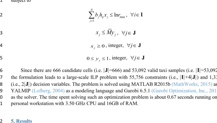
home locations, for which the number of daily dwell events is relatively low. Fig. 1 presents the 24

frequency distribution of the number of daily dwell events per cell. 72.7% of the valid cells have less 25

than 5 daily dwell events. It is comparatively uneconomical to install public charging stations in places 26

that are not attractive to taxi drivers. Thus, only the popular cells, where on average at least 5 dwell 27

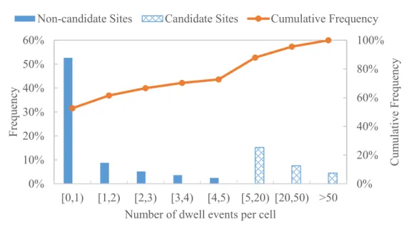
events occurred per day, are considered as candidates for installing public charging stations. Fig. 2 28

shows the spatial distribution of valid cells. There are 666 cells with a daily arrival rate no less than 5 29

veh/day on average, and these are selected as the candidate sites. The selected cells are mostly located 30

in the densely populated area of the inner city. The most popular dwell site is located near Huanghua 31

Airport and far from downtown. It has 10,777 dwell events weekly, with an average frequency of nearly 32

64 per hour. A charging queue and congestion problem might be observed if the taxi fleet is replaced 33

by BEVs. 34

Place Fig. 1 about here 35

A taxi with complete whole-day consecutive trip records is considered a valid sample. Identified 37

from GPS trajectories, there are 53,092 valid taxis with 185,404 dwell events occurring at the selected 38

666 cells over the one-week period. During the dwell time, taxi drivers usually have a meal, change 39

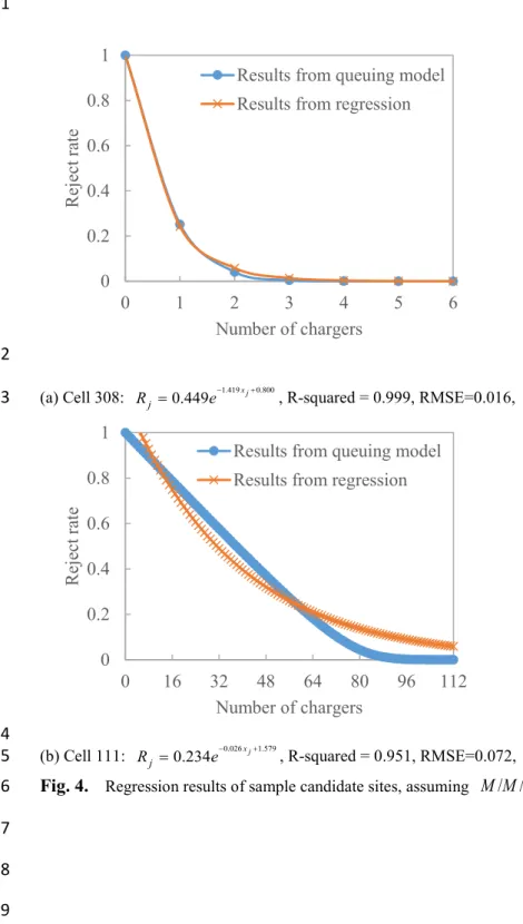
shift, or refuel the vehicle. Fig. 3 shows the number of dwell sites at which one driver would dwell in a 40

day. 15.86% of the taxis dwell at the same sites during the day. For taxis that dwell at multiple sites, if 41

they are turned away at one site, it is possible for them to be charged at the next dwell location. Thus, 42

the allocation of chargers can be optimized based on taxis’ dwell patterns. 43

3.2. Assumptions

(10)

8

3.2.1. Queueing theory for charging system

1

When a driver arrives at a charging station and finds all chargers are occupied, he/she can either wait 2

or decide not to charge at this location. Assume that, at each charging station, the arrival rate,λ, follows 3

a Poisson distribution and the service time,1/

µ

, follows an exponential distribution. The waiting line 4

priority rule of the system is first-come, first-served. Hence, the charging congestion problem can be 5

formulated as the Markovian queueing system with a finite number of chargers,

x

, and a finite capacity, 6

s

, symbolically denoted by

M M x s

/ / /

. 7

If

s

is equal to the number of chargers x, that is, an arriving BEV leaves the system without 8

waiting for service if all chargers are busy, we denote it as

M M x x

/ / /

(i.e., no waiting spaces). If

s

9

is greater than

x

, the arriving BEV will be rejected if the maximum system capacity is reached; 10

otherwise, it will wait in line for service. We denote this queueing system as

M M x K

/ / /

, where

K

11

is the maximum number of customers that can be accommodated in the system (i.e., number of chargers 12

plus number of waiting spaces). The maximum queue size,

K x

−

, can be considered as the number of 13

parking spaces provided for customers waiting for a charger. It is assumed that, for the

M M x K

/ / /

14

queueing system, every five chargers are equipped with one parking spot for waiting. Thus, the system 15

capacity can be computed by Eq. (1), where the parameter

δ

is set as 5. 16 / K x= + _x

δ

_ (1) 17 3.2.2. Service time 18

Service time, or charging time, varies based on the type of chargers. In addition, BEV drivers might not 19

move their vehicles until they finish their dwell activities even if the battery is fully charged. Therefore, 20

the average service times at cell

j

, denoted as

t

_j (unit: day), are estimated in two ways: (1) Drivers 21

are assumed to move their vehicles when they depart; that is, the service time is estimated based on the 22

dwell time obtained from the trajectory data. The service rate, denoted as

µ

₀_j (unit: veh/day), is 23

computed as

µ

₀_j =

1/

t

_j. (2) The service time is determined by the charging power. It is noted that 24

not all the charging power can be directly transferred to battery energy, and a portion of the power is 25

lost during the charging process. Let α denote the charging efficiency. In this paper, we setα as 1.3 (Nie 26

and Ghamami, 2013). For example, if the input charging power is 104 kW, the effective charging power 27

is 80 kW. Assuming the battery capacity is 40 kWh, it takes 30 minutes to fully charge the battery if 28

using an effective charging power of 80 kW, and it takes 180 minutes with an effective charging power 29

of 13.3 kW. Six effective charging powers are taken into account: 80, 40, 26.7, 20, 16, and 13.3 kW. 30

Accordingly, the average service time of each station is assumed as 30, 60, 90, 120, 150, and 180 31

minutes, and the service rate

µ

is 48, 24, 16, 12, 9.6, and 8 vehicles per day, respectively. Since we 32

do not estimate initial state of charge (SOC) of BEVs when they arrive at the stations, regardless of 33

what the SOC is after charging, in case (1) BEVs are assumed to be unplugged and removed from the 34

charger when their dwell time runs out, and in case (2) BEVs will be unplugged as soon as the assumed 35

service time runs out. 36

3.2.3. Charging demand

37

The sites where taxis frequently dwell are likely to have ample parking spaces to install chargers and 38

thus are selected as candidate sites. The number of average daily dwell events occurring at these 39

locations can be derived from the GPS trajectory data. In this paper, the average daily charging demand 40

(i.e., daily arrival rate) of cell

j

, denoted as

λ

_j (unit: veh/day), is assumed to be the average number 41

of daily dwell events occurring in the cell. At an early market with a small number of BEV taxis on the 42

road, the charging demand is likely less than the number of dwell events. As the number of BEVs on 43

the road increases, the demand for dwell charging increases too. In particular, Beijing has recently 44

(11)

9

announced that all internal combustion engine (ICE) taxis will be replaced by BEVs by 2020 (DRC of 1

Beijing, 2016), in which case all the dwell taxis might use the chargers. Furthermore, if the chargers are 2

open to private BEVs and other commercial BEVs, the charging demand could exceed the number of 3

daily taxi dwell events. Predicting the future charging demand for each cell is beyond the scope of this 4

research. Since taxi dwell patterns represent the spatial distribution attributes of charging demand, for 5

simplicity we assume the charging demand

λ

_j follows the taxis arrival patterns at the charging 6 stations. 7 4. Methodology 8 4.1. Formulation 9

4.1.1. Charging reject rate

10

As mentioned above, valid BEV samples are supposed to dwell at least at one candidate site during the 11

day. The factors indicating that BEVs are being charged successfully during their dwell events include 12

(1) chargers are installed at the dwell places, and (2) chargers or waiting spaces are available when 13

BEVs arrive. 14

Cell

j

is assumed as the dwell place for BEV

i

. Once BEV

i

arrives at cell

j

, the probability 15

that neither chargers nor waiting spaces are available is denoted as R_j (R_j∈[0, 1]). The probability 16

of BEV

i

being turned away at cell

j

is considered as r_ij (r_ij∈[0, 1]), where rij =Rj. Obviously, 17

if BEV

i

does not have the opportunity to park at cell

j

during the day, the reject rate r_ij equals 1.

18

The relationship between r_ij and R_j can be written by Eq. (2) 19 ij h ij j

r

=

R

(2) 20

where h_ijis a binary variable indicating whether BEV

i

dwells at cell

j

. If it does, hij =1;

21

otherwise, hij =0.

22

Define

W

_i as the daily reject rate of BEV

i

, which is the multiplication of reject probabilities 23

that BEV

i

is turned away at cell

j

(

∀ ∈

j

J

) (Eq. (3)). The probability of BEV

i

being charged 24

at least once in a day during its dwell events is then

1

−

W

_i. 25 1 N i ij j

W

r

=

∏

(3) 26

The tradeoff between BEVs daily reject rate and charger network coverage is as follows. If

W

_i

=

1

, 27

it is impossible for BEV

i

to take the dwell time for charging during the day because there is no 28

charging station wherever it dwells. Therefore, it has no choice but to detour for charging, which 29

increases BEV drivers’ cost. As to BEV taxis, detour charging not only leads to extra travel distance 30

but also reduces the daily operating time and decreases taxi drivers’ revenue. If

W

_i

=

0

, wherever BEV 31

i

dwells, it can always be charged because of adequate charger network coverage, which, of course, 32

requires enormous infrastructure investment. The daily reject rate

W

_i can be considered as a measure 33

of service quality of charger coverage and can be calculated based on queueing theory. 34

(12)

10

Denote p_s as the probability of a full system in which prospective BEV drivers are turned away. 1

It is widely known as Erlang’s loss formula and determined by the utilization ratio ρj =λ µj / j and

2

the number of chargers

x

_j. The probability p_s for an

M M x s

/ / /

system is given by Gross (2008) 3 0 ! ρ − = s s s x p p x x (4) 4

where p₀ represents the probability that no customers are in the system, and it equals 5 1 1 1 0 0 ₁ 1 0 (1 ) _, ₁ ! !(1 ) ( 1) , 1 ! !

ρ

− − + − = − − =  −  _ + _ ≠ −   =     + − + =      

∑

x s x n x s s n s n x x s n n x p s x n x (5) 6

where

ρ

is the ratio of arrival rate

λ

and service rate

µ

, and ρ_s is the average utilization of the 7 system 8 s _x _x ρ λ ρ µ = = (6) 9

Thus, the reject rate at cell

j

(namely,R_j) can be expressed as

10 ( , ) 0 1 0

ρ

>  =  ₌  s j j j j j p x x R _x (7) 11

The daily reject rate

W

_i can be calculated using Eq. (2)–(7). Define

r

_max as the maximum 12

allowable daily reject rate for each BEV (i.e., the probability that BEVs cannot be charged at any of the 13

dwell places during the day). The service quality constraint

W r

_i

≤

_max(

∀ ∈

i

I

) should be satisfied when 14

optimize the siting and sizing of charging stations. 15

4.1.2. Optimization model

16

Let binary variable

y

j denote the deployment configuration for cell

j

. When

y

j

=

1

, at least one

17

charger is installed at cell

j

; otherwise, no charging station is installed at cell

j

. Let integer variable 18

j

x

denote the number of chargers installed at cell

j

. The infrastructure cost includes a fixed cost of 19

deploying a new charging station (denoted as

V

, unit: yuan per station) and the unit cost of a charger 20

(denoted as

C

, unit: yuan per charger). The charger cost

C

varies greatly depending on the type of 21

chargers. Single-port chargers with AC Level 2 capabilities cost ￥6500–13,000 excluding installation 22

and potential electrical upgrades in order to provide the appropriate outlet near the EV parking spot, 23

while the cost of DC fast chargers can be as high as ￥65,000–260,000 depending on the features and 24

brands (Delucchi et al., 2013; Schroeder and Traber, 2012). The fixed cost of deploying a new charging 25

station

V

includes the installation cost and permit fee. Unlike home stations, where hardware is the 26

dominant cost, installation is the major contributor to public station cost (60% to 80% of total) 27

(Agenbroad and Holland, 2014). To minimize the investment, the total cost can be expressed as 28

(13)

11 1 1 min ( , ) N _j N _j j j J x y C x V y = = =

∑

+

∑

(8) 1 subject to 2 max

≤

i

W r

,

∀ ∈

i

I

(9) 3

0

j

x

≥

, integer,

∀ ∈

j

J

(10) 4 1 0 0 j 0 j j x y =  _x >₌  (11) 5 4.2. Solution method 6

Optimizing the performance of queueing systems is a difficult task because of the nonlinearity of the 7

performance metrics as functions of the arrival and service rates. In general, the computational time 8

scales exponentially with the problem size. It is computationally demanding to solve the proposed 9

model with 666 queueing systems in the network. Note that the reject probability of an

M M x s

/ / /

10

system is a posynomial function, which has convexity properties (Mung et al., 2002). After a 11

logarithmic transformation, a global optimum solution can be found efficiently. Therefore, the 12

optimization model is reformulated into an integer linear program (ILP). 13

4.2.1. Regression

14

Assuming the reject rate R_j is a function of the number of chargers xj, a series of exponential 15

regression models is set up in the form of

=

b x cj j+ j

j j

R a e

for the purpose of simplifying the computation 16

of reject rate R_j (∀ ∈j J ). The regression coefficients aj, bj , and cj vary with system 17

utilization ρ_j. In the case study, since 666 cells are selected as the candidate sites for deploying 18

charging stations, 666 exponential regression models are developed to quantify the effects of charger 19

counts upon the reject rate. Table 1 lists the statistics of regression coefficients. Regardless of the 20

utilization ρ_j , R-squared values are all above 0.935, which indicates the exponential regression 21

formation is a suitable approximation of the relationship between dependent variables R_j and

22

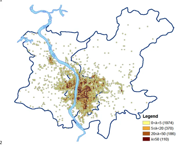
independent variables

x

_j. Fig. 4plots the regression results of two example cells under the assumption 23

of

M M x x

/ / /

queueing system. The system utilization ratios (i.e.,

ρ

j

=

λ µ

j

/

0j) of Cell 308 and Cell

24

111 are 0.34 and 73.82, respectively. Cell 308, located at Guzhang Park along the waterfront, is a newly 25

developed area. This less popular site generates 15 dwell events per day on average. Cell 111, located 26

near Huanghua Airport, is one of the most popular dwell sites and generates 1,540 dwell events daily 27

on average. Obviously, the busier the station is, the more chargers need to be installed so as to satisfy 28

the charging demand. 29

Place Table 1 about here 30

4.2.2. Logarithmic transformation

32

Using the regression models, Eq. (3) can be written as a monomial where variables and coefficients are 33

positive real numbers, and all of the exponents are real numbers: 34

(14)

12 1

(

j j j

)

ij N b x c h i j j

W

a e

+ =

=

∏

(12) 1

The constraint Eq. (9) can be replaced with its logarithm form as 2 max 1 1

ln

ln(

(

) )

= =

≤

−

∑

N

∏

N c hj ij j ij j j j j

b h x

r

a e

(13) 3

Since when xj =0, no chargers are installed at cell

j

, and all the arrival BEVs will be turned 4

away, the reject rate of cell

j

, R_j, should equal 1. However, because the regression model is an

5

approximation of the queueing model, there is no guarantee that when xj =0, Rj= 1. In Eq. (13) we 6

use an approximation that cj

≈

1

j

a e

and, therefore, 1

ln( (

) ) 0

=

∏

N c hj ij j j

a e

.

Hence, constraint Eq. (13) 7 is simplified as Eq. (14) 8 max 1 ln = ≤

∑

N j ij j j b h x r (14) 9

An interesting observation from Table 1is that the average values of coefficients b_j gradually

10

increase with decreasing service rates, while coefficients a_j and cj are roughly unchanged. This 11

supports the approximation in Eq. (14) that only coefficients b_j are included as inequality constraints.

12

As expected, by increasing the number of waiting spaces in

M M x K

/ / /

system, fewer chargers are 13

required in comparison with the

M M x x

/ / /

system. Thus, it is observed that the average values of b_j

14

in

M M x K

/ / /

systems are smaller than those in

M M x x

/ / /

systems. It is speculated that b_j and

15 j

x are positively correlated. For example, based on the assumption of

µ µ

=

0 (i.e., when dwell time

16

is considered as the service time), the average value of b_j is close to that when

µ

=12 veh/day.

17

Specifically, it is because the average dwell time in different candidate sites is about 109.9 minutes and, 18

accordingly, the average system service rate

µ

₀ (i.e.,

µ

₀

=(

∑

_j

µ

0j

)/|

J

|) is equal to 13.1 veh/day.

19

The similar system utilization leads to similar configuration of charger layout, which will be further 20

illustrated in Section 5. 21

Since constraint Eq. (11) is a logic constraint where y_j is binary and xj is a positive integer, a 22

Big-M reformulation is used to convert it into an internal mixed-integer problem. The reformulation is 23

illustrated in Eq. (15), where

M

is chosen as a sufficiently large value. If y_j is 0 (false), xj is 24

guaranteed to be 0; otherwise, x_j is unconstrained.

25

j j

x

≤

My

(15)

26

4.2.3. Integer programming solver

27

The optimization model is formulated in a standard form of ILP as follows: 28 1 1 min ( , ) N j N j j j J x y C x V y = = =

∑

+

∑

29

(15)

13 subject to 1 max 1 ln = ≤

∑

N j ij j j b h x r ,

∀ ∈

i

I

2 j j

x

≤

My

, ∀ ∈j J 3 0 j x ≥ , integer, ∀ ∈j J 4 0≤ yj ≤1, integer, ∀ ∈j J 5

Since there are 666 candidate cells (i.e. |

J

|=666) and 53,092 valid taxi samples (i.e. |

I

|=53,092),

6

the formulation leads to a large-scale ILP problem with 55,756 constraints (i.e.,

|

I

|

+4

|

J

|) and 1,332

7

(i.e., 2|

J

|) decision variables. The problem is solved using MATLAB R2015b

(MathWorks, 2015) and 8

YALMIP (Lofberg, 2004) as a modeling language and Gurobi 6.5.1 (Gurobi Optimization, Inc., 2016) 9

as the solver. The time spent solving such an optimization problem is about 0.67 seconds running on a 10

personal workstation with 3.50 GHz CPU and 16GB of RAM. 11

5. Results 12

5.1. Charging station siting

13

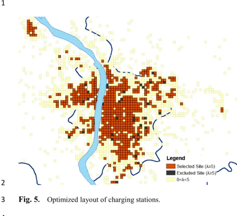
Fig. 5 shows the optimized layout of charging stations in Changsha (the map is zoomed to the inner 14

city). The red cells represent locations where charging stations should be installed, and the black cells 15

represent the candidate sites which are not selected. There are 35 black cells that are excluded from the 16

candidate sites. Various scenarios were tested with the combination of

r

_max ranging from 5% to 25% 17

and ratios of

C

and

V

ranging from 1:0 to 1:10. When

C V

/

equals 1:0, there is no fixed cost 18

associated with a new charging station. Under ideal circumstances, proper electric outlets are already 19

available and investors do not have to pay for installation and the permit fee. However, in most cases, 20

the fixed cost

V

can hardly be avoided and varies greatly depending on the type of charger and location 21

of the charging station. For example, if DC fast chargers are deployed, the fixed cost is likely to be 22

higher because of the transformer upgrades. But no matter how the scenario changes, the configurations 23

of excluded sites remain the same. It might be because the dwell patternH_{=  } h_ij , derived from the 24

GPS dataset, plays a determining role in charging station siting. In the most extreme case, if all the 25

candidate sites have at least one BEV taxi that only dwells once during the day, none of candidate sites 26

will be excluded. 27

Table 2 presents the summary statistics of the selected and excluded cells. Compared with the 29

selected candidates, the excluded cells have lower arrival rates and shorter dwell times, resulting in 30

smaller system utilization. Additionally, the selected cells are not the only charging opportunity for any 31

BEV taxis; the BEVs that dwell there can be charged at other candidate sites. As mentioned in section 32

4.2.2, we assume there is a positive correlation between the coefficients

b

and number of chargers. 33

Obviously, the coefficients

b

of excluded cells are much smaller than those of selected cells. 34

5.2. Charging station sizing

36

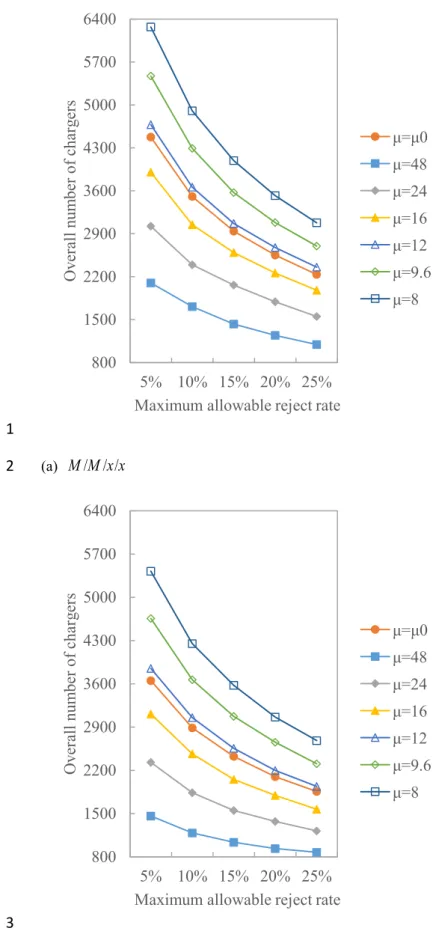
Fig. 6 compares total numbers of chargers needed under different reject rate requirements and charging 37

powers. By increasing the service rate ( i.e., increasing the charging power) or decreasing the reject rate 38

requirement, a lower number of chargers is required to satisfy the charging demand. As mentioned 39

(16)

14

earlier, the assumptions of

µ µ

=

₀ and

µ

=12 veh/day result in similar service rates; thus, the 1

number of required chargers is close in these two scenarios. For a BEV with a range of 200 km and an 2

electricity consumption rate of 0.2 kWh/km (e.g., BYD E6), AC Level 2 chargers with an effective 3

charging power of 20 kW are recommended, assuming the BEVs stay plugged in until their dwell time 4

runs out. Since it takes about 2 hours to fully charge BEV-200km with AC Level 2 chargers, the service 5

rate

µ

is about 12 veh/day. The other observation is that, when using a lower power charger, the 6

curve declines more rapidly with looser reject rate requirements. This is because according to the 7

constraint Eq. (14),the descent rate is determined by the coefficient

b

, which is much smaller at a low 8

service rate than when fast chargers are adopted. 9

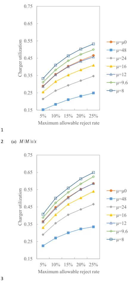
The charger utilization (denoted by

η

) is defined as the ratio of the number of average occupied 11

chargers and all chargers in the system. Fig. 7 presents the results of charger utilization given different 12

scenarios. The value of

η

increases along with the increment of maximum allowable reject rate and 13

the decrement of charging power. For the same maximum allowable reject rate, the queueing system of 14

/ / /

M M x K

requires significantly fewer chargers than the

M M x x

/ / /

system requires. On average, 15

the number of chargers is reduced by 26.7% if fast chargers (i.e.,

µ

=48) are deployed and is reduced 16

by 13.1% if slow chargers (i.e.,

µ

=8) are installed. As waiting space is provided, the value of

η

17

increases by 42.6% and 21.9%, respectively, with

µ

=48 and

µ

=8. 18

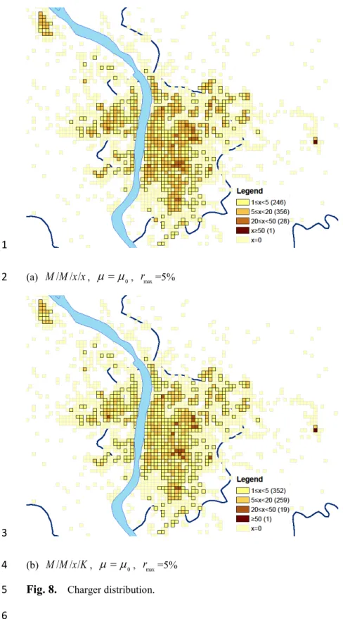
Fig. 8 presents the charger spatial distribution when

µ µ

=

₀ and

r

_max =5%. The mid-sized 20

stations where

5

≤ <

x

20

are most preferred by

M M x x

/ / /

system, while the small-sized stations 21

with fewer than 5 chargers are most favorable for

M M x K

/ / /

system. One super station located near 22

the airport is observed that requires 117 chargers with the

M M x x

/ / /

system and 110 chargers and 22 23

waiting spaces with the

M M x K

/ / /

system. On average 1,540 dwell events occurred every day at that 24

candidate site, and the service rate was 17.07 veh/day. Pragmatically speaking, not all the BEV taxis 25

will charge their batteries during dwell time. However, taking account of the charging demand from 26

private BEVs or other commercial BEVs that travel a long distance to get to the airport, we believe the 27

counted dwell events provide an insight into the real state of charging demand for this area. If the 28

chargers are replaced by more powerful chargers, e.g., with charging power of 80 kW, the service rate 29

rises to 48 veh/day, and the number of chargers can be reduced to 44 units with the

M M x x

/ / /

system 30

or 40 units with the

M M x K

/ / /

system. 31

5.3. Waiting spots and waiting time

33

As can be seen from Fig. 6, the

M M x K

/ / /

system shows its advantage in fewer chargers, although it 34

generates waiting time and needs more parking spaces. Fig. 9 shows the average waiting times when 35

additional parking spots for waiting are available. When

r

_max=5%, since there is a plentiful supply of 36

chargers to satisfy the strict reject rate requirement, the average waiting time is less than 2.5 minutes, 37

which is probably tolerable for most BEV drivers. The most powerful chargers with the service rate of 38

µ

=48 perform best, with the average waiting times ranging from 2.1 minutes (with

r

_max=5%) to 5.9 39

minutes (with

r

_max=25%). As the maximum allowable reject rate goes up, the average waiting time 40

increases, especially for low power chargers. 41

(17)

15

In the

M M x K

/ / /

system we assume every 5five chargers equipped with one parking spot for 1

waiting. Undoubtedly, one charger occupies one parking spot. Let

n

_c denote the number of parking 2

spots used for charging,

n

_w denote the number of parking spots used for waiting, and

n

_sum

= +

n n

_c _w 3

denote the sum of required parking spots. We compare the value of

n

_sum between

M M x x

/ / /

and 4

/ / /

M M x K

systems and present their difference in Fig. 10. From the results we can see that, despite 5

the

M M x K

/ / /

system reducing the number of chargers (i.e., xx xk

c c

n −n ), it requires more parking

6

spots (i.e., xk xx sum sum

n −n ). The waiting space of the system with the most powerful chargers increases

7

drastically, from 44 (with

r

_max=5%) to 423 (with

r

_max=25%), while the fluctuation of slow chargers 8

is not significant. This happens because, with the slow chargers, waiting spots are occupied for longer 9

times compared to fast charging systems and are not influenced by the reject rate. Due to the higher 10

turnover rate of waiting spots in fast charging systems, especially when fewer chargers are required 11

with

r

_max=25%, more waiting space helps to reduce the possibility of BEVs being turned away. 12

The allocation problem for charging facilities is different from that for gas or hydrogen stations. 14

For charging facilities, the question is whether or not the facility should be equipped with more chargers 15

or with enough parking spots for waiting. In general, it depends on the price of one charger (denoted by 16

c

C

) and the price of one parking spot (denoted by

C

_p), and the values of

C

_c and

C

_p vary based 17

on the charger type and the location of stations, respectively. To investigate this question, we define 18

β

as the ratio of

C

_c and

C

_p and

β

₀ as the trade-off parameter where 19 0 1

β

= − = − − − xk xx xk sum sum w xx xk xx xk c c c c n n n n n n n (16) 20 If

β β

>

₀, that is 21

β

=

>

−

xk xx c sum sum xx xk p c c

C

n

C

n

(17) 22

it costs more to install chargers than to provide waiting space given the same required reject rate; 23

otherwise, deploying more chargers is preferred. Table 3 lists the values of

β

₀ under different 24

scenarios. In particular, we assume one parking spot costs ￥40,000 during a charger’s life-cycle, 25

chargers associated with

µ

=48 cost ￥120,000, and chargers associated with

µ

=8 cost ￥4,000. 26

Hence, it is suggested to provide more waiting spots when fast chargers are deployed since

β

=300% 27

and

β

₀ is smaller than 200% when

r

_max

≤

25%. If installing chargers with low charging power and 28

setting

r

_max as 25%,

β

is equal to 100% thereof, and it is more economical to increase the number 29

of chargers. 30

(18)

16 6. Conclusions

1

This paper presents a data-driven optimization model to allocate charging stations and chargers 2

throughout a city with the objective of minimizing overall investment. The proposed approach takes 3

vehicles’ dwell pattern as input and the probability of BEVs being charged during their dwell time as 4

constraints. Charging congestion is taken into consideration and formulated using queueing theory. By 5

means of regression and logarithmic transformation, the optimization model is transformed into an ILP 6

problem and solved by Gurobi solver efficiently. The key findings from the results include the following: 7

(1) The dwell pattern of the taxi fleet determines the siting of charging stations, and 35 out of 666 8

candidate sites do not have to install chargers after optimization. (2) When waiting space is offered, the 9

utilization of chargers can be improved and the number of chargers can be reduced by 13.1% to 26.7%, 10

compared to charging stations with no waiting space. However, it will require more parking spots and 11

increase users’ waiting time. (3) The tradeoff between installing more chargers versus providing more 12

waiting spaces depends on the cost ratio of chargers and parking spots, which varies with the charger 13

power and required reject rate as well. For 20 kW chargers, in order to satisfy at least 95% of the 14

charging demand, it is more economical to install more chargers instead of providing more waiting 15

spaces when the price of chargers is less than 23% of the cost of parking spots. 16

The main caveat of the proposed approach is that it does not account for the SOC when BEVs 17

arrive at charging stations. BEVs with high level of SOC may not charge at their dwell place. Also, 18

depending on the type of chargers and SOC, charging time may vary for different vehicles. Another 19

aspect that needs further research is the penetration rate of BEVs. The dataset tested in this paper 20

captures only the charging demand of potential BEV taxis, while trajectory data collected from other 21

kinds of private or commercial BEVs can be used to better estimate the charging demand and further 22

support the charging infrastructure planning for Changsha. Moreover, due to the lack of land use 23

information, the space limitation of charging and waiting areas at each site is not considered in the 24

model formulation. The proposed model could be further improved if information about the cost of 25

acquiring the land is available. 26

Despite these caveats, the methodology presented in this paper provides a tool for infrastructure 27

providers, city planners, and other stakeholders to determine where charging stations should be located 28

and how many chargers and waiting spaces need to be assigned. 29

Acknowledgments 30

This work was partially supported by the Social Science Foundation of Jiangsu Province of China under 31

project NO. 14FXC001. Y.J. acknowledges the support of the State Scholarship Fund from China 32

Scholarship Council. 33

References 34

Agenbroad, J., Holland, B., 2014. Pulling Back the Veil on EV Charging Station Costs. Rocky 35

Mountain Institute. April 29, 2014. 36

Ahn, Y., Yeo, H., 2015. An Analytical Planning Model to Estimate the Optimal Density of Charging 37

Stations for Electric Vehicles. PloS one 10(11), e0141307. 38

Aikens, C.H., 1985. Facility location models for distribution planning. European Journal of 39

Operational Research 22(3), 263-279. 40

Akbari, H. and Fernando, X., 2015. Modeling and optimization of PHEV charging queues. In 41

Electrical and Computer Engineering (CCECE), 2015 IEEE 28th Canadian Conference on (pp. 42

81-86). IEEE. 43

(19)

17

Aultman-Hall, L., Sears, J., Dowds, J., Hines, P., 2012. Travel Demand and Charging Capacity for 1

Electric Vehicles in Rural States: Vermont Case Study. Transportation Research Record: Journal 2

of the Transportation Research Board(2287), 27-36. 3

Bae, S., Kwasinski, A., 2012. Spatial and temporal model of electric vehicle charging demand. IEEE 4

Transactions on Smart Grid 3(1), 394-403. 5

Baert, R.S.G., Kort, H.J., 2013. Real world experience with operating electric vehicles in the 6

Netherlands, Electric Vehicle Symposium and Exhibition (EVS27), 2013 World, pp. 1-9. 7

Bertsimas, D., Ioannis Ch, P., Tsitsiklis, J.N., 1994. Optimization of Multiclass Queueing Networks: 8

Polyhedral and Nonlinear Characterizations of Achievable Performance. The Annals of Applied 9

Probability 4(1), 43-75. 10

Buekers, J., Van Holderbeke, M., Bierkens, J., Panis, L., 2014. Health and environmental benefits 11

related to electric vehicle introduction in EU countries. Transportation Research Part D: 12

Transport and Environment 33, 26-38. 13

Cai, H., Jia, X., Chiu, A.S.F., Hu, X., Xu, M., 2014. Siting public electric vehicle charging stations in 14

Beijing using big-data informed travel patterns of the taxi fleet. Transportation Research Part D: 15

Transport and Environment 33, 39-46. 16

Chen, T.D., Kockelman, K.M., Khan, M., 2013. The electric vehicle charging station location 17

problem: a parking-based assignment method for Seattle, Transportation Research Board 92nd 18

Annual Meeting pp. 13-1254. 19

Chrysostomou, K., Georgakis, A., Morfoulaki, M., Kotoula, K., Myrovali, G., 2016. Using Big Taxi 20

GPS Data to Investigate Feasibility of Electric Taxis in Thessaloniki, Greece. In Transportation 21

Research Board 95th Annual Meeting (No. 16-3467). 22

Church, R., Velle, C.R., 1974. The Maximal Covering Location Problem. Papers in Regional Science 23

32(1), 101--118. 24

Delucchi, M.A., Yang, C., Burke, A.F., Ogden, J.M., Kurani, K., Kessler, J., Sperling, D., 2013. An 25

assessment of electric vehicles: technology, infrastructure requirements, greenhouse-gas 26

emissions, petroleum use, material use, lifetime cost, consumer acceptance and policy initiatives. 27

Philosophical Transactions of the Royal Society A: Mathematical, Physical and Engineering 28

Sciences 372(2006). 29

DRC of Beijing, Development and Reform Committee of Bejing, 2016. Special planning for charging 30

infrastructure in Beijing (2016-2060). 31

http://www.bjpc.gov.cn/zwxx/tztg/201604/P020160422395177786941.pdf 32

Dong, J., Liu, C., Lin, Z., 2014. Charging infrastructure planning for promoting battery electric 33

vehicles: An activity-based approach using multiday travel data. Transportation Research Part C: 34

Emerging Technologies 38, 44-55. 35

Fan, P., Sainbayar, B., Ren, S., 2015. Operation analysis of fast charging stations with energy demand 36

control of electric vehicles. IEEE Transactions on Smart Grid 6(4), 1819-1826. 37

Feng, L., Ge, S., Liu, H., 2012. Electric Vehicle Charging Station Planning Based on Weighted 38

Voronoi Diagram, 2012 Asia-Pacific Power and Energy Engineering Conference, pp. 1-5. 39

Foley, A.M., Winning, I.J., Gallachoir, B.P.O., 2010. State-of-the-art in electric vehicle charging 40

infrastructure, 2010 IEEE Vehicle Power and Propulsion Conference, pp. 1-6. 41

Frade, I., Ribeiro, A., Gonçalves, G., Antunes, A., 2011. Optimal location of charging stations for 42

electric vehicles in a neighborhood in Lisbon, Portugal. Transportation Research Record: Journal 43

of the Transportation Research Board(2252), 91-98. 44

(20)

18

Ghamami, M., Zockaie, A., Nie, Y., 2016. A general corridor model for designing plug-in electric 1

vehicle charging infrastructure to support intercity travel. Transportation Research Part C: 2

Emerging Technologies 68, 389-402. 3

Gross, D., 2008. Fundamentals of queueing theory. John Wiley & Sons. 4

Guo, Z., Deride, J., Fan, Y., 2016. Infrastructure planning for fast charging stations in a competitive 5

market. Transportation Research Part C: Emerging Technologies 68, 215-227. 6

Gurobi Optimization, Inc., 2016. Gurobi Optimizer Reference Manual. http://www.gurobi.com. 7

He, F., Yin, Y., Zhou, J., 2015. Deploying public charging stations for electric vehicles on urban road 8

networks. Transportation Research Part C: Emerging Technologies 60, 227-240. 9

He, S.Y., Kuo, Y.-H., Wu, D., 2016. Incorporating institutional and spatial factors in the selection of 10

the optimal locations of public electric vehicle charging facilities: A case study of Beijing, 11

China. Transportation Research Part C: Emerging Technologies 67, 131-148. 12

Hosseini, M., MirHassani, S.A., 2015. Selecting optimal location for electric recharging stations with 13

queue. KSCE Journal of Civil Engineering 19(7), 2271-2280. 14

Jung, J., Chow, J.Y.J., Jayakrishnan, R., Park, J.Y., 2014. Stochastic dynamic itinerary interception 15

refueling location problem with queue delay for electric taxi charging stations. Transportation 16

Research Part C: Emerging Technologies 40, 123-142. 17

Kuby, M., Lines, L., Schultz, R., Xie, Z., Kim, J.G., Lim, S., 2009. Optimization of hydrogen stations 18

in Florida using the Flow-Refueling Location Model. International Journal of Hydrogen Energy 19

34(15), 6045-6064. 20

Li, S., Huang, Y., Mason, S.J., 2016. A multi-period optimization model for the deployment of public 21

electric vehicle charging stations on network. Transportation Research Part C: Emerging 22

Technologies 65, 128-143. 23

Li, Y., Luo, J., Chow, C.Y., Chan, K.L., Ding, Y., Zhang, F., 2015. Growing the charging station 24

network for electric vehicles with trajectory data analytics, 2015 IEEE 31st International 25

Conference on Data Engineering, pp. 1376-1387. 26

Lofberg, J., 2004. YALMIP : a toolbox for modeling and optimization in MATLAB, Computer Aided 27

Control Systems Design, 2004 IEEE International Symposium on, pp. 284-289. 28

MathWorks, 2015. MATLAB Version 8.6 (R2015b). Natick, MA, USA. 29

Nicholas, M., Handy S., and Sperling, D., 2004. Using Geographic Information Systems to Evaluate 30

Siting and Networks of Hydrogen Stations. Transportation Research Record: Journal of the 31

Transportation Research Board 1880, 126-134. 32

Mung, C., Sutivong, A., Boyd, S., 2002. Efficient nonlinear optimizations of queuing systems, Global 33

Telecommunications Conference, 2002. GLOBECOM '02. IEEE, pp. 2425-2429 vol.2423. 34

Neubauer, J., Wood, E., 2014. The impact of range anxiety and home, workplace, and public charging 35

infrastructure on simulated battery electric vehicle lifetime utility. Journal of Power Sources 257, 36

12-20. 37

Nie, Y., Ghamami, M., 2013. A corridor-centric approach to planning electric vehicle charging 38

infrastructure. Transportation Research Part B: Methodological 57, 172-190. 39

Pearre, N.S., Kempton, W., Guensler, R.L., Elango, V.V., 2011. Electric vehicles: How much range is 40

required for a day’s driving? Transportation Research Part C: Emerging Technologies 19(6), 41

1171-1184. 42

Peterson, S.B., Michalek, J.J., 2013. Cost-effectiveness of plug-in hybrid electric vehicle battery 43

capacity and charging infrastructure investment for reducing US gasoline consumption. Energy 44

Policy 52, 429-438. 45

Qiu, G.B., Liu, W.X., Zhang, J.H., 2013. Equipment Optimization Method of Electric Vehicle Fast 46

Charging Station Based on Queuing Theory. Applied Mechanics and Materials 291, 872-877. 47

Rauh, N., Franke, T., Krems, J.F., 2014. Understanding the impact of electric vehicle driving 48

experience on range anxiety. Human Factors: The Journal of the Human Factors and Ergonomics 49

Society, 0018720814546372. 50

Said, D., Cherkaoui, S., Khoukhi, L., 2013. Queuing model for EVs charging at public supply 51

stations. In 2013 9th International Wireless Communications and Mobile Computing Conference 52

(IWCMC) (pp. 65-70). IEEE. 53

(21)

19

Said, D, Cherkaoui, S., Khoukhi, L., 2015. Multi-priority queuing for electric vehicles charging at 1

public supply stations with price variation. Wireless Communications and Mobile Computing 2

15(6), 1049-1065. 3

Schroeder, A., Traber, T., 2012. The economics of fast charging infrastructure for electric vehicles. 4

Energy Policy 43, 136-144. 5

Sellmair, R., Hamacher, T., 2014. Optimization of Charging Infrastructure for Electric Taxis. 6

Transportation Research Record: Journal of the Transportation Research Board 2416, 82-91. 7

Shahraki, N., Cai, H., Turkay, M., Xu, M., 2015. Optimal locations of electric public charging stations 8

using real world vehicle travel patterns. Transportation Research Part D: Transport and 9

Environment 41, 165-176. 10

Shen, M., Li, M., He, F., Jia, Y., 2016. Strategic Charging Infrastructure Deployment for Electric 11

Vehicles. UCCONNECT Final Reports. 12

Tian, Z., Yi, W., Chen, T., Fan, Z., Lai, T., Chengzhong, X., 2014. Understanding operational and 13

charging patterns of Electric Vehicle taxis using GPS records, 17th International IEEE 14

Conference on Intelligent Transportation Systems (ITSC), pp. 2472-2479. 15

Tu, W., Li, Q., Fang, Z., Shaw, S.l., Zhou, B., Chang, X., 2016. Optimizing the locations of electric 16

taxi charging stations: A spatial–temporal demand coverage approach. Transportation Research 17

Part C: Emerging Technologies 65, 172-189. 18

Wang, I.L., Wang, Y., Lin, P.C., 2016. Optimal recharging strategies for electric vehicle fleets with 19

duration constraints. Transportation Research Part C: Emerging Technologies 69, 242-254. 20

Wang, N., Liu, Y., Fu, G., Li, Y., 2015. Cost–benefit assessment and implications for service pricing 21

of electric taxies in China. Energy for Sustainable Development 27, 137-146. 22

Wang, Y.-W., Lin, C.C., 2009. Locating road-vehicle refueling stations. Transportation Research Part 23

E: Logistics and Transportation Review 45(5), 821-829. 24

Yang, J., Dong, J., Lin, Z., Hu, L., 2016. Predicting market potential and environmental benefits of 25

deploying electric taxis in Nanjing, China. Transportation Research Part D: Transport and 26

Environment 49, 68-81. 27

Yuksel, T., Michalek, E.J., 2015. Effects of Regional Temperature on Electric Vehicle Efficiency, 28

Range, and Emissions in the United States. Environmental Science & Technology 49(6), 3974-29

3980. 30

Zou, Y., Wei, S., Sun, F., Hu, X., Shiao, Y., 2016. Large-scale deployment of electric taxis in Beijing: 31

A real-world analysis. Energy 100, 25-39. 32

(22)

20

List of Figure captions 1

Fig. 1. Frequency distribution of the number of daily dwell events per cell. 2

Fig. 2. Arrival rate distribution (unit: veh/day). 3

Fig. 3. Distribution of the number of daily dwell sites for each taxi. 4

Fig. 4. Regression results of sample candidate sites, assuming M M x x/ / / queueing system. (a) Cell 5

308: 1.419 0.800

0.449 − +

= x j

j

R e , R-squared = 0.999, RMSE=0.016, ρ_j= 0.34; (b) Cell 111: 0.026 1.579

0.234 − + = x j j R e , 6 R-squared = 0.951, RMSE=0.072, ρ_j=73.82. 7

Fig. 5. Optimized layout of charging stations. 8

Fig. 6. Overall number of chargers. (a) / / /M M x x; (b) / / /M M x K. 9

Fig. 7. Charger utilization. (a) / / /M M x x;(b) / / /M M x K. 10

Fig. 8. Charger distribution. (a) M M x x/ / / , µ µ= 0, rmax=5%;(b) M M x K/ / / , µ µ= 0, rmax=5%. 11

Fig. 9. Average waiting time. 12

Fig. 10. Increased parking spots of

M M x K

/ / /

system. 13

(23)

21

List of Table captions 1

Table 1 Characteristic of regression coefficients. 2

Table 2 Statistics of selected and excluded cells attributes. 3

Table 3 Values of trade-off parameters. 4

(24)

22

Figures 1

2

3

Fig. 1. Frequency distribution of the number of daily dwell events per cell. 4 5 0% 20% 40% 60% 80% 100% 0% 10% 20% 30% 40% 50% 60% [0,1) [1,2) [2,3) [3,4) [4,5) [5,20) [20,50) >50 Cum ul at iv e F re que nc y Fr eque nc y

Number of dwell events per cell

(25)

23 1

2

Fig. 2. Arrival rate distribution (unit: veh/day). 3

(26)

24 1

2

Fig. 3. Distribution of the number of daily dwell sites for each taxi. 3 4

0%

5%

10%