A Framework for Land Cover Classification Using Discrete Return LiDAR Data: Adopting Pseudo-Waveform and Hierarchical Segmentation

(1)

A Framework for Land Cover Classi

ﬁ

cation

Using Discrete Return LiDAR Data: Adopting

Pseudo-Waveform and Hierarchical Segmentation

Jinha Jung, Edoardo Pasolli,

Member

,

IEEE

, Saurabh Prasad,

Member

,

IEEE

,

James C. Tilton,

Senior Member

,

IEEE

, and Melba M. Crawford,

Fellow

,

IEEE

Abstract—Acquiring current, accurate land-use information is

critical for monitoring andunderstanding the impact of anthropogenic activities on natural environments. Remote sensing technologies are of increasing importance because of their capability to acquire informa-tion for large areas in a timely manner, enabling decision makers to be more effective in complex environments. Although optical imagery has demonstrated to be successful for land cover classification, active sensors, such as light detection and ranging (LiDAR), have distinct capabilities that can be exploited to improve classification results. However, utilization of LiDAR data for land cover classification has not been fully exploited. Moreover, spatial–spectral classification has recently gained significant attention since classification accuracy can be improved by extracting additional information from the neighbor-ing pixels. Although spatial information has been widely used for spectral data, less attention has been given to LiDAR data. In this work, a new framework for land cover classification using discrete return LiDAR data is proposed. Pseudo-waveforms are generated from the LiDAR data and processed by hierarchical segmentation. Spatial features are extracted in a region-based way using a new unsupervised strategy for multiple pruning of the segmentation hierarchy. The proposed framework is validated experimentally on a real dataset acquired in an urban area. Better classification results are exhibited by the proposed framework compared to the cases in which basic LiDAR products such as digital surface model and intensity image are used. Moreover, the proposed region-based feature extraction strategy results in improved classification accuracies in comparison with a more traditional window-based approach.

Index Terms—Classiﬁcation, hierarchical segmentation (HSeg), light detection and ranging (LiDAR), pseudo-waveform, support vector machine (SVM).

I. INTRODUCTION

A

CQUIRING current, accurate land-use information is critical for monitoring and understanding the impact of

anthropogenic activities on natural environments. It is also a necessary input for planning the infrastructure and managing the rapid change associated with the recent global urbanization. Remote sensing technologies are of increasing importance be-cause of their capability to acquire information on large areas in a timely manner, enabling decision makers to be more effective in complex environments. Traditionally, optical remote sensing technologies, including high spatial resolution multi-spectral imagery [1], [2], have been theﬁrst choice for developing land cover maps due to the availability of tools for data processing. More recently, hyperspectral remote sensing has gained attention in the remote sensing application community, including the urban areas where signatures of different materials are difﬁcult to discriminate [3], [4].

Although optical imagery has proved to be successful for land cover classification, only data acquired daytime and with cloud-free conditions can be effectively used for such purpose. In contrast, active sensors such as synthetic aperture radar (SAR) and light detection and ranging (LiDAR) operate in both day/ night conditions and utilize timing information of the outgoing pulse and incoming reflected energy to provide vertical informa-tion. Operating in the microwave portion of the spectrum, SAR is also an all-weather sensing technology and has capability to penetrate vegetation, while the small footprint and pulse rate of LiDAR allow it to penetrate gaps in canopy. Recently, the use of multi-sensor data for performing land cover classification [5]–[7] has gained significant attention in the remote sensing community due to the capability to exploit complementary information— spectral information from the optical sensors and structural information from the active sensors—to improve the overall classification accuracy of the land cover map.

LiDAR has recently been demonstrated to be effective for a high resolution 3-D mapping [8]–[10], but LiDAR data have not been fully exploited for land cover classification. Most of the classifi -cation studies that have utilized LiDAR data have focused on the discrimination or characterization of vegetation [5], [6], [11] and have been primarily based on data products such as the digital surface model (DSM), digital elevation model (DEM), intensity, and relative heights (RHs) [6], [12], [13]. A better representation of the vertical structure can be obtained by aggregating discrete elevation and intensity measurements into larger footprints to create pseudo-waveforms [14]. Also pseudo-waveforms have been investigated for assessing the forest structure, while they have not been leveraged in the land cover classification problems. Most of the traditional classification methods applied to spectral reflectance data perform pixel-level classification,

Manuscript received July 10, 2013; revised September 27, 2013; accepted October 30, 2013. Date of publication January 01, 2014; date of current version January 30, 2014. This research was supported by the NASA AIST Grant 11-0077.

J. Jung and M. M. Crawford are with the School of Civil Engineering, Purdue University, West Lafayette, IN 47907 USA (e-mail: [email protected]; [email protected]).

E. Pasolli was with the Computational and Information Sciences and Technology Ofﬁce, NASA Goddard Space Flight Center, Greenbelt, MD 20771 USA and is now with the School of Civil Engineering, Purdue University, West Lafayette, IN 47907 USA (e-mail: [email protected]).

S. Prasad is with the Department of Electrical and Computer Engineering, University of Houston, Houston, TX 77004 USA (e-mail: [email protected]).

J. C. Tilton is with the Computational and Information Sciences and Technology Ofﬁce, NASA Goddard Space Flight Center, Greenbelt, MD 20771 USA (e-mail: [email protected]).

Color versions of one or more of theﬁgures in this paper are available online at http://ieeexplore.ieee.org.

Digital Object Identiﬁer 10.1109/JSTARS.2013.2292032

IEEE JOURNAL OF SELECTED TOPICS IN APPLIED EARTH OBSERVATIONS AND REMOTE SENSING, VOL. 7, NO. 2, FEBRUARY 2014 491

1939-1404 © 2014 IEEE. Personal use is permitted, but republication/redistribution requires IEEE permission. See http://www.ieee.org/publications_standards/publications/rights/index.html for more information.

(2)

assuming spatial independence [15]. Similar approaches can also be considered in a multi-sensor environment involving LiDAR data. Alternative strategies have been recently pro-posed for spatial–spectral classification [16], [17]. The ECHO classifier [18] is probably thefirst method that has combined spatial and spectral information. Later, Markov randomfield (MRF) models have been extensively investigated [19]. Other approaches include textural features [20], morphologicalfilters [1], and segmentation algorithms [21]. The common denomi-nator of spatial–spectral classification strategies is to include information from the neighboring pixels. However, defining an appropriate neighborhood system is nontrivial. The simplest solution involves a neighborhood of fixed order, such as a window [18], from which spatial features can be easily ex-tracted [22]. Although this approach has yielded good results in general, it suffers from the so-called“border effect”problem where the neighborhood includes pixels from multiple objects. The problem can be mitigated by defining the neighborhood system in an adaptive way. Afirst solution involves morpho-logicalfilters [1], in which spatial features can potentially be extracted for each pixel from a different neighborhood system [23]. Another approach is based on segmentation schemes which subdivide an image into nonoverlapping regions by adopting homogeneity criteria to assign similar pixels to groups [24]. Each region in the segmentation map defines a neighbor-hood for all the pixels within this region, from which spatial features can then be extracted [25]. Particular attention has recently been given to multi-level approaches. Images are composed of objects with different shapes and sizes, so it is possible to identify objects that are specific to a given level of detail and not to others. Considering a neighborhood system with afixed shape, traditional multi-level methods use a pyra-mid structure [26] or a set of concentric windows of increasing size [27], [28]. Similarly, in the case of adaptive neighborhood systems, different levels of detail can be obtained by consider-ing different segmentation results [29].

The same concepts that have been utilized for spectral data could potentially be used in the context of classification of the LiDAR data. Most research involving LiDAR data has focused on vegetation classification [11], [30] or building detection [31], [32], whereas little attention has been given to the problem of land cover classification.

One of the state-of-the-art segmentation methods is represented by the hierarchical segmentation (HSeg) algorithm [33]. HSeg is one of the few available segmentation approaches that naturally integrate spatial and spectral information. It involves a combina-tion of region objectfinding by hierarchical step-wise optimiza-tion (HSWO, or iterative best merge region growing) [34] and region clustering by grouping spectrally similar but spatially disjoint regions. HSeg reports its output with a segmentation hierarchy, defined as a set of image segmentations at different levels of detail, in which segmentation at coarser levels of detail are produced by merging regions atfiner levels of detail. It is often necessary to select a single optimum segmentation level from this hierarchy, or in general terms multiple optimum levels need to be selected if a multi-level approach is considered. However, select-ing the best level(s) is a nontrivial problem, and, in general, it depends on the application. The simplest approach consists of selecting the appropriate level of segmentation interactively with the software HSegViewer [35], as done in [36]. However, an

automatic procedure would be desirable. Few approaches that are based on the HSeg algorithm have been proposed. In a preliminary study [37], joint spectral–spatial homogeneity scores are used to select the best level(s) in an automatic and unsupervised way. A different method has been proposed in [38], in which automati-cally selected markers are used to improve the region merging process. The method converges naturally to aﬁnal segmentation map, which can be considered as the best segmentation level of the hierarchy. The strategy is supervised, i.e., a set of training samples is required to generate the markers.

A drawback of HSeg is the assumption that the best segmenta-tion level(s) corresponds to one (some) actual level(s) of the hierarchy. However, it is possible that this assumption is not justified, since different objects could be well segmented at different levels of the hierarchy. This issue has been addressed in the literature by considering binary partition tree (BPT) [39], which represents a particular segmentation method in which the pair of most similar neighboring regions is merged at each iteration. In this context, the process that constructs the final segmentation by selecting regions at different levels of the hierar-chy is usually referred to as pruning. The objective of the pruning strategy is to remove subtrees of the hierarchy that are homoge-neous with respect to a defined homogeneity criterion. Pruning strategies have recently been proposed in the remote sensing literature, based on supervised [40] and unsupervised [7] criteria. However, these strategies have been specifically developed for BPT and, therefore, cannot be applied in the HSeg context.

The objective of this paper is to propose a new framework for land cover classification using discrete return LiDAR data as a preliminary step before fully exploiting synergistic effects between the hyperspectral and LiDAR data. In particular, pseudo-waveforms are generated from the LiDAR data and used in the successive steps of the framework. The HSeg algorithm is used to process the pseudo-waveforms and subdi-vide the image into homogeneous regions. Multiple levels are extracted from the segmentation hierarchy by a new unsuper-vised pruning strategy. At this point, spatial features (e.g., textural) are extracted from the regions following a region-based approach. Finally, the extracted features are combined with the original pseudo-waveforms and classified using a support vector machine (SVM). The proposed framework is validated experimentally on a real dataset acquired in an urban area at the University of Houston, Houston, TX, USA. The results are compared to those obtained by considering basic LIDAR products, such as DSM and intensity. Moreover, an analysis in conjunction with hyperspectral data is conducted to demonstrate complementary capability of hyperspectral and LiDAR data for performing land cover classification.

The paper is organized as follows. In Section II, the proposed framework for land cover classiﬁcation based on pseudo-waveforms and HSeg is described. Section III presents the dataset used in the experimental analysis and the correspond-ing results. Conclusion and future works are presented in Section IV.

II. PROPOSEDMETHOD

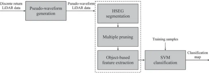
We propose a new framework for land cover classiﬁcation based on pseudo-waveforms generated from discrete return LiDAR data and object-based spatial analysis. Theﬂowchart

(3)

of the proposed framework is shown in Fig. 1. It is composed of

five steps: 1) generation of pseudo-waveforms from discrete return LiDAR data; 2) processing of pseudo-waveforms with the HSeg algorithm to subdivide the data into spatially homoge-neous regions; 3) extraction of multiple levels from the segmen-tation hierarchy by a new unsupervised pruning strategy; 4) extraction of spatial features from the regions by following a region-based approach; and 5) combining the extracted spatial features with the original pseudo-waveforms to generate final classification results. It is important to note that the processes of pseudo-waveform generation and object-based feature extrac-tion are completely unsupervised, i.e., they are based only on the information contained in the acquired LiDAR data and do not require labeled training samples. The training samples are used only in the last step of the framework to construct the classifi ca-tion model and obtain thefinal classification map. The following sections detail the methodology.

A. Pseudo-Waveform Generation

The pseudo-waveforms from LiDAR point cloud data are generated using the following method:

Algorithm 1:Pseudo-waveform generation

Input: LiDAR point cloud data, parameters , , and Output: pseudo-waveform data

1) Classify LiDAR point cloud data into ground and non-ground points.

2) Generate digital terrain model (DTM) with spatial resolu-tion ( , ) using only ground points and the natural neighbor (NN) interpolation algorithm.

3) Assign LiDAR points to corresponding pixels based on the and coordinates of the point.

4) Extract ground elevation of the points from the DTM. 5) Subtract ground elevation values from the elevation of the point (elevation above sea level) and the new value ( ) now corresponds to the elevation above ground unit.

6) For a given pixel, deﬁne 3-D voxels with the same horizontal dimension as the DTM grid structure ( , ) and vertical dimension ( ), then stack them for pseudo-wave-form generation. These voxels represent the LiDAR signal response as a function of elevation, and the LiDAR points are assigned to corresponding voxels based on the value of the points.

7) Generate the pseudo-waveform from this voxel structure by summing intensity values of all points within each voxel.

8) Normalize the pseudo-waveform data by dividing the values stored in the voxels by the number of points used to generate the corresponding pseudo-waveform. This operation is necessary to address the issue of nonuniform point density distribution, which could be generated, e.g., by acquiring the data in multiple strips with side overlap.

B. HSeg Algorithm

The HSeg algorithm combines region growing, which pro-duces spatially connected regions, with clustering, which groups similar spatially disjoint regions. The algorithm is summarized in the following, while we refer the reader to [33] for a detailed description of the method.

Algorithm 2:HSeg algorithm

Input: image, dissimilarity criterion (DC), parameter Output: segmentation hierarchy

1) Initialize segmentation by assigning each pixel to a region label. If presegmentation is provided, label each pixel accord-ingly; otherwise label each pixel as a separate region.

2) Calculate DC valuedissim_valbetween all pairs of regions. 3) Set merging thresholdthresh_valequal to the smallest value

dissim_valbetween pairs of spatially adjacent regions. A spa-tially adjacent region for a given region contains pixels located in the neighborhood (e.g., four- or eight-neighborhood) of the considered region’s pixels.

(4)

4) Merge pairs of spatially adjacent regions withdissim_val=

thresh_val.

5) If , merge pairs of nonadjacent regions with . The parameter sets the relative importance of spatially adjacent regions with respect to nonadjacent ones.

6) Stop if convergence is achieved, otherwise return to Step 2. Different measures can be used to compute DCs between the regions. Two criteria were considered in this study. We refer the reader to [35] for a detailed description of all measures implemented in the HSeg software. Theﬁrst criterion is repre-sented by the square root of band sum mean squared error (SRBSMSE) and is based on minimizing the increase of the mean squared error between the region mean image and the original data. The SRBSMSE criterion between the two regions and is deﬁned as

where is the number of pixels for region ( ), ( ) is the mean value for band and region ( ), and is the total number of bands.

The second criterion is related to the spectral angle mapper (SAM), which is deﬁned as

Merging of spatially nonadjacent regions is computationally demanding. A signiﬁcant improvement can be obtained using the RHSeg version of the algorithm, which is based on a recursive divide-and-conquer approximation of HSeg and its efﬁcient parallel implementation [33].

HSeg produces as output a hierarchy of segmentation levels. However, for practical applications, a subset of one or several segmentation levels must be selected from this hierarchy. In particular, in our context, spatial features are extracted from multiple levels. A new strategy for selecting multiple levels from the segmentation hierarchy is proposed in Section II-C.

C. Multiple Pruning

The proposed strategy extracts multiple levels from the seg-mentation hierarchy in an unsupervised way by following a pruning approach. Pruning consists of removing subtrees of the hierarchy that are homogeneous with respect to a deﬁned homogeneity criterion. In this way, theﬁnal segmentation does not represent one of the actual levels of the hierarchy, but incorporates regions selected potentially from different levels. The strategy can be thought of as automatically performing a multi-level analysis, i.e., multiple segmentation maps are ex-tracted by pruning the hierarchy in different ways.

An example of pruning applied to the segmentation hierarchy given by the HSeg algorithm is shown in Fig. 2. The segmenta-tion hierarchy is shown in Fig. 2(a) (we note that this represents

the output of the second step“HSeg segmentation”shown in Fig. 1). The top level represents the last iteration of the merging process, in which the entire image is composed of a single region (in red). Two main characteristics of the HSeg algorithm are illustrated in this example: 1) Unlike other HSeg algorithms, such as BPT, more than two regions can be merged into a single region simultaneously. For example, three different regions (yellow, orange, and cyan) at level are merged into a single region (cyan) at level ; 2) Spatially, nonadjacent regions can be merged. For example, two nonadjacent regions (red and magenta) at level are merged into a single region (red) at level . The result of the pruning is represented in Fig. 2(b), in which the segmentation hierarchy is cut, in general, at different levels. Theﬁnal segmentation map is obtained by composing all the regions, as shown in Fig. 2(c) (this coincides with the result of the third step“multiple pruning”represented in Fig. 1). Although a single pruning of the hierarchy is effectively shown in Fig. 2, multiple pruning is shown in Fig. 3, in which three different prunings of the hierarchy are performed. Different prunings are associated with different segmentation maps, which characterize the image at different levels of detail.

The pruning process can be represented as follows: Assume that regions that are distinct at a generic level of the hierarchy are merged into a single region at level . The problem consists of determining whether a cut of the hierarchy is required between level and level for the considered regions. We proposeﬁrst to characterize each region of the hierarchy in terms of local statistics. In particular, we consider second-order statistics such as standard

Fig. 2. Example of HSeg pruning: (a) hierarchical segmentation using HSeg algorithm, (b) pruning of the HSeg, and (c)ﬁnal segmentation map.

(5)

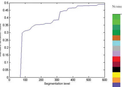
deviation. Considering a generic pixel of the image, the standard deviation value associated with the given region tends to vary across the hierarchy, as highlighted in the example shown in Fig. 4. The graph shows the standard deviation value as a function of the hierarchy level. At the beginning, when the considered region is composed only by the selected pixel, the standard deviation is equal to zero, whereas the maximum value is reached at the end, when the entire image is merged into a single region. We deﬁne as the standard deviation value associated with the region . The value is compared to the threshold value , which represents a measure of homogeneity. If , then the region is not homogeneous, so the hierarchy is cut between level and level in order to have distinct homogeneous regions . The main problem is determining the value of the threshold . We propose to select the threshold in an automatic and adaptive way. Adaptation means the threshold depends on the considered region , i.e., . This is done by considering the pixels belonging to the region and comput-ing the standard deviation in aﬁxed window of size [ , ] for each of them. The threshold value for the region is computed by applying an operator function on the standard deviation values associated with the pixels belonging to the given region. Among different operators (e.g., minimum, mean, median), the median produced the best empirical results for our data. However, calculating the threshold value directly in this way could be misleading. A pixel belonging to the spatial boundary between different objects is intrinsically characterized by a large standard deviation value if it is computed in a window. However, the pixels could belong to a very homogeneous object, which could be characterized in the segmentation hierarchy by a low standard deviation region. To alleviate this problem, for a generic pixel , we consider as not necessarily the standard deviation computed by centering the window at the pixel, but the value , where is a vector of standard deviation values calculated by centering the window at the pixel’s neighborhoods (e.g., eight-neighborhood was used in our study). We note that the standard deviation is

naturally deﬁned for single-band images. However, in our context, data are composed of several bands, so the standard deviation isﬁrst computed for each band separately, and then the mean value is considered.

Pruning of the hierarchy depends on the size [ , ] of the window used to compute the standard deviation and conse-quently the homogeneity threshold . Therefore, the multiple prunings can be obtained by varying the window size. Moreover, although the strategy has been proposed for pruning the seg-mentation hierarchy generated by the HSeg algorithm in con-junction with LiDAR data, it can be applied to any other HSeg method and data type, such as multi- or hyperspectral images. The proposed segmentation hierarchy pruning is summarized in the following:

Algorithm 3:Segmentation hierarchy pruning Input: image, segmentation hierarchy, parameter Output: segmentation map

1) Calculate for each pixel of the image the standard deviation values , using a window of size [ , ] centered at the pixel and at the pixel’s neighborhoods, respectively. Consider .

2) Consider each section of the hierarchy in which

regions that are distinct at a generic level are merged into a single region at level .

3) Calculate for the region the standard deviation value . 4) Calculate for the region the homogeneity threshold value , where is the set of standard deviation values associated with the pixels belonging to the considered region.

5) If , cut the hierarchy between levels and in order to have distinct homogeneous regions

in theﬁnal segmentation map.

Fig. 4. Example of standard deviation value associated with the belonging region for a considered pixel as a function of the segmentation level.

TABLE I

(6)

D. Object-Based Feature Extraction and Classiﬁcation

At the end of the pruning strategy, different segmentation maps are obtained, which represent the data at different levels of detail. These segmentation maps can be used to extract spatial features (e.g., textural) from the resulting regions.

In particular, we consider the occurrence and co-occurrence textural statistics [20], [41]. The occurrence statistics, orﬁrst-order features, are computed directly by considering the original values of the data. Among different measures, mean and standard deviation gave the best empirical results for the data used in these experi-ments. The co-occurrence statistics, or second-order features, are based on the grey-level co-occurrence matrix (GLCM). On the basis of this matrix, different texture descriptors can be extracted. Among the 14 descriptors proposed originally in [41], we consider six different parameters: homogeneity, contrast, dissimilarity,

entropy, second moment, and correlation. We note that the textural features are extracted independently from each band of the data.

The last step of the proposed framework consists of generating thefinal classification map. The extracted features are combined with the original pseudo-waveforms and classified. We adopt a standard SVM classifier, which has shown good performance for most remote sensing tasks [42]. We refer the reader to [43] for more details about SVM.

III. EXPERIMENTALRESULTS ANDDISCUSSION A. Experimental LiDAR and Hyperspectral Data

The dataset [44] used in this work comprises discrete return LiDAR and a hyperspectral image, acquired over the University of Houston campus. The LiDAR data were acquired on June 22,

Fig. 5. Ground reference for the University of Houston dataset.

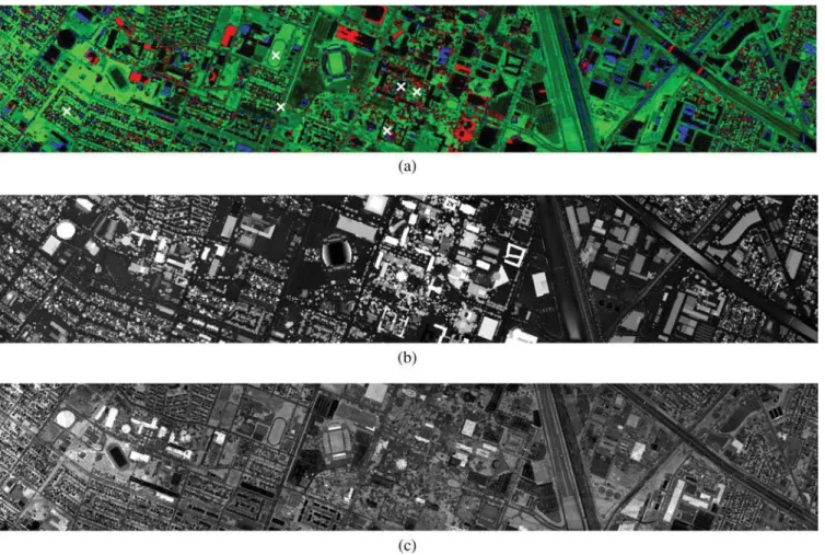
Fig. 6. False-color composite of the University of Houston dataset obtained from LiDAR data: (a) pseudo-waveform (RGB: bands 20, 10, and 15), (b) DSM, and (c) intensity.

(7)

2012, between the times 14:37:55 and 15:38:10 UTC. The data were acquired by Optech Gemini system [45] which has maxi-mum pulse repetition rate of 167 kHz and canﬂy up to 4000 m above ground level. It can record up to four returns from a return pulse. The average height of the sensor at the time of acquisition was 2000 ft above ground level, which resulted in average point density of on the ground. The hyperspectral imagery (acquired with the ITRES-CASI 1500 sensor [46]) consists of 144 spectral bands in the 380–1050 nm region and was processed (radiometric correction, attitude processing, GPS processing, geo-correction, etc.) to yield the ﬁnal geo-corrected image cube representing at-sensor spectral radiance, . Processing software provided by the manufacturer (ITRES) was utilized for this postprocessing. The hyperspectral data were acquired on June 23, 2012 between the times 17:37:10 and 17:39:50 UTC. The average height of the sensor above ground was 5500 ft, which resulted in 2.5-m spatial resolution data.

The study area represents an urban scenario, with 15 classes that are listed in Table I. The ground reference map is shown in

Fig. 5. The scene includes vegetation classes, as well as classes representing common materials in a typical urban analysis task. These classes were identified by photo-interpreting a very high resolution optical imagery of the scene acquired during the same collection.“Grass”was represented as three classes—healthy, stressed, and synthetic. Healthy and stressed grass was identified through a threshold of the normalized difference vegetation index (NDVI); synthetic grass represents artificial grass/turf. Parking lots were categorized into two distinct types—1 and 2 (one represents empty lots, and two represents lots with cars). Other classes in the dataset, as listed in Table I, are self-explanatory. From the available ground reference, 30 samples per class were selected randomly as training samples. The remaining pixels constituted the test set.

B. Experimental Setup

LiDAR points were classiﬁed into ground and nonground points using LASTools [47] with “-metro” option since the study area is located in the southeastern part of the metropolitan

Fig. 7. False-color composite of the University of Houston dataset obtained from hyperspectral data (RGB: bands 105, 61, and 40).

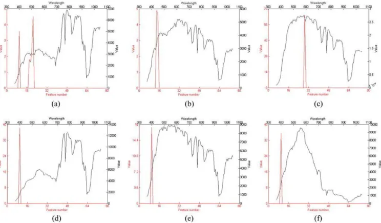
Fig. 8. Example of pseudo-waveforms from LiDAR data (in red) and spectral signatures from hyperspectral data (in black) for (a) tree, (b) residential, (c) commercial, (d) grass stressed, (e) road, and (f) water classes.

(8)

city, Houston. The same grid structure of the hyperspectral data with 2.5-m spatial resolution was adopted in generating pseudo-waveform data from the discrete return LiDAR data. The DTM with the same 2.5-m grid structure was generated using only ground points and the NN interpolation algorithm. For a given pixel, 80 voxels with the same horizontal dimension as the grid ( , ) and 1-m vertical resolution ( ) were created. The voxels were designated such that the 1) bottom, 2) 10th, and 3) top voxel corresponds to the LiDAR signal at 1) 9 m below the ground elevation, 2) ground elevation, and 3) 70 m above the ground elevation of the corresponding pixel location, and each layer of the voxel struc-ture can be interpreted as a band that represents LiDAR signal response at the corresponding elevation above the ground. The DSM and intensity images were also generated from the original LiDAR point cloud data to compare the results obtained using these data to those obtained using pseudo-waveforms. The DSM was generated using the same 2.5-m grid structure by calculating the maximum elevation of the points within every pixel. The intensity image was generated from the point cloud data byﬁrst summing all intensity value of points assigned to the pixel and then by dividing the sum by the number of points of the pixel. LiDAR products and hyperspectral image are shown in Figs. 6 and 7, respectively. Moreover, for some speciﬁc pixels of the images, represented with crosses and related to different classes, we show in Fig. 8 the pseudo-waveform and

the corresponding spectral signature: 1) Tree, 2) Residential, 3)Commercial, 4)Grass stressed, 5)Road, and 6)Water. These examples illustrate that the structural differences represented in pseudo-waveforms can be utilized in the classiﬁcation process. We especially note that two classes, i.e.,Residentialand Com-mercial, are spectrally similar but have different structural characteristics.

The HSeg algorithm was applied to pseudo-waveform, DSM, intensity, and hyperspectral data by adopting a four-neighborhood connectivity. In terms of DC, the pseudo-waveform and hyper-spectral data were processed using the SAM criterion [48] (we note that in this way all available bands are considered by the algorithm). However, since this criterion is not meaningful for single-band images, the SRBSMSE measure was adopted for DSM and intensity data. For all cases, the parameter , which sets the importance of nonadjacent regions in the region growing process, wasﬁxed to 0.1.

The strategy proposed for segmentation hierarchy pruning requires setting two main parameters. The number of prunings of the hierarchy, i.e., the number of segmentation maps ex-tracted from the HSeg result, is an input. For all the cases, we considered three different prunings. For each pruning, it is necessary to deﬁne the parameter , which is related to the size of the window used for computing the homogeneity threshold. Windows with size [3, 3], [5, 5], and [7, 7] were considered.

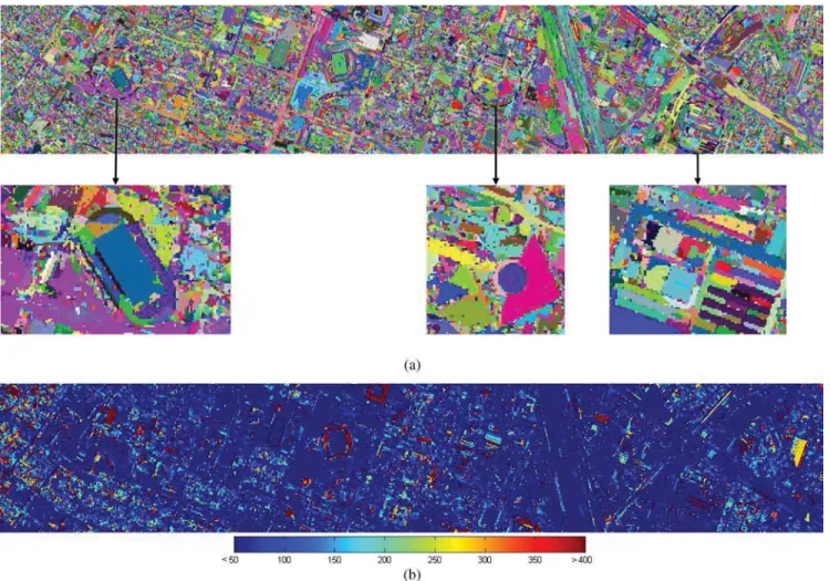
Fig. 9. Result of the proposed pruning strategy on the segmentation hierarchy generated by the HSeg algorithm on the pseudo-waveforms data: (a) segmentation map and (b) pruning level map.

(9)

The features were normalized in the range [0, 1]. SVM classification was accomplished using a Gaussian RBF kernel. The SVM hyper-parameters were selected by a fivefold cross validation applied on the training set. The and parameters were selected in the range [ , ] and [ , ], respectively. The LIBSVM library [49] was used to solve the SVM classifi -cation problem. Classification performances were evaluated by different measures: 1) the overall accuracy (OA), 2) the Kappa statistic [50], 3) the classification accuracies obtained for indi-vidual classes, and 4) the average accuracy (AA).

The experimental analysis can be subdivided into two main parts. In the first part, we compared the classification results obtained by considering the proposed framework, in which pseudo-waveforms were used, with the results obtained by adopting basic LiDAR products, such as DSM and intensity. Moreover, the results given by the proposed object-based feature extraction were compared to those given by a more traditional window-based approach. In this case, for a fair comparison, the same window sizes were considered. In the second part, the analysis of hyperspectral and LiDAR data was conducted to demonstrate complementary of the two data sources for perform-ing land cover classification.

C. Experimental Results and Discussion

Before presenting the results in terms of classiﬁcation accura-cies, we evaluate the proposed pruning strategy in a qualitative way. We show in Fig. 9 the result obtained by applying the pruning strategy on the segmentation hierarchy generated by the HSeg algorithm on the pseudo-waveform data. In this case, the parameter [ , ] necessary for estimating the homogeneity threshold was set to [3, 3]. Therefore, the resulting segmentation map (random colors have been assigned to different regions), shown in Fig. 9(a),

represents aﬁner level of detail of the image. A good segmentation result has been obtained, as highlighted by the zoomed parts of the image. Moreover, we show in Fig. 9(b), the corresponding pruning level map. The color of the map refers to the level in which the segmentation hierarchy was cut for the considered region. For example, blue and red regions were extracted from theﬁrst and last levels of the hierarchy, respectively. It is clear how the segmentation map was effectively obtained by extracting different regions from different levels of the hierarchy.

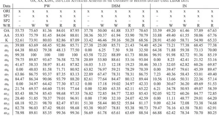
In thefirst part of the experiments, classification accuracies based on the proposed framework by adopting pseudo-waveforms were compared with the results obtained by considering basic LiDAR products, such as DSM and intensity (IN). The results are summarized in Table II. In general, the proposed framework in conjunction with pseudo-waveform data greatly improved the classification accuracies in comparison with the other cases (DSM and intensity). When only the original (ORI) data were considered, the pseudo-waveform gave , and OA was equal to 37.78% and 33.59% for the DSM and intensity cases, respectively. Higher accuracies were exhibited by pseudo-wa-veforms also when spatial features were added to the original data. Comparing region-based (R) and window-based (W) feature extraction approaches, better results were obtained using the proposed approach. For example, by adding the

first-order textural features (SP1), the OA for the pseudo-waveform case was equal to 84.01% and 75.65% for the region-based and the window-based approaches, respectively. Similar improvements were also verified by considering DSM ( and 50.00%, respectively) and intensity ( and 49.20%, respectively) data. These results validated the effectiveness of the proposed region-based feature extraction strategy. Similar considerations can also be per-formed by adding the second-order textural features (SP2), in which a further improvement of the accuracies was verified.

TABLE II

(10)

Considering the pseudo-waveform (DSM and intensity) data, OA was equal to 87.95% (70.65% and 67.63%) and 81.36% (61.88% and 61.46%) for the region-based and the window-based approaches, respectively. The best result ( ) was obtained when we considered bothfirst- and second-order textural features extracted from pseudo-waveform data by following a region-based approach. This indicates that utilizing pseudo-waveform data generated from the raw LiDAR point cloud has really significantly improved the overall classifi ca-tion accuracy for these data.

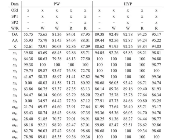
In the second part of the experimental analysis, we investi-gated the classification accuracies obtained by applying the proposed framework to the hyperspectral data. The results are shown in Table III. For hyperspectral data, we observed a classification accuracy pattern similar to that described previ-ously for LiDAR data. In particular, also for hyperspectral data, classification accuracies were improved as we added the textural features to the original spectral signatures. Moreover, better results were obtained by extracting features by following a region-based approach. The best result was verified when both

ﬁrst- and second-order features were considered (OA equals to 95.17% and 87.95% for hyperspectral and pseudo-waveform data, respectively). Analyzing in greater detail the class accura-cies, six classes ( , , , , , and ) yielded weak classiﬁcation results when only the original pseudo-waveform data were considered ( : 39.88%, : 41.67%, : 0.00%, : 0.00%, : 21.74%, and : 28.40%). However, the inclusion of textural features improved the accuracies for these weak classes ( : 45.83%, : 46.15%, : 80.92%, : 87.12%, : 55.9%, and : 68.51%). Although the OA

for the hyperspectral data was higher than that obtained for the pseudo-waveform data, when both ﬁrst- and second-order textural features were utilized in addition to the original data, three classes ( , , and ) yielded better accuracies for the pseudo-waveform case. These observations indicate that these classes (Residential,Commercial, andRailway) can be better separated using the structural information provided by the pseudo-waveform data. These observations suggest how a fur-ther improvement of the overall classiﬁcation accuracy can be obtained by fusing LiDAR and hyperspectral data.

IV. CONCLUSION

In this work, we have proposed a new framework for land cover classification using discrete return LiDAR data. In partic-ular, pseudo-waveforms have been generated from the discrete return LiDAR data and processed by the HSeg segmentation algorithm. A new strategy for multiple pruning of the segmenta-tion hierarchy has been proposed in order to extract spatial features from homogeneous regions by following a region-based approach. Finally, the extracted features have been combined with the original pseudo-waveforms data and classified using SVM classification.

Novelties and key points of the proposed framework can be summarized as follows: 1) the land cover classiﬁcation problem has been addressed in an innovative way by incorporating pseudo-waveforms and object-based spatial analysis; 2) the effectiveness of the state-of-the-art HSeg algorithm has been validated on LiDAR data, whereas previous research has been conducted on multi- and hyperspectral data; 3) the HSeg

TABLE III

(11)

algorithm has been used as a preprocessing step for object-based feature extraction, while it was used for different purposes in the previous works (e.g., as postprocessing for spatial regularization [33], [36] or as preprocessing for ground reference design [51], [52]); and 4) the pruning of the segmentation hierarchy has been addressed by a new unsupervised multi-level strategy.

The proposed framework has been validated experimentally on a dataset acquired in an urban area at the University of Houston. The experimental results reveal that the proposed framework, in conjunction with pseudo-waveform data, has given an improvement of the classification accuracies with respect to the cases in which basic LiDAR products, such as DSM or intensity, have been used. Moreover, the proposed region-based feature extraction process has been able to give better results in comparison with a more traditional window-based approach. Finally, although the best accuracies have been obtained, in general, by considering the hyperspectral data, the use of pseudo-waveforms has shown a promising performance. In particular, some classes have been classified better using LiDAR data than with the hyperspectral data. This suggests classification accuracies may be further improved by fusing the LiDAR and hyperspectral data. Future research will be con-ducted to fully exploit synergistic effects between the LiDAR and hyperspectral data for performing land cover classification.

ACKNOWLEDGMENTS

The authors would like to thank the Hyperspectral Image Analysis group and the NSF Funded Center for Airborne Laser Mapping (NCALM) at the University of Houston for providing the datasets used in this study, and the IEEE GRSS Data Fusion Technical Committee for organizing the 2013 Data Fusion Contest.

REFERENCES

[1] J. A. Benediktsson, M. Pesaresi, and K. Arnason, “Classiﬁcation and feature extraction for remote sensing images from urban areas based on morphological transformations,” IEEE Trans. Geosci. Remote Sens., vol. 41, no. 9, pp. 1940–1949, Sep. 2003.

[2] A. K. Shackelford and C. H. Davis,“A hierarchical fuzzy classiﬁcation approach for high-resolution multispectral data over urban areas,”IEEE Trans. Geosci. Remote Sens., vol. 41, no. 9, pp. 1920–1932, Sep. 2003. [3] F. Dell’Acqua, P. Gamba, A. Ferrari, and J. A. Palmason,“Exploiting spectral

and spatial information in hyperspectral urban data with high resolution,” IEEE Geosci. Remote Sens. Lett., vol. 1, no. 4, pp. 322–326, Oct. 2004. [4] J. A. Benediktsson, J. A. Palmason, and J. R. Sveinsson,“Classiﬁcation of

hyperspectral data from urban areas based on extended morphological proﬁles,”IEEE Trans. Geosci. Remote Sens., vol. 43, no. 3, pp. 480–491, Mar. 2005.

[5] E. W. Bork and J. G. Su,“Integrating LiDAR data and multispectral imagery for enhanced classiﬁcation of rangeland vegetation: A meta analysis,” Remote Sens. Environ., vol. 111, no. 1, pp. 11–24, Nov. 2007.

[6] M. Dalponte, L. Bruzzone, and D. Gianelle,“Fusion of hyperspectral and LiDAR remote sensing data for classiﬁcation of complex forest areas,” IEEE Trans. Geosci. Remote Sens., vol. 46, no. 5, pp. 1416–1427, May 2008.

[7] A. Alonso-Gonzalez, S. Valero, J. Chanussot, C. Lopez-Martinez, and P. Salembier,“Processing multidimensional SAR and hyperspectral images with binary partition tree,” Proc. IEEE, vol. 101, no. 3, pp. 723–747, Mar. 2013.

[8] J. Jung and M. M. Crawford,“Extraction of features from LiDAR waveform data for characterizing forest structure,”IEEE Geosci. Remote Sens. Lett., vol. 9, no. 3, pp. 492–496, May 2012.

[9] B. K. Pekin, J. Jung, L. J. Villanueva-Rivera, B. C. Pijanowski, and J. A. Ahumada,“Modeling acoustic diversity using soundscape recordings and LiDAR-derived metrics of vertical forest structure in a neotropical rainforest,”Landsc. Ecol., vol. 27, no. 10, pp. 1513–1522, Dec. 2012.

[10] J. Jung, B. K. Pekin, and B. C. Pijanowski,“Mapping open space in an old-growth, secondary-growth, and selectively-logged tropical rainforest using discrete return LiDAR,”IEEE J. Sel. Topics Appl. Earth Observ. Remote Sens., vol. 6, no. 6, pp. 2453–2461, Dec. 2013.

[11] A. S. Antonarakis, K. S. Richards, and J. Brasington,“Object-based land cover classiﬁcation using airborne LiDAR,” Remote Sens. Environ., vol. 112, no. 6, pp. 2988–2998, Jun. 2008.

[12] A. P. Charaniya, R. Manduchi, and S. K. Lodha,“Supervised parametric classiﬁcation of aerial LiDAR data,”inProc. CVPRW’04,Jun. 2004. [13] J. H. Song, S. H. Han, K. Y. Yu, and Y. I. Kim,“Assessing the possibility of

land cover classiﬁcation using LiDAR intensity data,”Int. Arch. Photo-gram. Remote Sens. Spatial Inf. Sci., vol. 34, no. 3/B, pp. 259–262, 2002. [14] J. D. Muss, D. J. Mladenoff, and P. A. Townsend,“A pseudo-waveform technique to assess forest structure using discrete LiDAR data,”Remote Sens. Environ., vol. 115, no. 3, pp. 824–835, Mar. 2011.

[15] D. A. Landgrebe,Signal Theory Methods in Multispectral Remote Sensing, New York, NY, USA: Wiley, 2003.

[16] A. Plaza, A. Benediktsson, J. Boardman, J. Brazile, L. Bruzzone, G. Camps-Valls, J. Chanussot, M. Fauvel, P. Gamba, J. A. Gualtieri, M. Marconcini, J. C. Tilton, and G. Trianni,“Recent advances in techniques for hyperspectral image processing,”Remote Sens. Environ., vol. 113, no. 1, pp. S110–S122, Sep. 2009.

[17] M. Fauvel, Y. Tarabalka, J. A. Benediktsson, J. Chanussot, and J. C. Tilton, “Advances in spectral-spatial classiﬁcation of hyperspectral images,”in Proc. IEEE, vol. 101, no. 3, pp. 652–675, Mar. 2013.

[18] R. L. Kettig and D. A. Landgrebe,“Classiﬁcation of multispectral image data by extraction and classiﬁcation of homogeneous objects,”IEEE Trans. Geosci. Electron., vol. 14, no. 1, pp. 19–26, Jan. 1976.

[19] Q. Jackson and D. A. Landgrebe,“Adaptive Bayesian contextual classiﬁ -cation based on Markov randomﬁelds,”IEEE Trans. Geosci. Remote Sens., vol. 40, no. 11, pp. 2454–2463, Nov. 2002.

[20] A. Baraldi and F. Parmiggiani, “An investigation of the textural characteristics associated with gray level co-occurrence matrix statistical parameters,” IEEE Trans. Geosci. Remote Sens., vol. 33, no. 2, pp. 293–304, Mar. 1995.

[21] B. Kartikeyan, A. Sarkar, and K. L. Majumder,“A segmentation approach to classiﬁcation of remote sensing imagery,”Int. J. Remote Sens., vol. 19, no. 9, pp. 1695–1709, 1998.

[22] G. Camps-Valls, L. Gomez-Chova, J. Munoz-Mari, J. Vila-Frances, and J. Calpe-Maravilla, “Composite kernel for hyperspectral image classiﬁcation,” IEEE Geosci. Remote Sens. Lett., vol. 3, no. 1, pp. 93–97, Jan. 2006.

[23] M. Fauvel, J. Chanussot, and J. A. Benediktsson,“A spatial-spectral kernel-based approach for the classiﬁcation of remote-sensing images,”Pattern Recogn., vol. 45, no. 1, pp. 381–392, Jan. 2012.

[24] R. C. Gonzalez and R. E. Woods,Digital Image Processing, 2nd ed., Englewood Cliffs, NJ, USA: Prentice-Hall, 2002.

[25] A. K. Shackelford and C. H. Davis,“A combined fuzzy pixel-based and object-based approach for classiﬁcation of high-resolution multispectral data over urban area,”IEEE Trans. Geosci. Remote Sens., vol. 41, no. 10, pp. 2354–2363, Oct. 2003.

[26] C. A. Bouman and M. Shapiro,“A multiscale randomﬁeld model for Bayesian image segmentation,”IEEE Trans. Image Process., vol. 3, no. 2, pp. 162–177, Mar. 1994.

[27] E. Binaghi, I. Gallo, and M. Pepe,“A cognitive pyramidal for contextual classiﬁcation of remote sensing images,” IEEE Trans. Geosci. Remote Sens., vol. 41, no. 12, pp. 2906–2922, Dec. 2003.

[28] F. Paciﬁci, M. Chini, and W. J. Emery,“A neural network approach using multi-scale textural metrics from very high-resolution panchromatic imag-ery for urban land-use classiﬁcation,”Remote Sens. Environ., vol. 113, no. 6, pp. 1276–1292, Jun. 2009.

[29] H. G. Akçay and S. Aksoy,“Automatic detection of geospatial objects using multiple hierarchical segmentations,”IEEE Trans. Geosci. Remote Sens., vol. 46, no. 7, pp. 2097–2111, Jul. 2008.

[30] R. Brennan and T. L. Webster,“Object-oriented land cover classiﬁcation of LiDAR-derived surfaces,” Can. J. Remote Sens., vol. 32, no. 2, pp. 162–172, 2006.

[31] G. Miliaresis and N. Kokkas,“Segmentation and object-based classiﬁcation for the extraction of the building class from LiDAR DEMs,” Comput. Geosci., vol. 33, no. 8, pp. 1076–1087, Aug. 2007.

[32] F. Rottensteiner and C. Briese,“A new method for building extraction in urban areas from high-resolution LiDAR data,” Int. Arch. Photogram. Remote Sens. Spatial Inf. Sci., vol. 34, pp. 295–301, 2002.

[33] J. C. Tilton, Y. Tarabalka, P. M. Montesano, and E. Gofman,“Best merge region-growing segmentation with integrated nonadjacent region object aggregation,” IEEE Trans. Geosci. Remote Sens., vol. 50, no. 11, pp. 4454–4467, Nov. 2012.

[34] J. M. Beaulieau and M. Goldberg,“Hierarchy in picture segmentation: A stepwise optimization approach,”IEEE Trans. Pattern Anal. Mach. Intell., vol. 11, no. 2, pp. 150–163, Feb. 1989.

(12)

[35] J. C. Tilton (Nov. 2012). RHSeg user’s manual: Including HSWO, HSeg, HSegExtract, HSegReader and HSegViewer, version 1.59. [36] Y. Tarabalka, J. A. Benediktsson, J. Chanussot, and J. C. Tilton,“Multiple

spectral-spatial classiﬁcation approach for hyperspectral data,”IEEE Trans. Geosci. Remote Sens., vol. 48, no. 11, pp. 4122–4132, Nov. 2010. [37] A. J. Plaza and J. Tilton,“Automated selection of results in hierarchical

segmentation of remotely sensed hyperspectral images,”Proc. IGARSS’05, vol. 7, pp. 4946–4949, Jul. 2005.

[38] Y. Tarabalka, J. C. Tilton, J. A. Benediktsson, and J. Chanussot,“A marker-based approach for the automated selection of a single segmentation from a hierarchical set of image segmentation,”IEEE J. Sel. Topics Appl. Earth Observ. Remote Sens., vol. 5, no. 1, pp. 262–272, Feb. 2012.

[39] P. Salembier and L. Garrido,“Binary partition tree as an efﬁcient represen-tation for image processing, segmenrepresen-tation and information retrieval,”IEEE Trans. Image Process., vol. 9, no. 4, pp. 561–576, Apr. 2000.

[40] S. Valero, P. Salembier, and J. Chanussot,“Hyperspectral image represen-tation and processing with binary partition trees,” IEEE Trans. Image Process., vol. 22, no. 4, pp. 1430–1443, Apr. 2013.

[41] R. M. Haralick, K. Shanmuga, and I. H. Dinstein,“Textural features for image classiﬁcation,” IEEE Trans. Syst. Man Cybern., vol. 3, no. 6, pp. 610–621, Nov. 1973.

[42] F. Melgani and L. Bruzzone, “Classiﬁcation of hyperspectral remote sensing images with support vector machines,” IEEE Trans. Geosci. Remote Sens., vol. 42, no. 8, pp. 1778–1790, Aug. 2004.

[43] V. N. Vapnik,Statistical Learning Theory, New York, NY, USA: Wiley, 1998. [44] 2013 IEEE GRSS Data Fusion Contest, [Online]. Available: http://www.

grss-ieee.org/community/technical-committees/data-fusion/. [45] [Online]. Available: http://www.optech.ca/gemini.htm.

[46] ITRES Research Ltd., [Online]. Available: http://www.itres.com/products/ imagers/casi1500/.

[47] LAS Tools, [Online]. Available: http://www.cs.unc.edu/~isenburg/ lastools/.

[48] F. A. Kruse, A. B. Lefkoff, J. W. Boardman, K. B. Heidebrecht, A. T. Shapiro, P. J. Barloon, and A. F. H. Goetz,“The spectral image processing system (SIPS)—Interactive visualization and analysis of imaging spectrometer data,” Remote Sens. Environ., vol. 44, no. 2/3, pp. 145–163, May/Jun. 1993. [49] C. Chang and C. Lin, LIBSVM–A library for support vector machine, 2008

[Online]. Available: http://www.csie.ntu.edu.tw/~cjlin/libsvm.

[50] J. Cohen,“A coefﬁcient of agreement for nominal scales,”Educ. Psychol. Meas., vol. 20, no. 1, pp. 37–46, 1960.

[51] E. Pasolli, F. Melgani, N. Alajlan, and N. Conci,“Optical image classiﬁ ca-tion: A ground-truth design framework,”IEEE Trans. Geosci. Remote Sens., vol. 51, no. 6, pp. 3580–3597, Jun. 2013.

[52] J. Tilton, E. B. de Colstoun, R. E. Wolfe, T. Bin, and H. Chengquan, “Generating ground reference data for a global impervious surface survey,” inProc. IGARSS’12, vol. 1, pp. 5993–5996, Jul. 2012.

Jinha Jung(S’08) received the B.S. degree in Civil, Urban, and Geosystem Engineering Department from the Seoul National University, Seoul, Korea, in 2003, and the M.S. degree from the same department in 2005. He received the Ph.D. degree in Geomatics Department of the School of Civil Engineering from the Purdue University, West Lafayette, IN, USA, in 2011.

He worked as a Postdoctoral Research Associate at the Institute for Environmental Science and Policy of the University of Illinois at Chicago, IL, USA, and currently works as a Postdoctoral Research Associate in the School of Civil Engineering of the Purdue University, West Lafayette, IN, USA. His main research interest is the advanced LiDAR data analysis for interdisciplinary research leveraging his specialties in remote sensing and geospatial science.

Edoardo Pasolli (S’08–M’13) received the M.Sc. degree in telecommunications engineering and the Ph.D. degree in information and communication tech-nologies from the University of Trento, Trento, Italy, in 2008 and 2011, respectively.

He was a Postdoctoral Fellow with the Intelligent Information Processing Laboratory, Department of Information Engineering and Computer Science, Uni-versity of Trento, Trento, Italy, from December 2011 to September 2012, and with the Computational and Information Sciences and Technology Ofﬁce, NASA

Goddard Space Flight Center, Greenbelt, MD, USA, from October 2012 to October 2013. He is currently a Postdoctoral Fellow with the School of Civil Engineering, Purdue University, West Lafayette, IN, USA. His current research interests include processing and recognition techniques applied to remote sensing images and biomedical signals.

Saurabh Prasad (S’05–M’09) received the B.S. degree in electrical engineering from Jamia Millia Islamia, New Delhi, India, in 2003, the M.S. degree in electrical engineering from Old Dominion University, Norfolk, VA, USA, in 2005, and the Ph.D. degree in electrical engineering from Mississippi State Univer-sity, Starkville, MS, USA, in 2008.

He is currently an Assistant Professor in the Electrical and Computer Engineering Department at the University of Houston (UH), Houston, TX, USA. He leads the Hyperspectral Image Analysis group at UH, and is also afﬁliated with UH’s Geosensing Systems Engineering Research Center at UH. His research interests include signal processing and machine learning for optical and microwave remote sensing, and biomedical applications.

James C. Tilton (S’79–M’81–SM’94) received the B.A. degrees in electronic engineering, environmental science and engineering, and anthropology and the M.E.E. degree in electrical engineering from Rice University, Houston, TX, USA, in 1976. He also received the M.S. degree in optical sciences from the University of Arizona, Tucson, AZ, USA, in 1978 and the Ph.D. degree in electrical engineering from Purdue University, West Lafayette, IN, USA, in 1981.

He is currently a Computer Engineer with the Computational and Information Sciences and Technol-ogy Ofﬁce (CISTO) of the Science and Exploration Directorate at the NASA Goddard Space Flight Center, Greenbelt, MD, USA. As a member of CISTO, he is responsible for designing and developing computer software tools for space and earth science image analysis and encouraging the use of these computer tools through interactions with space and Earth scientists. His software development has resulted in three patents. He has held similar positions at NASA Goddard, since 1985.

Dr. Tilton is a senior member of the IEEE Geoscience and Remote Sensing Society (GRSS). From 1992 to 1996, he served as a member of the IEEE GRSS Administrative Committee. Since 1996, he has served as an Associate Editor for the IEEE TRANSACTIONS ONGEOSCIENCE ANDREMOTESENSING.

Melba M. Crawford (M’90–SM’05–F’08) received the B.S. and M.S. degrees in civil engineering from the University of Illinois at Urbana-Champaign, Urbana, IL, USA and the Ph.D. degree in systems engineering from the Ohio State University, Columbus, OH, USA.

She was a Faculty Member with the University of Texas, Austin, TX, USA, from 1990 to 2005, where she founded an interdisciplinary research and applications development program in space-based and airborne remote sensing. She is currently with Purdue University, West Lafayette, IN, USA, where she is the Director of the Laboratory for Applications of Remote Sensing and the Associate Dean of Engineering for Research. She has served as a member of the NASA Earth System Science and Applications Advisory Committee and was a member of the NASA EO-1 Science Validation team for the Advanced Land Imager and Hyperion. Her research interests focus on hyperspectral and LiDAR sensing, data fusion for multi-sensory problems, manifold learning, and knowledge transfer in data mining.

Dr. Crawford was a Jefferson Senior Science Fellow of the U.S. Department of State in 2004–2005 and continues to serve in an advisory capacity. She is the current President of the IEEE GEOSCIENCE ANDREMOTESENSINGSOCIETY.