Construction of Jakarta Land Use/Land Cover
Dataset Using Classification Method
Tjeng Wawan Cenggoro
School of Computer ScienceBina Nusantara University Jakarta, Indonesia
e-mail: [email protected]
Sani M. Isa
Master of Information Technology Bina Nusantara University
Jakarta, Indonesia e-mail: [email protected]
Gede Putra Kusuma
Master of Information TechnologyBina Nusantara University Jakarta, Indonesia e-mail: [email protected]
Abstract—The field of remote sensing has drawn a lot of attention recently. However, collecting necessary ground truth data for research in this field requires a lot of effort. There-fore, this paper presents a method for constructing estimated ground truth data using classification. This method reduces the workload in collecting remote sensing ground truth data. The contribution of this paper is to prepare and provide estimated Land Cover/Land Use (LULC) ground truth data of Jakarta area using the proposed method. The estimated ground truth data then can be used along with remote sensing image of Jakarta area to form dataset, which can be used for remote sensing research.
For the estimated ground truth data to be reliable, the employed classification model have to achieve a reasonably good result. This research compares several algorithms to find the classification model with the best result for this case. The experimental result shows that Neural Network with single hidden layer of 30 neurons achieves best test accuracy of 75.41%. The method of this paper has been successfully implemented to construct LULC dataset of Jakarta area.
Index Terms—remote sensing, land use, land cover, dataset, classification.
I. INTRODUCTION
Remote sensing has become a popular research topic. This popularity came from its widespread applications in different research fields such as computer science [1]–[3], environmen-tal science [4]–[6], social science [7]–[10], and agriculture [11]–[13]. Moreover, the easiness in accessing the remotely sensed image also contribute to its popularity. While other research field often has a difficulty in gathering necessary data, remotely sensed image across the world can be acquired easily and freely. One of the source where the images can be acquired for free is from United States Geological Survey (USGS) website [14].
Eventhough the images can be easily acquired, obtaining the ground truth of the images is difficult. Traditionally, in order to obtain ground truth data, a direct land survey is necessary. However, this approach requires expensive cost, laborious works, and great amount of time. Alternative approach is to do land survey via high resolution image. While this method requires less time than direct land survey, it still requires expensive cost to obtain the high resolution images. There is also another method utilizing clustering algorithm to generate estimated ground truth. However, the generated estimated ground truth is not reliable due to the nature of the algorithm.
The limitation of the existing methods leads to the scarcity of available ground truth data. The lack of easily accessible ground truth data hinders the advancement of remote sensing researches, especially in LULC modeling.
Because of the importance in having enough LULC data for promoting a good LULC research, this paper attempts to expand the data that can be used by exploiting available LULC ground truth. This is done by performing classification using existing ground truth from certain period of time as training data. The resulting classification model then applied to classify unlabeled remote sensing images from other period. By using this approach, it is possible to acquire more LULC data cheaper and faster than performing direct land survey.
Despite of its effectiveness, it should be noticed that this approach rely heavily on the result of the classification model. In other words, to obtain a reliable dataset using this approach, the selected classification model should produce a good result. Therefore, this paper also aims to find classification algorithm that is accurate enough for the purpose of this paper.
II. CLASSIFICATIONALGORITHMS
To find the best classification model, performance of several algorithms are compared. These algorithms are sourced from Rapidminer software (formerly known as Yale) [15]. There are four algorithms to be compared: k Nearest Neighbor (k-NN), Logistic regression, Support Vector Machine (SVM), and Neural Network (NN). For each of the classification model, there is no regularization technique applied.
The first algorithm, k-NN, is a classification algorithm that works by considering classes ofknumber of closest neighbor. The predicted class of a certain data point is decided by voting among k number of closest data points. k-NN is based on assumption that points with close differences in their attributes value tend to fall in a same class [16]. The differences can be calculated by using measurement such as proximity, correlation, jaccard similarity, and cosine similarity [17]. For example of k-NN using proximity, consider two data point with n attributes X(x1, x2, ..., xn) and Y(y1, y2, ..., yn). To
calculate their proximity, euclidean distance measurement can be employed. Eq. 1 shows the formula of euclidean distance, whereddenotes the proximity between point X andY.
d=p(x1−y1)2+ (x2−y2)2+...+ (xn−yn)2 (1) The second algorithm, logistic regression, is a regression method that applied to binary data. It has a similar process to linear regression, except for its model and assumption [18]. Not only it receives binary input, logistic regression model also produces output in binary form. To describe the logistic regression process, consider a linear regression process over a vector x∈ Rn. The output y then calculated using eq. 2, whereβifromi= 0tonare adjustable parameters for fitting the equation to the data distribution. It can be seen that in eq. 2, yalso is a member ofRn, which is not in the form of binary. Thus, logistic regression needs to use different equation to produce binary output. Logistic regression use logistic function as shown in eq. 3 to map the output to binary form,y∈ {0,1}. Y =β0+ Σni=1βixi (2)
y= e
β0+Σni=1βixi 1 +eβ0+Σni=1βixi
(3) The third algorithm, SVM, was introduced by Cortes et al. in 1995 [19]. SVM is a classification algorithm that separates data to binary label,[−1,1]. The basic idea of SVM is to find an optimal separator (hyperplane) between the binary label. The hyperplane can be a linear, polynomial, or radial basis function. For instance, consider an SVM model with linear hyperplane. The formula of the optimal hyperplane is written as eq. 4. Here in eq. 4, b0 denotes the intercept term of the
equation. w0 calculated as linear combination of closest data
points (support v) to the hyperplane from both binary label. These closest data points also known as support vector. The calculation ofw0is described by eq. 5. The goal of SVM is to
find a hyperplane that maximize its margin to support vectors. This margin is calculated as eq. 6. After finding the optimal hyperplane, the SVM model can predict an input data label by calculating the result of decision function, denoted in eq. 7.
b0+w0z= 0 (4) w0= Σi∈{support vector}αizi (5) ρ(w0, b0) = 2 |w0| (6) I(z) =b0+w0z (7)
The last algorithm, NN, is an algorithm which is modeled after how biological neurons processing information. NN is a non-linear model that map input vector z ∈ Rn to a certain output vector [20]. NN is built from numbers of interconnected computing units, named as neuron. Each neurons typically calculates linear combination of its input vector as shown in eq. 8. The net outputynetis then applied to a specific transfer functionfAN to produce the output of neuron as shown in 9.
For the activation function, NN typically use sigmoid function, f(x) = 1
1+e−x. To create a model of NN, neurons are arranged to specific architecture, which a neuron may take other neuron output as its input.
ynet=v0+ Σni=1zivi (8)
y=fAN(ynet) (9)
III. METHODOLOGY
The methodology of this research is illustrated in fig. 1. It can be divided into three phases: Data acquisition and pre-processing, classification model training, and estimated ground truth data construction. In the first phase, the necessary data are collected and pre-processed so that they are ready to be used. The second phase is performed to train different classification models and compare their performances. In the last phase, the best classification model is picked and applied to the unlabeled remote sensing images.
Fig. 1: Workflow of Research. IV. MATERIALS ANDEXPERIMENTALSETUP
A. Study Area
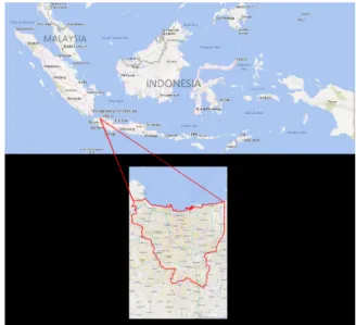
The study area in this research covers the area of Jakarta City, excluding its small islands area calledKepulauan Seribu. This Region of Interest (RoI) span from 6◦4’38” to 6◦22’21” in latitude and 106◦40’11” to 106◦59’1” in longitude; It is shown in fig. 2. Jakarta is the capital city of Indonesia, with its LULC mostly are urban areas. There are also a considerable area of agriculture and non-agriculture vegetation.
B. Remote Sensing Images and Pre-Processing
The remote sensing images used for classification are ac-quired by Landsat 7 satellite with WRS-2 path 122 and row 64; which contains the whole area of Jakarta. The images were downloaded from USGS website [14] at December 5, 2015. For the training data, images from year 2000 is employed. It is chosen based on the available ground truth data provided by
Badan Informasi Geospasial(BIG), the Indonesian Geospatial Information Agency. As for the unlabeled images which estimated ground truth will be constructed, are taken from the images of recent four years (2012 - 2015).
Before the images can be used for classification process, they must undergo several pre-processing steps. Firstly, the atmospheric correction is performed on the image. The cor-rection is carried out using semi classification plugin in QGIS software [21]. On the other hand, the geometric correction is not necessary because the features used fot classification are only extracted from a single image. Afterward, the image is cropped to the RoI defined in section IV-A. The last step is to detect and remove areas that are covered by clouds and shadow of clouds. The cloud detection is performed using algorithm developed by Zhu et al. [22], which is an improvement of the previous algorithm [23].
After pre-processing steps, the image is translated into feature vectors to be used in classification process. The feature vectors are formed by using 6 bands out of 8 bands from Landsat 7 image. The utilized bands are Band 1 to 5 and Band 7. Band 6 and Band 8 are left out due to their different resolution from other bands.
C. Ground Truth Data
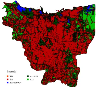
The ground truth data is obtained from Badan Informasi Geospasial (BIG) website [24] at December 5, 2015. This ground truth is mapped by BIG in year 2000 with the scale of 1:25,000. This ground truth is in the form of shapefile, which is a vector format image. Thus, each of the class labels are defined through areas. It makes them not directly tied to the image pixels. The illustration of the acquired ground truth data is shown in fig. 3
There are thirteen classes in the ground truth data, as defined by BIG, for the corresponding RoI. These classes are listed in table I. To scale the classes scope to this research, these thirteen classes are grouped into several major classes according to Indonesian National Standard of Land Cover Classification [25]. These major classes are then associated to classes in dichotomous phase of United Nation Food and Agriculture Association Land Cover Classification System (UNFAO-LCCS) as shown in table II. As for the class dis-tribution the ground truth is shown in table III.
D. Training, Validation, and Test Samples Distribution
It is necessary to validate and test different configurations of classification methods using separate datasets to find the best performing method. In concern to this needs, a simple split validation is not enough. Therefore, the whole dataset used in this research is divided into three set. The first set
Fig. 3: Illustration of ground truth data.
TABLE III: Class Distribution of the Available Ground Truth No. UNFAO-LCCS Code Number of Pixels
1 B16 117
2 B15 436,377
3 B27/B28/A24 20,984
4 A11/A23 130,154
5 A12 110,144
is training dataset, used to train the classification model. The second set is validation set; it is used to tune the parameter of the classification model. The third dataset, test dataset, is used for assessing the classification model. In detail, the ratio for train, validation, and test set of the whole dataset is 60:20:20. The splitting process is done by using stratified sampling to conserve the classes ratio in each set.
V. EXPERIMENTALRESULT
Table IV, V, VI, and VII shows the result of all tested configuration for each classification model applied to training and validation dataset. These table shows that the training and validation accuracy of all model are similar. Therefore, it is apparent that all of the model do not suffer any overfitting. In detail, K-NN model with Euclidean Distance Measurement and K equals 67 achieve the best result on validation dataset as tabulated in table IV. For Logistic Regression, it can be seen from table V that the best model is using Radial kernel. Meanwhile, table VI shows that the best SVM model with polynomial degree of 2 achieve the best result among other SVM model. Lastly, the best NN model employing 30 neurons within a single hidden layer as shown in table VII.
Table VIII shows the comparison of the best configuration for each classification model applied to test dataset. From that, it can be seen that NN outperforms all other algorithm with test accuracy of 75.41%.
In order to assess the result of the best classification algorithm, it is important to look at its confusion matrix, as
TABLE I: Minor Classes List No. Indonesian Class Name English Class Name
1 Ladang Field
2 Beting Shelf
3 Danau Lake
4 Empang Dam
5 Alang-alang, sabana, dan padang Reeds, savannas, and grasslands
6 Lahan basah Wetlands
7 Lahan kering Dry forest
8 Perkebunan Plantation
9 Sawah Croplands
10 Sungai River
11 Tempat tinggal Residence
12 Rawa Swamp
13 Semak Belukar Shrubs
TABLE II: Major Classes List
No. UNFAO-LCCS Code Class Name Minor Classes
1 B16 Bare Areas Shelf
2 B15 Artificial Surfaces and Associated Areas Residence
3 B27/B28/A24 Artificial/Natural Waterbodies, Snow, and Ice; Natural and Semi-Natural Aquatic or Regularly Flooded Vegetation
Lake Dam River Swamp 4 A11/A23 Cultivated and Managed Terrestrial Areas; Cultivated Aquatic or Regularly Flooded Areas Field
Croplands Plantation
5 A12 Natural and Semi-Natural Vegetation Reeds, savannas, and
grasslands Wetland Dry forest Shrubs
TABLE IV: Result of Different K-NN Model on Training and Validation Dataset
No. Distance Measurement K Accuracy Training Validation 1 Euclidean Distance 45 76.39% 75.39% 2 65 76.12% 75.41% 3 67 76.08% 75.42% 4 69 76.05% 75.38% 5 75 75.98% 75.35% 6 Cosine Similarity 45 75.52% 74.51% 7 67 75.28% 74.62% 8 75 75.26% 74.57%
TABLE V: Result of Different Logistic Regression Model on Validation Dataset
No. Kernel Type Degree Accuracy Training Validation 1 Radial - 73.27% 73.26%
2 Polynomial 2 19.74% 19.71%
3 3 63.21% 63.23%
3 Dot (Linear) - 65.17% 65.18%
shown in table IX. From table IX, it can be seen that despite of its good test accuracy, there are still a room for future improvement. The best model found has achieved a great classification result for class B15, with producer’s accuracy of 92.39% and user’s accuracy of 82.67%. Meanwhile, the other class results still can be improved further. This fact can be seen from its kappa value [26], which is 0.4794. This result may be caused by imbalance number of data in each class.
TABLE VI: Result of Different SVM Model on Validation Dataset
No. Kernel Type Degree Accuracy Training Validation 1 Radial Basis Function (RBF) - 62.54% 62.54% 2 Polynomial 2 73.66% 73.65% 3 3 73.32% 73.23% 3 Sigmoid - 73.39% 73.41%
TABLE VII: Result of Different NN Model on Validation Dataset
No. Numberof Layer Number of Neuronfor each Layer TrainingAccuracyValidation
1 1 8 74.89% 74.96%
2 15 75.15% 75.07%
3 30 75.50% 75.46%
4 40 74.84% 74.88%
5 2 30 75.40% 75.30%
TABLE VIII: Result of Different Classification Algorithm on Test Dataset
No. Classification Algorithm Test Accuracy
1 K-NN 75.38%
2 Logistic Regression 73.08%
3 SVM 73.49%
4 NN 75.41%
After finding the best classification model, it is then applied to construct estimated ground truth of remote sensing images
TABLE IX: Confusion Matrix of the Best Classification Model
Ground Truth User’s Accuracy B16 B15 B27/B28/A24 A11/A23 A12
Classified Data B16 0 0 0 0 0 0.00% B15 6 80631 440 5416 11036 82.67% B27/B28/A24 0 155 2184 256 594 68.49% A11/A23 4 1907 699 11899 3872 64.74% A12 14 4583 874 4458 10529 74.96% Producer’s Accuracy 0.00% 92.39% 52.04% 54.02% 40.45% 75.41%
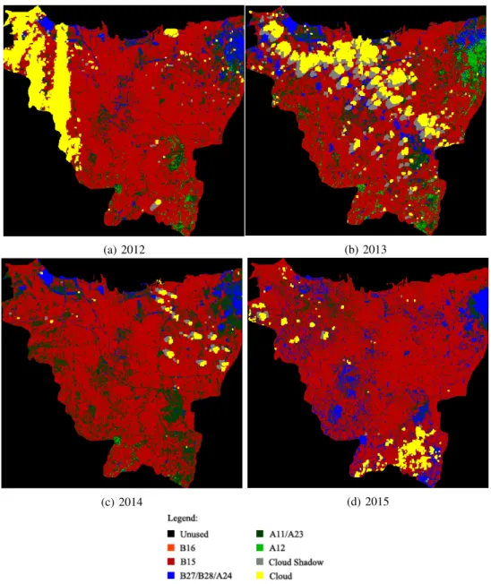
from 2012 to 2015. These generated estimated ground truth can be seen in fig 5. The pixels distribution among classes in the ground truth data is shown in fig. 4. From fig. 5, it can be seen that the classification model is often confused class A11/A23 and A12 with class B27/B28/A24. This fact may be caused by the similarity between cropland when flooded and waters. Class A11/A23 and A12 are also often confused with one another. The fact that they both represent vegetation area may be the reason of this confusion. The numbers of pixels that can be analyzed also depends on the weather characteristics of the image. For example, in fig. 5a and 5b, there are notable amount of pixels that cannot be analyzed because of cloud coverage. Due to this fact, B15 class area seems to grow significantly from 2013 to 2014. In fact, the reason is just because of the significant amount of B15 area covered by cloud in year 2013.
Fig. 4: Estimated ground truth class pixels distribution.
VI. CONCLUSION
This paper has demonstrated LULC dataset construction via classification. The estimated ground truth of dataset for years 2012 to 2015 has been successfully generated in this research. The estimated ground truth is generated using NN with single hidden layer of 30 nodes. This algorithm is choosen because it has the best performance among other tested algorithm, with the test accuracy of 75.41%.
In the future, it would be necessary to find a solution to overcome the problem of imbalanced class size proportion. It can be done, for example, by reformulating the major class so that the data contained in each classes are about the same to each other. It would also be important to try exploiting other classification method such as object-based classification for the future works. Another interesting method that can be exploited is the use of deep learning algorithm. Though it is
not frequent to be used in remote sensing, it is promising for deep learning algorithm to show a better result than what this research has already obtain. This is due to the fact that it has shown an amazing result in image processing area, which is similar to remote sensing area that also exploit visual data.
REFERENCES
[1] Y. Liu, G. Cao, Q. Sun, and M. Siegel, “Hyperspectral classification via deep networks and superpixel segmentation,”International Journal of Remote Sensing, vol. 36, no. 13, pp. 3459–3482, 2015. [Online]. Available: http://dx.doi.org/10.1080/01431161.2015.1055607
[2] V. Mnih and G. E. Hinton, “Learning to detect roads in high-resolution aerial images,” inComputer Vision–ECCV 2010. Springer, 2010, pp. 210–223.
[3] ——, “Learning to label aerial images from noisy data,” inProceedings of the 29th International Conference on Machine Learning (ICML-12), 2012, pp. 567–574.
[4] M. W. A. Halmy, P. E. Gessler, J. A. Hicke, and B. B. Salem, “Land use/land cover change detection and prediction in the north-western coastal desert of egypt using markov-ca,” Applied Geography, vol. 63, pp. 101 – 112, 2015. [Online]. Available: http://www.sciencedirect.com/science/article/pii/S0143622815001599 [5] H. Han, C. Yang, and J. Song, “Scenario simulation and the prediction of
land use and land cover change in beijing, china,”Sustainability, vol. 7, no. 4, pp. 4260–4279, 2015.
[6] A. Mondal, D. Khare, S. Kundu, and P. Mishra, “Detection of land use change and future prediction with markov chain model in a part of narmada river basin, madhya pradesh,” inLandscape Ecology and Water Management, ser. Advances in Geographical and Environmental Sciences, M. Singh, R. Singh, and M. Hassan, Eds. Springer Japan, 2014, pp. 3–14. [Online]. Available: http://dx.doi.org/10.1007/978-4-431-54871-3 1
[7] D. Mitsova, W. Shuster, and X. Wang, “A cellular automata model of land cover change to integrate urban growth with open space conservation,” Landscape and Urban Planning, vol. 99, no. 2, pp. 141 – 153, 2011. [Online]. Available: http://www.sciencedirect.com/science/article/pii/S0169204610002665 [8] J. J. Arsanjani, M. Helbich, W. Kainz, and A. D. Boloorani,
“Integration of logistic regression, markov chain and cellular automata models to simulate urban expansion,” International Journal of Applied Earth Observation and Geoinformation, vol. 21, pp. 265 – 275, 2013. [Online]. Available: http://www.sciencedirect.com/science/article/pii/S0303243411002091 [9] J. Han, Y. Hayashi, X. Cao, and H. Imura, “Application of an integrated
system dynamics and cellular automata model for urban growth assessment: A case study of shanghai, china,”Landscape and Urban Planning, vol. 91, no. 3, pp. 133 – 141, 2009. [Online]. Available: http://www.sciencedirect.com/science/article/pii/S0169204608002351 [10] J. O. Sexton, X.-P. Song, C. Huang, S. Channan, M. E.
Baker, and J. R. Townshend, “Urban growth of the washington, d.c.baltimore, {MD} metropolitan region from 1984 to 2010 by annual, landsat-based estimates of impervious cover,”Remote Sensing of Environment, vol. 129, pp. 42 – 53, 2013. [Online]. Available: http://www.sciencedirect.com/science/article/pii/S0034425712004130 [11] O. Dubovyk, G. Menz, C. Conrad, E. Kan, M. Machwitz, and A.
Khamz-ina, “Spatio-temporal analyses of cropland degradation in the irrigated lowlands of uzbekistan using remote-sensing and logistic regression modeling,”Environmental monitoring and assessment, vol. 185, no. 6, pp. 4775–4790, 2013.
(a) 2012 (b) 2013
(c) 2014 (d) 2015
Fig. 5: Illustration of ground truth data for year: (5a) 2012, (5b) 2013, (5c) 2014, and (5d) 2015
[12] D. d. C. Victoria, A. R. d. Paz, A. C. Coutinho, J. Kastens, and J. C. Brown, “Cropland area estimates using modis ndvi time series in the state of mato grosso, brazil,”Pesquisa Agropecu´aria Brasileira, vol. 47, no. 9, pp. 1270–1278, 2012.
[13] Z. Wu, P. S. Thenkabail, and J. P. Verdin, “Automated cropland classifi-cation algorithm (acca) for california using multi-sensor remote sensing,” Photogrammetric Engineering & Remote Sensing, vol. 80, no. 1, pp. 81– 90, 2014.
[14] (2015) The USGS website. [Online]. Available: http://www.usgs.gov/ [15] I. Mierswa, M. Wurst, R. Klinkenberg, M. Scholz, and T. Euler, “Yale:
Rapid prototyping for complex data mining tasks,” inProceedings of the 12th ACM SIGKDD international conference on Knowledge discovery and data mining. ACM, 2006, pp. 935–940.
[16] S. Shalev-Shwartz and S. Ben-David,Understanding Machine Learning: From Theory to Algorithms. Cambridge University Press, 2014. [17] V. Kotu and B. Deshpande, Predictive Analytics and Data Mining:
Concepts and Practice with RapidMiner. Morgan Kaufmann, 2014. [18] D. W. Hosmer Jr, S. Lemeshow, and R. X. Sturdivant,Applied logistic
regression. John Wiley & Sons, 2013, vol. 398.
[19] C. Cortes and V. Vapnik, “Support-vector networks,”Machine learning, vol. 20, no. 3, pp. 273–297, 1995.
[20] A. P. Engelbrecht,Computational intelligence: an introduction. John Wiley & Sons, 2007.
[21] S. Macchi and D. C. Council, “Development of a Methodology for Land Cover Classification in Dar es Salaam using Landsat Imagery,” 2014. [22] Z. Zhu, S. Wang, and C. E. Woodcock, “Improvement and expansion
of the fmask algorithm: cloud, cloud shadow, and snow detection for landsats 47, 8, and sentinel 2 images,” Remote Sensing of Environment, vol. 159, pp. 269 – 277, 2015. [Online]. Available: http://www.sciencedirect.com/science/article/pii/S0034425714005069 [23] Z. Zhu and C. E. Woodcock, “Object-based cloud and cloud
shadow detection in landsat imagery,” Remote Sensing of Environment, vol. 118, pp. 83 – 94, 2012. [Online]. Available: http://www.sciencedirect.com/science/article/pii/S0034425711003853 [24] (2015) Badan Informasi Geospasial (BIG), Indonesian Geospasial
Portal. [Online]. Available: http://portal.ina-sdi.or.id/
[25] BSN - National Standarization Agency of Indonesia, “Klasifikasi penutup lahan,” vol. SNI 7645, p. 28, 2010.
[26] J. Cohen et al., “A coefficient of agreement for nominal scales,” Educational and psychological measurement, vol. 20, no. 1, pp. 37–46, 1960.