Fast Parallel Machine Learning Algorithms for Large Datasets Using Graphic Processing Unit

(1)

Theses and Dissertations Graduate School

2011

Fast Parallel Machine Learning Algorithms for

Large Datasets Using Graphic Processing Unit

Qi Li

Virginia Commonwealth University

Follow this and additional works at:http://scholarscompass.vcu.edu/etd Part of theComputer Sciences Commons

This Dissertation is brought to you for free and open access by the Graduate School at VCU Scholars Compass. It has been accepted for inclusion in Theses and Dissertations by an authorized administrator of VCU Scholars Compass. For more information, please [email protected].

Downloaded from

(2)

(3)

DATASETS USING GRAPHIC PROCESSING UNIT

A Dissertation submitted in partial fulfillment of the requirements for the degree of Doctor of Philosophy at Virginia Commonwealth University.

by

QI LI

M.S., Virginia Commonwealth University, 2008

B.S., Beijing University of Posts and Telecommunications (P.R. China), 2007

Director: VOJISLAV KECMAN

ASSOCIATE PROFESSOR, DEPARTMENT OF COMPUTER SCIENCE

Virginia Commonwealth University Richmond, Virginia

(4)

ii

List of Tables

4.1 Performance comparison of symmetric Euclidean distance matrix

cal-culation. . . 32

4.2 Performance comparison of asymmetric Euclidean distance matrix

cal-culation. . . 33

4.3 Performance result of chunking method on real-world large datasets. . 37

4.4 K-NNS performance comparison on MNIST (60,000 data points, 576

features). . . 47

5.1 List of popular kernel functions. . . 55

7.1 The experimental datasets and their hyperparameters for the Gaussian

RBF kernel. . . 83

7.2 The accuracy performance comparison between GPUSVM and

LIB-SVM on small and medium datasets. . . 84

7.3 The speed performance comparison between GPUSVM and LIBSVM

on small datasets. . . 86

7.4 The speed performance comparison between GPUSVM and LIBSVM

on medium datasets. . . 87

7.5 The accuracy performance comparison between CPU and GPU on large

(8)

vi

7.6 The speed performance comparison between CPU and GPU on large

datasets. . . 92

7.7 The speed performance comparison among GPUSVM-S, GPUSVM-P

(9)

List of Figures

3.1 The architecture of a typical CUDA-capable GPU. . . 13

3.2 CUDA device memory model. . . 15

3.3 CUDA thread organization. . . 17

3.4 One level loop unroll in the kernel functions. . . 18

3.5 Non-coalesced reduction pattern and preferred coalesced reduction pat-tern. . . 20

3.6 Diﬀerent grid conﬁgurations for solving the vector summation problem among four vectors. . . 21

4.1 The complete distance matrix and its partial distance matrices. . . . 23

4.2 Impact of diﬀerent weights on classiﬁcation. . . 25

4.3 CUDA blocks mapping for generalized distance matrix calculation. . . 31

4.4 Mapping between data chunks to the related distance submatrices. . . 34

4.5 Map-Reduce pattern for large distance matrix calculation. . . 35

4.6 Speed performance comparison of sorting algorithms for ﬁxed k and various matrix dimension. . . 46

4.7 Speed performance comparison of sorting algorithms for various kand ﬁxed matrix dimension. . . 47

5.1 A graphic representation of linear SVM. . . 50

(10)

viii

5.3 One-Versus-All SVM classiﬁcation using Winner-Takes-All strategy. . 58

5.4 A graphic representation when both Lagrangian multipliers fulﬁll the

constraints. . . 60

5.5 The design structure for cache. . . 69

5.6 5-fold cross-validation steps for Gaussian kernels. . . 74

5.7 Binary linear SVM training on the same dataset with four diﬀerentC. 75

5.8 Same support vectors shared among the four tasks in Figure 5.7. . . . 75

6.1 GPUSVM: cross-validation interface. . . 78

6.2 GPUSVM: training interface. . . 79

6.3 GPUSVM: predicting interface. . . 79

7.1 The accuracy performance for diﬀerent values on medium datasets. 89

7.2 The number of support vectors for diﬀerentvalues on medium datasets. 90

7.3 The speed performance for diﬀerent values on medium datasets. . . 91

7.4 Training time comparison between GPUSVM and LIBSVM on large

datasets. . . 92

7.5 Predicting time comparison between GPUSVM and LIBSVM on large

datasets. . . 93

7.6 Independent task comparison on speed performance and number of

support vectors between GPUSVM and LIBSVM. . . 95

(11)

This dissertation deals with developing parallel processing algorithms for Graphic Pro-cessing Unit (GPU) in order to solve machine learning problems for large datasets. In particular, it contributes to the development of fast GPU based algorithms for calculating distance (i.e. similarity, aﬃnity, closeness) matrix. It also presents the algorithm and implementation of a fast parallel Support Vector Machine (SVM) us-ing GPU. These application tools are developed usus-ing Computus-ing Uniﬁed Device Architecture (CUDA), which is a popular software framework for General Purpose Computing using GPU (GPGPU).

Distance calculation is the core part of all machine learning algorithms because the closer the query is to some data samples (i.e. observations, records, entries), the

more likely the query belongs to the class of those samples. K-Nearest Neighbors

(k-NNs) search is a popular and powerful distance based tool for solving classiﬁcation

problem. It is the prerequisite for training local model based classifiers. Fast distance calculation can significantly improve the speed performance of these classifiers and GPUs can be very handy for their accelerations. Meanwhile, several GPU based

sorting algorithms are also included to sort the distance matrix and seek for the k

-nearest neighbors. The speed performances of the sorting algorithms vary depending upon the input sequences. The GPUKNN proposed in this dissertation utilizes the GPU based distance computation algorithm and automatically picks up the most suitable sorting algorithm according to the characteristics of the input datasets.

Every machine learning tool has its own pros and cons. The advantage of SVM is the high classiﬁcation accuracy. This makes SVM possibly one of the best classiﬁers. However, as in many other machine learning algorithms, SVM’s training phase slows

(12)

iii

down when the size of the input dataset increases. The GPU version of parallel SVM based on parallel Sequential Minimal Optimization (SMO) implemented in this dis-sertation is proposed to reduce the time cost in both training and predicting phases. This implementation of GPUSVM is original. It utilizes many parallel processing techniques to accelerate and minimize the computations of kernel evaluation, which are considered as the most time consuming operations in SVM. Although the many-core architecture of GPU performs the best in data level parallelism, multi-task (aka. task level parallelism) processing is also integrated into the application to improve the speed performance of tasks such as multiclass classification and cross-validation. Fur-thermore, the procedure of finding worst violators are distributed to multiple blocks on the CUDA model. This reduces the time cost for each iteration of SMO during the training phase. All of these violators are shared among different tasks in multiclass classification and cross-validation to reduce the duplicate kernel computations. The speed performance results have shown that the achieved speedup of both the training phase and predicting phase are ranging from one order of magnitude to three orders of magnitude times faster compared to the state of the art LIBSVM software on some well known benchmarking datasets.

(13)

Introduction

Machine learning is a discipline targeted on designing and developing algorithms which allow computers to learn based on empirical data and capture the characteris-tics of interest in order to make a prediction for a new data query. All the collected data can be considered as examples (training samples) which illustrate the relations among the observed variables. Many important patterns can be recognized after ap-plying the learning procedure. Supervised learning is one type of machine learning techniques inferring a function using supervised data, which does the classification or regression jobs. Classifiers are generated in the classification problems in which

both input feature vector xand the related output labely are known. They are used

for classifying new data queries and give discrete output. On the other hand, if the continuous output is required, a regression function will be created instead of a clas-sifier. This dissertation mainly focuses on classification problems. Currently, there are many well developed classification tools, e.g. Support Vector Machine, Neural

Network, Decision Tree, k-NNs search, etc. They all have certain advantages and

disadvantages in diﬀerent scenarios. However, one of the common drawback among them is the lack of scalability, which largely restricted their popularity and usage in processing large datasets. The fact is that it is an era of exploded information now,

(14)

2

and large scale datasets are found everywhere. For instance, a mid-size social network website can easily collect Tera-bytes of multimedia data such as users’ status change, newly uploaded photos, daily notes, conversations and so on. Most of these raw data are left unprocessed and archived due to the software limitations. However, these data can be very useful to help learn the users’ preferences, interests and patterns of their activities. The outcome is obvious. Better user experience always leads to more customers. Therefore, the newly improved many-core GPUs are involved to help re-duce the processing time for training large datasets. They are superbly fast in ﬂoating points operations and small in physical size. The hardware cost is also much less and so is the power consumption compared to CPUs which oﬀer the same level of pro-cessing capability. With the assists of GPUs, a proper equipped workstation can do just about the same job which could only be done on a small clustering system in the past. GPU’s popularity on solving data intensive applications is growing everyday. In this dissertation, GPUs are used for developing fast parallel SVM software.

This dissertation is mainly focusing on developing and implementing classifica-tion, a.k.a. pattern recogniclassifica-tion, algorithms for GPUs. The NVIDIA Tesla GPUs and CUDA software development kit are used as the main hardware and software components for the sake of software implementation. However, the proposed paral-lel processing algorithms, methodologies and optimization strategies are all original and general, which can be extended and adapted to other platforms or frameworks. They are all considered as the contributions of this dissertation. The final developed GUI enabled SVM tool which has been configured and installed in the department’s ACE-Tesla computer is also part of the contribution of this dissertation.

The original research objective includes the classic linear and non-linear SVM design as well as the local model based classiﬁers such as Local Linear SVM [1] and Adaptive Local Hyperplane [2]. The SVM part has been successfully ﬁnished in this

(15)

dissertation work. The crucial problem of the local model based classifiers, which is the distance computation, has also been addressed in the dissertation. In Chapter 2, some existing work done on both sequential and parallel SVM implementation are briefly reviewed. Major contributions of this dissertation are also listed in this chapter. Chapter 3 discusses the detail information about GPU and NVIDIA’s CUDA technology. CUDA programming model and optimization strategies are presented and explained to help understand the proposed implementations in the later chapters. Similarity search and distance computation is discussed in Chapter 4, which is the fundamental of building local model based classifiers. The speed performance of the proposed GPUKNN algorithm is also given. Chapter 5 reviews various decomposition approaches such as Platt’s SMO, Keerthi et al.’s improved SMO and Cao et al.’s parallel SMO in solving Quadratic Programming (QP) problem, which is the core of SVM solver. This chapter also introduces the proposed GPUSVM algorithm. Chapter 6 describes the hierarchy design architecture of the GPUSVM package. Chapter 7 presents the simulations and comparisons between the state of the art LIBSVM software and the GPUSVM software. The comparisons are done for both accuracy and speed performances on several benchmarking datasets of various sizes. The results have shown the impressive speed performance of the novel GPUSVM over LIBSVM while achieving very close accuracies. Chapter 8 gives the conclusions and points out some possible future work as the continuation of this dissertation.

(16)

Chapter 2 Background, Related Work and

Contributions

This chapter first briefly reviews the historical development of sequential SVM al-gorithms and parallel SVM algorithm. Parallel SVM algorithm used to be not very popular a decade ago compared to its sequential counterpart. There is much less re-search done on parallel SVM due to the lack of the availability for parallel hardware. However, it becomes more and more popular recently not only because sequential SVM suffers from a very slow training phase on large datasets, but also due to the huge improvement and the availability of the cheap and easy to program parallel

hardware. K-NNs search is another classic classiﬁcation tool, which recently has also

been used for building local model based classifiers. These classifiers have good ac-curacy and they can be trained efficiently in parallel. Some of these classifiers are

reviewed in this chapter. The core of k-NNs search is distance calculation which

has been addressed in this dissertation using powerful GPUs. Then several exist-ing mature parallel processexist-ing framework are discussed and compared to show their advantages and disadvantages. They are good options for creating parallel machine learning tools. At the end, the contributions of this dissertation are given.

(17)

2.1 The History of Sequential SVM

Support Vector Machine [3, 4] is a learning algorithm which has become popular due to its high accuracy performance. It solves both the classification and regression problems. Nevertheless, the training phase of an SVM could be a computationally expensive task especially for large datasets, because the core of the training is solving a QP problem. Solving large QP problem with numeric method can be very compli-cated, time consuming and memory inefficient. More details of solving QP problem are explained in Chapter 5. There are countless efforts and research which have been put on how to reduce the training time of SVM. After Vapnik invented SVM, he proposed a method known as “chunking” to break down the large QP problem into a series of smaller QP problems. This method seriously reduces the size of the matrix but it still cannot solve large problem due to the computer memory limitations at that time. Osuna et al. presented a decomposition approach using iterative meth-ods in [5]. Joachims introduced practical techniques such as shrinking and kernel caching in [6], which are common implementation in many modern SVM software. He also published his own SVM software called SVMLight [6] using these techniques. Platt invented SMO [7] to solve the standard QP problem by iteratively solving a QP problem with only two unknowns using analytic methods. This method requires very small amount of computer memory. Therefore it addresses the memory limitation issue brought by large training datasets. Kecman et al. [4] proposed the Iterative Single Data Algorithm (ISDA) which uses a single sample during every iteration of the optimization, which performs a coordinate descent search for a minimum of the cost function. ISDA has shown to have all the good properties of SMO algorithm while being slightly faster. Later on, Keerthi et al. developed an improved SMO in [8] which resolves the slow convergence issue in Platt’s method. More recently, Fan et al. introduced a series of working set selection [9], which further improves the speed

(18)

6

of convergence. These methods have been implemented and integrated in the state of the art LIBSVM software [10]. These major work summarize the background details of how to implement a fast classic SVM in sequential programming.

2.2 The Development of Parallel SVM

Compared to the sequential SVM, there is not much of research done on parallel SVM. However, the development of fast parallel SVM is still a very hot research topic. Some earlier works using parallel techniques in SVM can be found in [11], [12], [13] and [14]. Cao et al. presented a very practical Parallel Sequential Minimal Optimization (PSMO) [15] implemented with Message Passing Interface on a clustering system. The performance gain of training SVM using clusters shows the beauty of parallel processing. This method is also the foundation of the proposed GPUSVM here. Graf et al. introduced the Cascade SVM [16] which decomposes the training dataset to multiple chunks and trains them separately. Then the support vectors from different individual classifiers are combined and fed back to the system again. They proved that the global optimal solution can be achieved by using this method. This method uses task level parallelism compared to the data level parallelism in Cao et al.’s method. Cascade SVM offers a new way to handle ultra-large datasets training. Catanzaro et al. proposed a method to train a binary SVM classifier using GPU in [17]. Significant speed improvements were reported compared to the LIBSVM software. The latest GPU version of SVM was from Herrero-Lopez et al. [18]. They enabled the possibility to solve multiclass classification problems using GPU.

(19)

2.3 K

-Nearest Neighbors Search and Local Model

Based Classiﬁers

Although classic SVM shows its elegance in many aspects, researchers also put lots of efforts on other different variants of SVM. Some of them such as Iterative Single Data Algorithm mentioned earlier uses a single sample in solving QP problem. Others use approximate models such as Proximal SVM [19, 20]. Kecman et al. explore the possibility of combining local linear SVMs to approximate the global optimal solution in [1]. Similar work is also shown in [21, 22]. This local model idea starts an innovative trend with combination of various other classifiers. The Adaptive Local Hyperplane [2] is one of the best. Yang and Kecman’s results have shown that ALH beats most of other classifiers on classification accuracy for several popular datasets.

However, ﬁnding the optimal local model requires performing k-NNs search on the

training dataset. This can be very time consuming since the training stage must test

through a series of diﬀerent kvalues. One of the typical way of ﬁndingk-NNs is using

Tree structure [23]. However, this type of method has limited speed performance in the cases when training datasets have large feature space. Besides, doing repeated

individual k-NNs search is not very practical for training local model based classiﬁers

in terms of speed performance. The better approach would be computing the distance matrix of the training dataset in advance and then sort it with indexes by either rows

or columns. Thus k-NNs can be easily located in the index matrix with whatever

given k value without performing the search operation. The disadvantage of this

method is the high cost of the distance matrix computation. This disadvantage can be oﬀset by utilizing the computational power of GPUs. The earliest implementation of GPU based Euclidean distance calculation is introduced by Chang et al. in [24], but their proposed implementation is too simple to be useful in application design.

(20)

8

A more practical implementation can be found in [25]. The complete GPU KNN algorithm was ﬁrst implemented by Garcia et al. [26]. However, they use a modiﬁed insertion sort which only sorts a portion of the distance matrix. Thus it involves

duplicated distances computation when a series of k values are tested. Furthermore,

there are neither options for using other metrics nor for an inclusion of the weights in the distance computation. Weighted Euclidean distance computation is a necessary part of ALH algorithm. Our research is an extension of [25, 27] which includes the weighted Euclidean distance, cosine similarity and Manhattan distance calculation using GPUs. It will be integrated into the Local Linear SVM and ALH to improve their speed performance during the training phase in the future.

2.4 Parallel Computing Framework

There are many existing parallel programming tools and models proposed for differ-ent architecture of computer systems in the past decade. Message Passing Interface (MPI) [28] and OpenMP [29] are two of the most widely used parallel models which are designed for main stream computing systems. MPI is a model in which computing nodes do not share memory with each other. It is commonly used in a distributed environment such as a clustering system. All data sharing and exchange must be done through explicit message communications. A typical setup of MPI model in-cludes a master node and a group of slave nodes. The master node scatters the data to the slave nodes and gathers the results back after the computations have finished on the slave nodes. Most of the synchronizations are done on the master node. Per-formance of MPI system is highly related to the speed of intra-network connection due to the large amount of data exchange. Thus many MPI based algorithms are optimized to minimize these data exchange. The lack of the shared memory access across multiple computing nodes requires a significant amount of work on the

(21)

appli-cation design. OpenMP supports shared memory, which is more commonly used in the standard workstation systems and multi-core personal computers. Shared mem-ory system usually has a smaller scale compared to the distributed system. The scalability of OpenMP are restricted compared to MPI. Furthermore, the require-ment of precise threads managerequire-ment will not allow the OpenMP to generates many threads due to the cost of threads overhead, threads context switching and threads synchronization. Besides, if the amount of threads exceeds the number of computing cores, time-division multiplexing is used by computing cores to switch between phys-ical threads. Therefore it is less likely to improve the performance by creating more threads, which just involves extra computations. The advantage of OpenMP is the boost on the performance of existing applications by using multi-core system with minimal amount of modiﬁcations on the original algorithms if they are applicable. For example, algorithms running data independent tasks in a large loop structures can be easily accelerated with OpenMP.

GPU’s programming model is kind of a mixture of both message passing and shared memory with some of its own unique features. First of all, there is no shared memory access between GPUs and CPUs. All the data must be transferred from the main memory to the device memory for processing, which behaves the same

as MPI model does. Secondly, there are shared memory which can be accessed

by all threads within a block but threads from diﬀerent blocks inside of the GPU. This shows certain similarity feature to shared memory model. Furthermore, GPU threads are lightweight and eﬃcient. They are much simpler in structure compared to CPU threads with less overhead, which makes it possible to generate huge amount of threads for massive parallel processing. More details about GPU programming model will be introduced in Section 3.2. More recently, several major industry players including Apple, Intel, AMD/ATI and NVIDIA have jointly developed a

(22)

standard-10

ized programming model called Open Computing Language (OpenCL) [30]. OpenCL shares many common aspects from CUDA but it is still not very mature which makes it less popular on NVIDIA GPUs. Therefore CUDA is used for implementing the proposed algorithm in order to achieve the maximum speed gain by using the latest hardware from NVIDIA.

2.5 Contributions of This Dissertation

Although there is plenty of research done using GPU to improve speed performance of complex algorithms, many applications are still theory oriented and lack practical usage. This dissertation not only introduces the parallel SVM algorithm and distance calculation algorithms designed for GPU programming, but it also implements them using CUDA framework and makes them practical for processing real-world datasets. As it has been mentioned in the previous section, the author develops the algorithms in a way that they can be ported to other platform such as OpenCL. The GPUKNN search algorithm introduced in this dissertation, which is the fundamental for the use of local model based classiﬁers, combines the fast distance calculation and sorting

using GPU. By largely reducing the time cost ofk-NNs search, the speed performance

of LLSVM and ALH is expected to be improved heavily. Furthermore, not only does this practical application oﬀer the choice for diﬀerent distance metrics, but it is also smart to pick up the proper sorting algorithm for the best performance depending upon the characteristics of input datasets.

The CUDA implementation of parallel SVM developed in this dissertation has achieved great performance using Fermi series Tesla GPUs, which are the second generation hardware platform for CUDA. The software utilizes the parallelism in both data level and task level to maximize the performance of one single GPU card or several GPU cards operating simultaneously. It also leverages the computation

(23)

load between CPU and GPU. This helps improving the efficiency of the GPUSVM algorithm. The current implementation of the GPUSVM outperforms the state of the art LIBSVM tool in speed performance for both training phase and predicting phase. It also has as good accuracy performance as LIBSVM. Besides, the software is compatible with previous generation of GPUs and it is practical in solving real-world problems. It supports multi-GPU system to enable even further speed improvement on cross-validation training, which is a slow procedure on classic sequential machines. The software is developed using a three-layer structure. The bottom layer written in CUDA has an SVM solver and a predictor for SVM training and predicting functions. The middle layer written in Python offers command line interface to call the solver and predictor. It also contains utility functions of scaling the data files, shuffling the input datasets, running cross-validations and some other tasks related to SVM. The upper layer written in JAVA offers a user friendly graphic user interface for easy operation.

(24)

Chapter 3 Graphic Processing Units

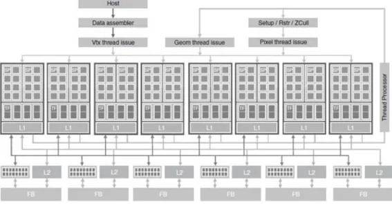
GPUs are micro processors commonly seen on video cards. The main function of GPU is offloading and accelerating the graphic rendering jobs from the CPU. Rendering is a process of generating an image from a model by a set of computer programs and it usually involves floating point intensive computations based on various mathemat-ical equations. Thus, before 2006, most of these GPUs were designed in a way that computing resources were partitioned into vertexes and pixel shaders. Even though the hardware of GPUs have matured for intensive floating point computations, there is no other way but using OpenGL or DirectX to access the features in GPUs. Smart programmers disguised their general computations to graphic problems in order to utilize the hardware capability of GPU. They were the first who started to use GPUs to solve general purpose computing problems. In order to overcome this inflexibility, NVIDIA introduced the GeForce 8800 GTX in 2006, which maps the separated pro-grammable graphics stages to an array of unified processors. Figure 3.1 shows the shader pipeline of GeForce 8800 GTX GPU. It is organized into an array of highly threaded streaming processors (SMs). In Figure 3.1, two SMs form a building block; however, the number of SMs in a building block can vary between different genera-tions of CUDA GPUs. Each SM in Figure 3.1 has a number of streaming processors

(25)

(SPs) that share control logic and instruction cache. Each GPU currently comes with up to 6GB (e.g. Tesla C2070) GDDR DRAM, referred to as global memory. These global memory are essentially the frame buﬀer memory that is used for graphics. For graphics applications, they hold video images and texture information for render-ing, but for computing purpose they function as high bandwidth oﬀ-chip memory. All later GPU products from NVIDIA follow this design philosophy thus they are capable of general purpose computing and referred to as CUDA capable devices.

Figure 3.1: The architecture of a typical CUDA-capable GPU.

The latest Tesla GPU has the shader processors (cores) fully programmable with large instruction memory, instruction cache and instruction sequencing control logic. In order to reduce the total hardware cost, several shader processors will share the same instruction cache and instruction sequencing control logic. The Tesla architec-ture introduced a more generic parallel programming model with a hierarchy of par-allel threads, barrier synchronization and atomic operations to dispatch and manage highly parallel computing work. Combined with C/C++ compiler, libraries, runtime

(26)

14

software and other useful components, CUDA Software Development Kit is oﬀered to developers who do not posses the programming knowledge of graphic applications. With a minimal learning curve of some extended C/C++ syntax and some basic parallel computing techniques, developers can start migrating existing projects using CUDA with NVIDIA GPUs. Introductions of CUDA programming model and its related optimization strategies are given in the following sections.

3.1 Computing Uniﬁed Device Architecture

(CUDA)

CUDA is a software platform developed by NVIDIA to support their general purpose computing GPUs for easy programming and porting existing applications to GPUs. It primarily uses C/C++ syntax and a few new keywords as an extension, which oﬀers a very low learning curve for an application designer. The latest CUDA version has been supported by various third parties. Many toolboxes and plug-ins can be found to help increase the productivity. CUDA memory model and thread organization is introduced in this part.

3.2 CUDA Programming Model

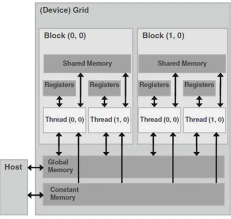
Figure 3.2 shows the memory model of the CUDA device. The device codes can read-/write per-thread registers; readread-/write per-block shared memory; readread-/write per-grid global memory; read only per-grid constant memory. The host codes can transfer data to/from per-grid global and constant memory. Constant memory oﬀers faster memory access to CUDA threads compared to global memory. The threads are or-ganized in a hierarchical structure. The top level is a grid which contains blocks of

(27)

Figure 3.2: CUDA device memory model.

threads. Each grid can contain at most 65535 blocks in either x- or y-dimension or

both in total. Each block can contain at most 1024 (Fermi series) or 512 threads

in either x- or y- dimension, or maximally 64 in z-dimension. The total number of

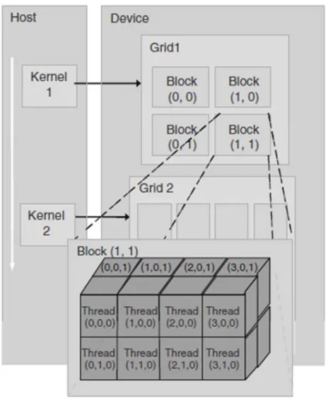
threads in all three dimensions must be less than or equal to 1024 or 512 depending on the hardware speciﬁcation. The organization of threads is shown in Figure 3.3. The host (CPU) launches the kernel function on the device (GPU) in the form of grid structure. Once the computation is done, the device becomes available again then the host can launch another kernel function. If multiple devices are available at the same time, every kernel function can be managed through one CPU thread. It is fairly easy to launch a grid structure containing thousands of threads. The optimum number of

(28)

16

thread and block configuration varies among different applications. To achieve bet-ter performance, there should be at least thousands or tens of thousands of threads within one grid. It would not make much sense to use too few threads to extract maximal performance from hardware. However, too many threads whose number exceeds the number of data would also increase the thread overhead and bring down the efficiency. The multiprocessor creates, manages, schedules, and executes threads in groups of 32 parallel threads called warps. Thus a multiple of 32 could be a good candidate value for the optimal number of threads per block. Threads within the same block have limited shared memory and they are able to communicate with each other by using these shared memory. All threads have their own registers and access to the global memory as well as the constant memory. The size of the global memory can be as large as up 6GB (depending on the GPU hardware). Similar to Message Passing Interface (MPI), there is no shared memory between host and device thus the data must be transferred from the host memory to device memory in the first place. The result must also be transferred back for future processing or storage.

3.3 CUDA Optimization Strategy

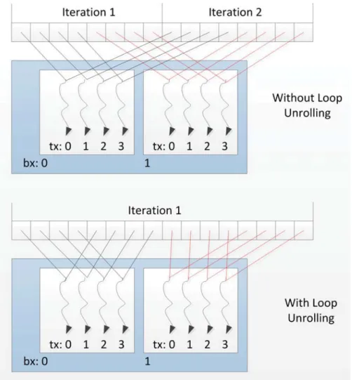
Optimizations generally are targeted on improving certain algorithms with maximum utilization of hardware. Several techniques which have been used in the proposed algorithms are given here. The ﬁrst one is loop unrolling which is shown in Figure 3.4. Loop unrolling has been used in sequential programming for a long time. Most modern compilers automatically unroll the loop in certain degrees to achieve better performance. In the simple example below, the loop structure is executed only once in the unrolled version instead of twice in the normal version. The advantage is that each thread can now process two data elements without using an extra loop. It is true in most situations that not enough threads can be created to match the total

(29)

Figure 3.3: CUDA thread organization.

number of data. Thus, each thread may process more than one data element, which requires the usage of loop structure. Think about how to write a code to do vector summation in sequential way. It can be done like this:

int idx = 0;

while( idx < n ) {

sum [ idx ] = a [ idx ] + b [ idx ];

(30)

18

Figure 3.4: One level loop unroll in the kernel functions.

}

Similarly, writing a CUDA kernel function to do the same job looks like the following:

int idx = b l o c k I d x . x * b l o c k D i m . x + t h r e a d I d x . x ;

int s h i f t = g r i d D i m . x * b l o c k D i m . x ;

while( idx < n ) {

sum [ idx ] = a [ idx ] + b [ idx ];

idx += shift ;

(31)

To reduce the overhead of loop, common practice suggests doing one level of loop unrolling as shown below.

int idx = b l o c k I d x . x * ( b l o c k D i m . x * 2) + t h r e a d I d x . x ;

int s h i f t = g r i d D i m . x * b l o c k D i m . x * 2;

while( idx < n ) {

sum [ idx ] = a [ idx ] + b [ idx ];

if( idx + b l o c k D i m . x < n ) {

sum [ idx + b l o c k D i m . x ] = a [ idx + b l o c k D i m . x ] + b [ idx +

b l o c k D i m . x ];

}

idx += shift ;

}

CUDA compiler does not support automatic loop unrolling like sequential program-ming compilers due to the complexity of condition checking mechanism. Thus it is the developers’ job to write loop unrolling statements in the source code.

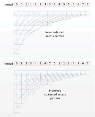
Another commonly used technique is reduction. Because threads from different blocks cannot communicate with each other, the results returned from each block compose a vector. In most applications, since the results are distributed to many blocks for parallel processing, they require the summation of the distributed results and this is so called reduction. Figure 3.5 shows both inefficient reduction pattern and preferred reduction pattern. It is important to let the threads access the global memory in a coalesced manner to achieve the best performance. The correct imple-mentation of reduction technique is much more complex than what is shown in the figure. Threads must be synchronized at every stage and reductions stop at the block level since there are no threads communication among blocks. Thus, to compute the final result the complete reduction will require multiple launches of kernel functions with reduced grid size until the total number of blocks in the grid becomes one. Re-duction can be utilized to implement MAX, MIN, SUM and some other functions

(32)

20

which are basic but very useful.

Figure 3.5: Non-coalesced reduction pattern and preferred coalesced reduction pat-tern.

The third commonly used technique is the utilization of shared memory. GPUs are fast on floating points operations but not on memory accessing operations. If a program requires frequently access to memories, it might not be able to achieve better performance by using GPUs. Although GPU can have global memory as large as 6GB, the amount of shared memory is very limited. Assuming a problem which computes summations of any two vectors among four different vectors, there are six different combinations as a group of two vectors. Thus creating six rows of blocks to compute the results is most intuitive idea as our first response. However, this

(33)

configuration is shown as Grid 0 in Figure 3.6. Each vector must be read three times from the global memory. Instead, Grid 1 configuration reduces the number of reads for the same vectors to two, but every row block must compute two results. In order to let the threads share data between two vector summations, shared memory must be involved to store the data read from the global memory. In the configuration of

Grid 2, vectorAis read only once but all other vectors are read twice. This does very

small improvement compared to Grid 1 in terms of memory accessing operations but it requires much more shared memory, which might be not satisfied in some scenarios. Thus, how to design the grid configuration and maximize the usage of limited shared memory is an important concern for producing efficient codes. One good example is the matrix multiplication which can be found in CUDA SDK sample codes. Our fast distance computation routine in the next Chapter carries similar idea behind the scene.

Figure 3.6: Diﬀerent grid conﬁgurations for solving the vector summation problem among four vectors.

(34)

Chapter 4 Similarity Search on Large

Datasets

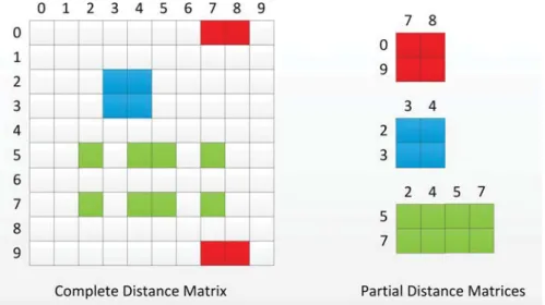
Measuring similarity (i.e. distance, aﬃnity, closeness) between diﬀerent samples is the fundamental approach in pattern recognition. This approach is based on the belief that the closeness in a feature space means similarity between two samples. Similarity search is based on the comparisons among distances. Euclidean, cosine and Manhat-tan disManhat-tances are common similarity metrics which are used in many machine learning algorithms. The idea behind the similarity search is that a smaller distance between two data points may indicate a stronger or closer relationship between them. General distance matrix for a dataset is a symmetric square matrix containing distances from each data point to all other data points including itself. When the total number of samples grows large, it is usually not feasible to compute or store the complete distance matrix in the system memory. For example, a dataset containing 100,000 samples could cost approximately 40GB space in single precision format and twice of that in double precision. Obviously, half of them can be reduced due to the symmetric property, however it is still not practical in real-world application design. Therefore most of distance computations are done in real time or precalculated in advance. A

(35)

fragment of the complete distance matrix is referred to as a partial distance matrix shown in Figure 4.1. It contains distances between one set of data points to another set of data points, which could have diﬀerent number of samples. Partial distance matrix can be asymmetric and rectangular. It is used for reproducing the original complete distance matrix.

Figure 4.1: The complete distance matrix and its partial distance matrices.

This chapter addresses the issue of how to utilize the power of GPU to accelerate the time consuming distance matrix computation. The deﬁnitions of three major distance kernels are given at the beginning and then the classic algorithms as well as the parallel algorithm using CUDA for distance calculation are introduced. Data partitioning and distributed computing techniques for large distance matrix are also presented. And then a few parallel sorting algorithms are given to build the complete GPU based GPUKNN software. This tool has a good speed performance in solving

k-NNs search problem compared to the classic sequential algorithm. The results of

the speed performance on calculating distance matrix, sorting and the GPUKNN are given at the end of the chapter.

(36)

24

4.1 Distance Deﬁnition

Deﬁne two matricesAandB. Acontainsn_Asamples and each sample hasmfeatures.

Each row represents one data sample from the dataset. B has nB samples and it is

organized in the same format asA. The distance matrixD_ABbetweenAandBis an

n_A by n_B matrix where each row represents the distances between one data sample

from A to all data samples from B. The distance value d_ij represents the distance

between data sample a_i and data sample b_j.

4.1.1 Weighted Euclidean Distance

Weighted Euclidean distance is a more generalized Euclidean distance, also known

as weighted L₂-norm distance, which oﬀers the option of specifying a weight for each

diﬀerent feature. It is deﬁned by

dij = m k=1 wk(aik−bjk)2. (4.1)

When all weights are equal to one, weighted Euclidean Distance becomes to the

stan-dard Euclidean Distance. If w_k = 0, the kth feature will be eliminated in distance

calculation. Weighted Euclidean distance becomes useful when the features have dif-ferent impacts on the classiﬁcation result. In Figure 4.2, the solid green line deﬁnes the best separation boundary. Both features must be used for computing this separa-tion line. However, the dashed yellow line can also separate the two classes without

any failure and it only uses feature 1. It is obvious that correct classiﬁcation cannot

be done using just feature 2. This indicates that using a bigger weight for feature

1 compared to feature 2 might yield better classiﬁcation result. If the weights are

proper chosen, weighted Euclidean distance performs better than standard Euclidean distance. Many advanced machine learning models such as ALH in [2] use weighted

(37)

Figure 4.2: Impact of diﬀerent weights on classiﬁcation.

Euclidean distance.

4.1.2 Cosine Similarity

Cosine similarity, a.k.a. cosine distance is deﬁned as

d_ij = a T i ·bj a_ib_j = m k=1 aikbjk m k=1 a2_ik m k=1 b2_jk . (4.2)

Cosine similarity is a useful measurement in documents comparison and text mining. Weighted cosine similarity is not widely used.

(38)

26

4.1.3 Weighted Manhattan Distance

Weighted Manhattan distance is another popular distance measurement similar to

weighted Euclidean distance. It is also referred as weighted L₁-norm distance, which

is deﬁned as d_ij = m k=1 w_k|a_ik−b_jk| (4.3)

4.2 Distance Calculation Algorithms

4.2.1 Classic Sequential Method

Algorithm 1 shows the standard procedure of calculating distances between two

datasets. This method involves a nested for loopstructure, which leads to a

polyno-mial time complexity ofO(n_An_Bm) a.k.a. cubic time. Considering the size of feature space is much smaller than the number of data samples, the time complexity is

re-duced to quadraticO(n2) in many cases. However, algorithms having quadratic time

complexity are still very slow and time consuming. A good property of Euclidean distance is that the computations for the distance matrix can be broken down to matrix level operations. In this way, the nested loop structure for pair-wise distance computation can be removed. This is shown in Algorithm 2.

The idea of this algorithm is computing the weighted Euclidean distance matrix using three partial distance matrices directly shown in Equation 4.4 instead of com-puting every pair of distance one by one using loops.

D_AB =P₁+P₂−2P₃. (4.4)

(39)

Algorithm 1 Classic sequential distance calculation using loops.

1: load A,B, w and allocate memory forD_AB

2: for i= 1 to n_A do 3: for j = 1 to n_B do 4: d_ij = computeEucDist(a_i,b_j, w) 5: or d_ij = computeCosDist(a_i,b_j) 6: or d_ij = computeManDist(a_i,b_j,w) 7: end for 8: end for 9: return D_AB 10: computeEucDist(a_i,b_j, w) 11: d= 0 12: for k = 1 to m do 13: d=d+w_k(a_ik−b_jk)2 14: end for 15: d=√d 16: return d 17: 18: computeCosDist(a_i,b_j) 19: p=p_a= p_b = 0 20: for k = 1 to m do 21: p=p+a_ikb_jk 22: p_a=p_a+a_ika_ik 23: p_b =p_b+b_jkb_jk 24: end for 25: d=p/(√p_a√p_b) 26: return d 27: 28: computeManDist(a_i,b_j,w) 29: d= 0 30: for k = 1 to m do 31: d=d+wk|aik−bjk| 32: end for 33: return d

(40)

28

Algorithm 2 Matrix operation based method for weighted Euclidean distance.

1: load A,B, w and allocate memory forD_AB

2: v₁ = (A·A)w 3: v₂ = (B·B)w 4: P₁= [v₁v₁ . . . v₁] 5: P₂= [v₂v₂ . . . v₂]T 6: W = [w w . . . w]T 7: P₃=A(B·W)T 8: D_AB =√P₁+P₂−2P₃ 9: return D_AB

partial distances matrices are P₁, P₂ andP₃ and they are expressed as

P₁ = ⎡ ⎢ ⎢ ⎢ ⎢ ⎢ ⎢ ⎢ ⎣ m k=1 w_ka2₁_k · · · m k=1 w_ka2₁_k .. . . .. ... m k=1 wka2nAk · · · m k=1 wka2nAk ⎤ ⎥ ⎥ ⎥ ⎥ ⎥ ⎥ ⎥ ⎦ = [v₁v₁ . . . v₁]. (4.5) P₂= ⎡ ⎢ ⎢ ⎢ ⎢ ⎢ ⎢ ⎢ ⎣ m k=1 w_kb2₁_k · · · m k=1 w_kb2_n_B_k .. . . .. ... m k=1 w_kb2₁_k · · · m k=1 w_kb2_n_B_k ⎤ ⎥ ⎥ ⎥ ⎥ ⎥ ⎥ ⎥ ⎦ = ⎡ ⎢ ⎢ ⎢ ⎢ ⎢ ⎢ ⎢ ⎣ v₂T vT 2 .. . vT 2 ⎤ ⎥ ⎥ ⎥ ⎥ ⎥ ⎥ ⎥ ⎦ . (4.6) P₃ = ⎡ ⎢ ⎢ ⎢ ⎢ ⎢ ⎢ ⎢ ⎣ m k=1 w_ka₁_kb₁_k · · · m k=1 w_ka₁_kb_n_B_k .. . . .. ... m k=1 w_ka_n_A_kb₁_k · · · m k=1 w_ka_n_A_kb_n_B_k ⎤ ⎥ ⎥ ⎥ ⎥ ⎥ ⎥ ⎥ ⎦ . (4.7)

MatricesP₁andP₂ shown in Equation 4.5, 4.6 are composed by vectorv₁ and vector

v₂. The weight vector w is shown in

(41)

Vector v₁ is acquired by v₁ = [ m k=1 wka21k, m k=1 wka22k, ..., m k=1 wka2nAk]T = (A·A)w (4.9)

and vectorv₂ is acquired by

v₂ = [ m k=1 w_kb2₁_k, m k=1 w_kb2₂_k, ..., m k=1 w_kb2_n_B_k]T = (B·B)w. (4.10)

The partial distance matrix P₃ is computed by

P₃ =A(B·W)T. (4.11)

When all weights are equal to 1, the weighted Euclidean distance becomes standard Euclidean distance and Equation 4.11 changes to

P₃ =ABT. (4.12)

The matrix multiplication in Equation 4.11 or 4.12 takes most of the computation time in Euclidean distance calculation. The naive implementation yields exact same quadratic time complexity. However, CUDA has its own fast Basic Linear Algebra Subroutines called CUBLAS [31]. The weighted Euclidean distance calculation can be accelerated by calling matrix-matrix multiplication routine from CUBLAS. This im-plementation turns out to have improved time complexity compared to the quadratic one. When it comes to the cosine similarity and weighted Manhattan distance, there is no way to transform the distance matrix computations to simple matrix

(42)

opera-30

tions thus routines from CUBLAS are useless. Although, the time complexity stays in quadratic, the time cost of distance computations can still be reduced by using parallel techniques. A general GPU based parallel distance computation algorithm is introduced in the following section. It can be used for all three metrics and it oﬀers as good speed performance as using CUBLAS for weighted Euclidean distance computations as well.

4.2.2 Parallel Method Using CUDA

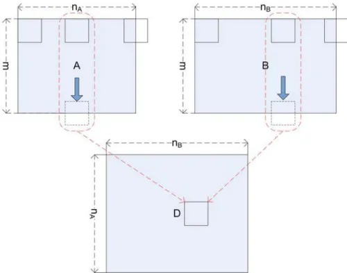
In order to map the distance calculation to the CUDA programming model, the GPU kernel function utilizes a 2-D grid and uses shared memory to reduce the duplicated memory fetching operations. The size of the block within the grid is set to 16 by 16. The following code is used for initialization.

# d e f i n e B L O C K _ D I M 16

dim3 d i m B l o c k ( BLOCK_DIM , BLOCK_DIM ,1) ;

dim3 dimGrid (( nA + BLOCK_DIM -1) / BLOCK_DIM ,

( nB + BLOCK_DIM -1) / BLOCK_DIM ,1) ;

In this way, the size of the grid will depend upon the input. It overcomes the imple-mentation issue in [24] and supports input datasets with any dimensionality and any number of data points. The pseudo code provided in [24] requires the input feature space as a multiple of 32 and the input number of data points as a multiple of 2, which are not practical in real-world applications. Figure 4.3 shows how the kernel function works. Most blocks compute 256 pairwise distances. Some blocks located on the bottom edge or the right edge of the grid may compute less than 256 pairwise distances. That means some threads allocated in these blocks are not involved for the computation. This cannot be avoid when the input datasets are irregular, which do not have the number of data points as a multiple of 16. The shared memory is used for storing the values of the features and the values of the weights. Feature values can

(43)

be reused in calculation of 16 pairwise distances and the weight values can be reused in calculation of all 256 pairwise distances in that block. This signiﬁcantly reduces the time cost of global memory access.

Figure 4.3: CUDA blocks mapping for generalized distance matrix calculation.

4.3 Performance Results of Distance Kernel

Function

The following results are published in [25] generated by a workstation equipped with the ﬁrst generation of Tesla cards. The workstation has an Intel Xeon E5462 2.8GHz quad-core CPU and 16GB RAM. There are three Tesla C1060 GPU devices connected to the system through PCI Express interface. Each of these cards has 4GB device memory. The CUDA 3.0 toolkit is used and the driver version is 195.36.15 for 64bit

(44)

32

Linux system. The operating system is Fedora Core 10 Linux. The benchmark of GPU algorithms includes two ways of data transferring time between host memory and device memory as well as the computational time on the GPU.

Table 4.1 shows the normal Euclidean distance matrix calculation comparison among naive C implementation, MKL based C implementation, Chang et al.’s CUDA implementation [24], and the proposed generalized CUDA implementation. It is easy to observe that using MKL and multi-thread support for CPU can boost the perfor-mance 5 to 6 times, thus comparison with the naive C implementation does not truly reﬂect the performance gain by using GPU. Our implementation is slightly slower in

these special cases (both nandm are multiple of 16) compared to Chang et al.’s

im-plementation because the kernel function has been modiﬁed to suit general datasets, which cannot be used by Chang et al.’s method. It takes two datasets as input, thus the same dataset is copied twice from the system memory to the device mem-ory in theses special cases. In general, the GPU implementation still has a speed-up of approximately 5 times compared to MKL which is in the reasonable range based on the performance comparison of matrix-matrix multiplication between MKL and CUBLAS shown in [32].

Table 4.1: Performance comparison of symmetric Euclidean distance matrix calcula-tion.

Input matrix Naive Eﬃcient Chang et al.’s Generalized

n C C (MKL) CUDA CUDA

4096 11.9 2.40 (4.96x) 0.36 (33.06x) 0.47 (25.32x)

8192 48.4 8.49 (5.70x) 1.42 (34.08x) 1.79 (27.04x)

12288 108.8 18.26 (5.96x) 3.16 (34.40x) 3.82 (28.48x)

Time unit is second and the size of feature space is 1024. Speed up is related to the

naive C implementation. Value n is number of data points.

(45)

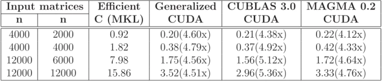
matrix between any two input datasets. Chang et al.’s method is not listed because of the unsuitability. CUBLAS 3.0 based implementation comes at the top and the proposed generalized CUDA implementation is very close to the GPU matrix oper-ation based method. Other distances matrices, e.g. Manhattan distance and cosine distance, cannot be eﬃciently transformed to matrix level operations. However, they still can be easily implemented by modifying the proposed method.

Table 4.2: Performance comparison of asymmetric Euclidean distance matrix calcu-lation.

Input matrices Eﬃcient Generalized CUBLAS 3.0 MAGMA 0.2

n n C (MKL) CUDA CUDA CUDA

4000 2000 0.92 0.20(4.60x) 0.21(4.38x) 0.22(4.12x)

4000 4000 1.82 0.38(4.79x) 0.37(4.92x) 0.42(4.33x)

12000 6000 7.98 1.75(4.56x) 1.56(5.12x) 1.72(4.64x)

12000 12000 15.86 3.52(4.51x) 2.96(5.36x) 3.33(4.76x)

Time unit is second and the size of feature space is 1000. Speed up is related to the

eﬃcient C implementation. Value n is number of data points.

4.4 Data Partitioning and Distributed

Computation

Considering scenarios with large datasets, all data points can neither be loaded into the system memory at one time, nor is there enough space for storing the complete distance matrix. It would be necessary to break down the complete distance matrix into many small distance matrices and calculate them individually in parallel. Figure 4.4 shows the approach of how to split the input datasets to chunks and calculate the generalized distance matrices between any two chunks. Each chunk is assigned

(46)

34

matrices. Due to the symmetric property of the complete distance matrix, there are

only k(k+ 1)/2 small distance matrices required to be calculated in a total of k2

ones. The rest of them can be acquired by simply doing transpose operation on the

calculated ones, e.g. D(1,2) is the transpose ofD(2,1). The performance gaing can

be roughly computed by

g= k−1

2k ·100%. (4.13)

For example, if the input dataset is split to 4 chunks, only 10 small distance matrices

Figure 4.4: Mapping between data chunks to the related distance submatrices.

out of 16 are required to be computed. This roughly saves 37.5% of total compu-tations. These small distance matrices can be calculated using the method, which is accelerated by GPU, introduced in the previous section. The amount of physical GPU devices determines how many grids can be launched simultaneously.

The Map-Reduce [33] pattern has been proposed to handle large data processing problems in a cluster environment. The merits of this programming pattern is adopted and modeled to do the large distance matrix calculation job. As shown in Figure 4.5,

(47)

Figure 4.5: Map-Reduce pattern for large distance matrix calculation.

the input reader first reads multiple chunks into the system memory. Then the mapper generates a list of key/value pairs, which correspond to these active chunks currently loaded in the system memory. For each key/value pair, both key and value store the indices of the chunks. The reducers iteratively load pairs of chunks with the same key and search for any available GPU device to launch the distance kernel function. There is a list which stores the IDs of the available GPUs. Any GPU device which is taken by a reducer will be removed from the list and appended back after it is released by that reducer. Each reducer only calculates the small distance matrices whose keys are smaller than or equal to their values. The final distance matrix is in the form of its upper triangular. After all small distance matrices with the same key are calculated by the reducer, the results are grouped together and passed to the output writer. The output writer concatenates the results from every reducer and writes them to a distributed file system if available. A drawback of this approach is that different reducers may have different workloads. This can be solved by fixing the number of small distance matrices calculation job to each reducer. For example, the first reducer calculates D(1,1) to D(1,5), the second calculates D(1,6) to D(1,10) and so on. However, the key value must still be kept the same in each reducer. In this way, only certain reducers might have less jobs. But in a general view, the distance calculations are distributed equally among reducers. When each reducer finishes its

(48)

36

job, it will notify the mapper to update the key/value pairs list and refresh the system memory by loading in new chunks and deleting used ones.

The complete model requires a GPU cluster environment and extra communi-cation support, e.g. MPI, from different nodes as well as a proper distributed file system. Our test is done on a workstation with three Tesla C1060 GPU devices. This is much simpler compared to the GPU cluster environment. Multi-threading is used for implementing different functions for input reader, maper, reducer and out-put writer. Since all reducers will be competing for the GPU device resources on the same computer, whether they have an equal amount of jobs does not matter anymore. Because all three cards will be used for distance matrices calculations all the time, an approximately performance increase of 3x is achieved compared to using one card to do the same job sequentially.

Table 4.3 shows the performance of ﬁnalized chunking method tested on the real-world datasets. File I/O time is excluded because both CPU and GPU implementa-tions share the same procedure. The time cost is counted for calculating submatrices only. The data transferring time for GPU is reduced because in certain cases some datasets can be reused. For example, if the same GPU is assigned to the job

calcu-lating D(1,1) andD(1,2), only chunk 2 needs to be loaded into the device memory

in the second distance matrix calculation. The speedup is close to 15 times when utilizing three GPU devices together on a dataset containing more than half million data points.

4.5 Parallel Sorting Using CUDA

Once the distance matrix is acquired, the parallel sorting algorithm can be applied

to locate the k-NNs. There are many classic sequential sorting algorithms available

(49)

Table 4.3: Performance result of chunking method on real-world large datasets.

Dataset n m Xeon c Tesla C1060 3 X Tesla C1060 4-core

Mnist 60,000 780 203.82s 4 48.43s 19.39s

(4.21x) (10.51x)

Covertype 581,012 54 54.21m 39 10.84m 3.62m

(5.00x) (14.98x)

Valuen is the number of data points. Valuemis the size of feature space. Valuec is

the number of chunks. Time unit is second and minute. Speed up is related to CPU implementation.

of them can be simply implemented using CUDA, some of these algorithm may not be able to fully utilize the power of GPU and they might be slower than the highly optimized versions using CPU. To achieve better performance, it is important to map the algorithm to the CUDA programming model and break down the problem to small pieces. Most classic sorting algorithms are covered in this section. However, only three major sorting algorithm are introduced to present the power of GPU. The first one is radix sort. It is part of the CUDA library. The detail of the implementation is given in [34]. An efficient merge sort is also introduced in the same paper. The second one is a modified insertion sort and the third one is a modified shell sort. They both have original implementations from the author and they are considerably fast for sorting arrays in certain scenarios. They compose part of the contribution

for this dissertation. Becausek-NNs search requires ﬁnding the indices of the nearest

neighbors, all sorting algorithms discussed here sort with indices.

4.5.1 Sequential Sort

Sorting algorithms such as quick sort and merge sort are classiﬁed as comparison sort. Comparison sort are based on comparison operations for ﬁnding the correct order of

(50)

38

the input sequence. The time complexity O(nlgn) is the best that comparison sorts

can achieve in the worst case. However, sorting algorithms which are not comparison based are not limited by this lower bound. For example, counting sort and bucket sort both can perform linear time sorting. These sorting algorithms usually have certain restraints for the input sequence which make them less popular for solving general sorting problems.

Merge Sort

Merge sort uses the typical divide and conquer technique. The merge operation assumes two input sequences being in either ascending or descending order. It merges the two input sequences into one piece with the correct order. The complete input sequence is broken down to multiple pairs of one element sequence. Then all of these sequences are merged starting from the bottom. The algorithm sample code is shown below.

t e m p l a t e < class T >

void merge ( T * array , int p , int r , int q ) {

T * n e w A r r a y = new T [ r - p + 1]; int idx = 0; int i = p ; int j = q ; while ( i <= q -1 || j <= r ) { if ( i == q ) { n e w A r r a y [ idx ++] = array [ j ++]; c o n t i n u e; } if ( j == r ) { n e w A r r a y [ idx ++] = array [ i ++]; c o n t i n u e; }

(51)

if ( array [ i ] < array [ j ]) { n e w A r r a y [ idx ++] = array [ i ++]; } else { n e w A r r a y [ idx ++] = array [ j ++]; } }

copy ( newArray , n e w A r r a y + ( r - p + 1) , array + p ) ;

d e l e t e [] n e w A r r a y ;

}

void m e r g e S o r t ( T * array , int p , int r ) {

if ( p < 0 || r < 0) { r e t u r n; } if ( r <= p ) { r e t u r n; } else if ( r - p == 1) { if ( array [ p ] > array [ r ]) {

swap ( array [ p ] , array [ r ]) ;

}

r e t u r n;

} else {

int q = p + (int) floor (( r - p + 1) / 2) ;

m e r g e S o r t ( array , p , q - 1) ;

m e r g e S o r t ( array , q , r ) ;

merge ( array , p , r , q ) ;

}

The advantage of merge sort is the stableO(nlgn) performance in both average case

and the worst case. However, the disadvantages are the recursive operation and the extra temporary memory space taken. Unluckily, both of them are very critical for

(52)

40

utilizing GPU power. Therefore, merge sort is not deep researched in this dissertation.

Quick Sort

Quick sort is probably the most popular and beautiful sort in many applications. It is the default sorting implementation in C++ standard template library. It is also the built-in sorting algorithm for many other programming language such as Java and Matlab. Unlike merge sort, quick sort is an in place sorting algorithm which requires only constant temporary memory space. The drawback of quick sort is that it has a quadratic time complexity in the worst case. However, the worst case rarely happens. The sample code of quick sort is given below.

int p a r t i t i o n ( T * array , int p , int r ) {

T pivot = array [ r ]; int i = p - 1; for (int j = p ; j < r ; ++ j ) { if ( array [ j ] <= pivot ) { ++ i ; if ( i != j )

swap ( array [ i ] , array [ j ]) ;

}

swap ( array [ i + 1] , array [ r ]) ;

r e t u r n i + 1;

}

void q u i c k S o r t ( T * arr , int p , int r ) {

if ( r == p )

r e t u r n;

if ( p < r ) {

Fast Parallel Machine Learning Algorithms for Large Datasets Using Graphic Processing Unit