Kernel Density Metric Learning

(1)

Washington University in St. Louis

Washington University Open Scholarship

All Computer Science and Engineering

Research

Computer Science and Engineering

Report Number: WUCSE-2013-28

2013

Kernel Density Metric Learning

Yujie He, Wenlin Chen, and Yixin Chen

This paper introduces a supervised metric learning algorithm, called kernel density metric

learning (KDML), which is easy to use and provides nonlinear, probability-based distance

measures. KDML constructs a direct nonlinear mapping from the original input space into a

feature space based on kernel density estimation. The nonlinear mapping in KDML embodies

established distance measures between probability density functions, and leads to correct

classification on datasets for which linear metric learning methods would fail. Existing metric

learning algorithms, such as large margin nearest neighbors (LMNN), can then be applied to the

KDML features to learn a Mahalanobis distance. We also... Read complete abstract on page 2.

Read complete abstract on page 2.

Follow this and additional works at:

https://openscholarship.wustl.edu/cse_research

Part of the

Computer Engineering Commons

, and the

Computer Sciences Commons

Recommended Citation

He, Yujie; Chen, Wenlin; and Chen, Yixin, "Kernel Density Metric Learning" Report Number: WUCSE-2013-28

(2013). All Computer Science and Engineering Research.

https://openscholarship.wustl.edu/cse_research/103

Department of Computer Science & Engineering - Washington University in St. Louis Campus Box 1045 - St. Louis, MO - 63130 - ph: (314) 935-6160.

(2)

This technical report is available at Washington University Open Scholarship: https://openscholarship.wustl.edu/ cse_research/103

Kernel Density Metric Learning

Yujie He, Wenlin Chen, and Yixin Chen

Complete Abstract:

This paper introduces a supervised metric learning algorithm, called kernel density metric learning

(KDML), which is easy to use and provides nonlinear, probability-based distance measures. KDML

constructs a direct nonlinear mapping from the original input space into a feature space based on kernel

density estimation. The nonlinear mapping in KDML embodies established distance measures between

probability density functions, and leads to correct classification on datasets for which linear metric

learning methods would fail. Existing metric learning algorithms, such as large margin nearest neighbors

(LMNN), can then be applied to the KDML features to learn a Mahalanobis distance. We also propose an

integrated optimization algorithm that learns not only the Mahalanobis matrix but also kernel bandwidths,

the only hyper-parameters in the nonlinear mapping. KDML can naturally handle not only numerical

features, but also categorical ones, which is rarely found in previous metric learning algorithms. Extensive

experimental results on various benchmark datasets show that KDML significantly improves existing

metric learning algorithms in terms of kNN classification accuracy.

(3)

Department of Computer Science & Engineering

2013-28

Kernel Density Metric Learning

Authors: Yujie He, Wenlin Chen, Yixin Chen

Corresponding Author: [email protected]

Abstract: This paper introduces a supervised metric learning algorithm, called kernel density metric learning

(KDML), which is easy to use and provides nonlinear, probability-based distance measures. KDML constructs a

direct nonlinear mapping from the original input space into a feature space based on kernel density estimation.

The nonlinear mapping in KDML embodies established distance measures between probability density

functions, and leads to correct classification on datasets for which linear metric learning methods would fail.

Existing metric learning algorithms, such as large margin nearest neighbors (LMNN), can then be applied to the

KDML features to learn a Mahalanobis distance. We also propose an integrated optimization algorithm that

learns not only the Mahalanobis matrix but also kernel bandwidths, the only hyper-parameters in the nonlinear

mapping. KDML can naturally handle not only numerical features, but also categorical ones, which is rarely

found in previous metric learning algorithms. Extensive experimental results on various benchmark datasets

show that KDML significantly improves existing metric learning algorithms in terms of kNN classification

accuracy.

Type of Report: Other

Department of Computer Science & Engineering - Washington University in St. Louis Campus Box 1045 - St. Louis, MO - 63130 - ph: (314) 935-6160

(4)

Kernel Density Metric Learning

Yujie He

Department of Computer Science and Engineering Washington University, St.

Louis, USA

Wenlin Chen

Louis, USA

Yixin Chen

Louis, USA

ABSTRACT

This paper introduces a supervised metric learning algo-rithm, called kernel density metric learning (KDML), which is easy to use and provides nonlinear, probability-based dis-tance measures. KDML constructs a direct nonlinear map-ping from the original input space into a feature space based on kernel density estimation. The nonlinear mapping in KDML embodies established distance measures between prob-ability density functions, and leads to correct classification on datasets for which linear metric learning methods would fail. Existing metric learning algorithms, such as large mar-gin nearest neighbors (LMNN), can then be applied to the KDML features to learn a Mahalanobis distance. We also propose an integrated optimization algorithm that learns not only the Mahalanobis matrix but also kernel bandwidths, the only hyper-parameters in the nonlinear mapping. KDML can naturally handle not only numerical features, but also categorical ones, which is rarely found in previous metric learning algorithms. Extensive experimental results on var-ious benchmark datasets show that KDML significantly im-proves existing metric learning algorithms in terms of kNN classification accuracy.

Categories and Subject Descriptors

H.2.8 [Database Management]: Database Applications-Data Mining; I.2.6 [Artificial Intelligence]: Learning

General Terms

Experimentation, Algorithms, Performance

Keywords

metric learning; k-nearest neighbor classification; kernel den-sity estimation

1. INTRODUCTION

Learning a distance metric is a fundamental problem in machine learning and data mining. In many applications,

Permission to make digital or hard copies of all or part of this work for personal or classroom use is granted without fee provided that copies are not made or distributed for profit or commercial advantage and that copies bear this notice and the full citation on the first page. To copy otherwise, to republish, to post on servers or to redistribute to lists, requires prior specific permission and/or a fee.

KDD’13, August 11-14, 2013 in Chicago

once we have defined a good distance or similarity measure between all pairs of data points, the data mining tasks would become trivial. For example, with a perfect distance metric, the k-nearest neighbor (kNN) algorithm can achieve perfect classification. As a result, ever since metric learning is pro-posed by Xing et al. [24], there has been extensive research in this area [5, 10, 11, 21, 22]. These new methods greatly improved the performance of many metric-based algorithms and gained lots of popularity.

There are several basic desirable properties for any met-ric learning algorithm: 1) it must reflect the true distance or similarity between data samples; 2) it needs to be flexi-ble to support different learning settings and data types; 3) it should be able to generalize to out-of-sample data; 4) it should be easy to use and does not require extensive param-eter tuning. Few existing algorithms can satisfy all these requirements.

A vast majority of existing methods are based on a linear transformation. Namely, they learn a Mahalanobis distance between two data pointsxi,xj∈ RDin the form of

dL(xi,xj) =kL(xi−xj)k2, (1)

where k · k2 is the ℓ2-norm andL ∈ RD×D is a matrix.

Therefore,Lrepresents a linear transformation of the input space, which corresponds to rotating and scaling the data points. Many representative metric learning algorithms, such as distance metric learning [24], large margin nearest neigh-bors (LMNN) [22], information theoretic metric learning (ITML) [5], neighborhood components analysis (NCA) [11], and SEPAPH [17], are based on such linear transformation andℓ2 Euclidean distance.

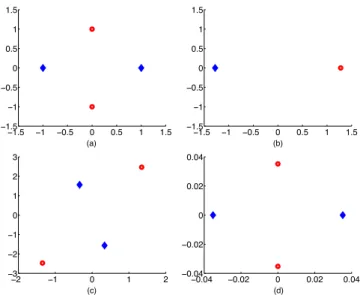
A main reason for the popularity of linear metric learn-ing is its good off-the-shelf usability. However, linear met-ric learning has inherent limits on their mapping capability. Nonlinear metric learning is more general and offers greater separation ability in theory. For example, for the four points in two classes in Figure 1.a), no linear metric learning meth-ods can give correct kNN classification. For example, the lin-ear transformation in Figure 1.c) only rotates and scales the data, so does the LMNN mapping in Figure 1.d). We can see that kNN classification on the mapped data points in Figure 1.c) and 1.d) still cannot separate the two classes correctly. However, our nonlinear transformation (to be explained in Section 6.1) can map the four points to the coordinates in Figure 1.b), which enable correct kNN classification.

Nonlinear metric learning methods, although more expres-sive, are far less popular than linear methods. Often, they are not easy to use, since they require complex

(5)

!"# ! $"# $ $"# ! !"# !"# ! $"# $ $"# ! !"# !"# ! $"# $ $"# ! !"# !"# ! $"# $ $"# ! !"# ! " # " ! $ ! " # " ! $ !"!# !"!$ ! !"!$ !"!# !"!# !"!$ ! !"!$ !"!# (a) (b) (d) (c)

Figure 1: An toy example with four points in two

classes, marked in different shapes. a) shows the orig-inal data; b) shows the data after our KDML mapping (the two points in each class are very close to each other); c) shows a random linear transformation; d) shows the data after LMNN mapping.

tion, not only for coefficient training, but also for model selection and hyper-parameter tuning. For example, kernel-ization methods [3,7,12,21] are inherently limited by the size of the kernel matrices. Neural network based methods [4] are also very expensive. Furthermore, these nonlinear methods often require tuning of many hyper-parameters. Their sensi-tivity to the parameter tuning further hinders their off-the-shelf usability, especially for unknown domains. Recently, Kedem et al. proposed two nonlinear metric learning algo-rithmsχ2-LMNN and GB-LMNN [13]. χ2-LMNN still uses the linear transformation in (1) but employs a non-Euclidean distance. However,χ2_{-LMNN has rather limited scope: it}

can only be applied when the input data are sampled from a simplexSD₌_{_x_{∈ R}D_|_x_≥₀_,_xT₁_{= 1}_}_{. GB-LMNN learns}

a nonlinear mappingφ(x) which is an ensemble over a num-ber of regression trees with different heights. GB-LMNN applies gradient boosting to learn the nonlinear mapping in a function space.

In this paper, we propose a new metric learning framework calledkernel density metric learning (KDML). It uses kernel density regression to nonlinearly map each attribute to a new feature space. The distance is then defined as the Euclidean distance in the new space. Although we focus on integrating KDML with LMNN in this paper, this nonlinear metric learning framework is general and can be used to support many other metric learning algorithms such as NCA and ITML.

There are several salient advantages of the KDML ap-proach. 1) It embodies excellent nonlinear distance mea-sures with a sound probabilistic explanation. In fact, the Euclidean distance in the mapped feature space corresponds to established distance measures between probability den-sity functions. As a result, such nonlinear mapping allows us to correctly classify datasets that are notoriously difficult to tackle by linear metric learning methods. 2) Compared

to kernel-based nonlinear metric learning methods, KDML is easier to use and offers good off-the-shelf usability. In fact, end users do not need to tune any parameter in KDML since we can automatically learn its hyper-parameters using gradient descent. Moreover, KDML can be used as a pre-processing blackbox to map features and be integrated with any supervised metric learning algorithm. Thus, it allows us to leverage the extensive development on efficient and scal-able linear metric learning methods. 3) Unlike most existing metric learning methods which require the attributes to be numerical, KDML is the first metric learning algorithm that can naturally handle both numerical, categorical, and mixed attributes in a unified fashion.

This paper contains the following contributions. We in-troduce KDML, a nonlinear metric learning algorithm, by proposing a novel nonlinear mapping which provides a good similarity measure based on kernel density estimation. It can naturally handle both numerical and categorical features and offers good out-of-the-box usability. Further, we inte-grate KDML with LMNN, and develop an optimization algo-rithm to train the model in a holistic way. The algoalgo-rithm au-tomatically finds optimal bandwidths for a Nadaraya-Watson kernel density estimator, which is absent in previous work. Finally we conduct extensive evaluation on a collection of datasets for multiway classification, with both numerical and categorical features. We show that KDML improves the performance of state-of-the-art metric learning methods for kNN classification tasks.

The rest of this paper is organized as follows. Section 2 gives some preliminaries for metric learning. Section 3 presents the proposed KDML model, including its nonlin-ear mapping and kernel density estimation. Section 4 com-bines KDML with LMNN and presents the optimization algorithm for learning the transformation matrix and ker-nel bandwidths. Section 5 surveys related work on metric learning. Section 6 presents experimental results of different metric learning algorithms on various benchmark datasets. Finally, Section 7 gives conclusions and discusses our future work.

2. PRELIMINARIES

In this paper, we focus on a supervised classification set-ting. The main ideas can also be extended to other settings such as weakly supervised, semi-supervised, or unsupervised ones.

We assume we are given a training data set

T ={(x1, y1),· · ·,(xN, yN)} ∈ D1× · · · × DD× C, (2)

where there thedth_{feature is defined in a domain}_D d and

the label yi’s are from a set of C classes C = {1,· · ·, C}.

Note that our setting is more general than typical previous settings, because the domain Di can either be a numerical

set such asRor a categorical set.

We use large-margin nearest neighbors (LMNN) [22] as the basic metric learning method to be integrated with KDML. We briefly review the basics of LMNN here.

LMNN is a linear metric learning algorithm that is tai-lored for kNN classification. For each new input x, kNN classifies x by a majority vote from the k neighbors that are closest toxunder a certain distance metric. Therefore, kNN classification relies heavily on the distance metric and provides a most natural paradigm for evaluating various dis-tance metric learning algorithms.

(6)

LMNN uses the linear transformation in (1). Equivalently, it learns a Mahalanobis distance:

d2M(xi,xj) = (xi−xj)TM(xi−xj), (3)

whereM=LTLis a positive semi-definite matrix.

In LMNN, for each input (xi, yi), it specifies a number of

target neighborswith the same label asyi. Normally thesem

target neighbors are simply themneighbors with the same label that are closest toxibased on the Euclidean distance.

We use j ; i to denote that xj is a target neighbor of

xi, andyij∈ {0,1}to denote whether the labelsyjand yi

match (yij= 1 whenyi=yj).

The objective function of LMNN is to minimize

E(M) = (1−µ) X i,j;i d2_M(xi,xj) + µ X i,j;i,l (1−yil)1 +d2M(xi,xj)−d2M(xi,xl)₊ (4) where [z]+ = max(0, z) is the standard hinge loss and µ∈

(0,1) is a positive constant controlling the relative weights of the two terms. The first term minimizes the distance be-tween each input and its target neighbors, and the second term, incorporating the idea of a margin as in SVM, pe-nalizes the distances between those mismatched points that “invade” the neighborhood of each input.

It is shown that the optimization in (4) can be reformu-lated into a semidefinite program (SDP) [22]. Weinberger et al. have proposed a specialized subgradient descent algo-rithm to solve this SDP, by exploiting the sparsity of active invaders in the second term of (4). LMNN has received great attention and popularity due to its good kNN classification performance, efficiency, and easiness to use.

Another important work is the information-theoretic met-ric learning (ITML) [5]. ITML also uses the linear trans-formation in (3) but utilizes a one to one correspondence between the Mahalanobis distance parameterized byMand a multivariate Gaussian as P(x;M) = 1 Z exp(− 1 2d 2 M(x,x0)), (5)

whereZ is a normalization factor andx0is the mean of the Gaussian. Using this correspondence, the objective of ITML is to minimize

KL(p(x;M0)kp(x,M)) =

Z

p(x;M0) lnp(x;M0)

p(x;M)dx, whereM0is a fixed matrix suchIor the inverse covariance matrix. The intuition is to regularizeMby minimizing the Kullback-Leibler (KL) divergence [14] between the implied distributionP(x;M) and a prior distribution.

3. THE KDML FRAMEWORK

In this section, we propose the KDML framework for non-linear metric learning. We assume that we are given inputs (x, y)∈ D1× · · · × DD× C, where thedthfeature is defined

in a domainDd and the label y is from a set of C classes

C={1,· · ·, C}.

3.1 KDML feature mapping

Under the KDML framework, we propose two kinds of transformation for each input (x, y).

Density features. For each dimensiond = 1,· · ·, D and anyxd∈ Dd, there exists a conditional probability density

function

Pd(c, xd) =P(y=c|xd), c= 1,· · ·, C. (6)

We usePd(xd) to denote the vector [Pd(1, xd),· · ·, Pd(C, xd)].

In this transformation, each input is transformed into a vector

φP(x) = [P1(x1);· · ·;PD(xD)], (7)

which is a concatenation of all the D probability density vectors.

An alternative is to use the square roots of the probabili-ties.

Sd(c, xd) =

p

P(y=c|xd), c= 1,· · ·, C, (8)

which leads to a corresponding feature vectorφS(x).

Entropy features. For each dimensiond= 1,· · ·, Dand anyxd∈ Dd, we compute the logarithm of the density

Ed(c, xd) = lnP(y=c|xd), c= 1,· · ·, C. (9)

LetEd(xd) denote the vector [xEd(1, xd),· · ·, Ed(C, xd)].

In this mapping, each input is transformed into a vector

φE(x) = [E1(x1);· · ·;ED(xD)], (10)

which is a concatenation of all the entropy vectors.

In KDML, we choose a feature mapping fromφP,φS, and

φE and name it φ. We may also include the original

vari-ables in the feature vector to make it strictly more general than linear mapping. It then employs an existing linear met-ric learning method to learn a linear transformationLφ(x) which gives rise to a Mahalanobis distance in the mapped feature space.

3.2 Implied distance measures

We now discuss the distance measures implied by using the above KDML features. We can see that they all corre-spond to some sound distance/similarity measures between two probability density functions. As a result, in many cases, the Euclidean distance in the feature space after mapping re-flects a better distance measure than the Euclidean distance in the original input space.

One way to view KDML is that it first transforms the original input into a new space. In the new space, before any metric learning, the similarity between two data points are based on the Euclidean distance between their feature vectors:

d2(xi,xj) = (φ(xi)−φ(xj))T(φ(xi)−φ(xj)). (11)

In fact, since there are D dimensions, each data point corresponds toDprobability density functions (PDFs), each withC possible values. That is, for an inputxi, its PDF at

thedthdimension is

PDFi,d= [Pd(1, xi,d),· · ·, Pd(C, xi,d)], (12)

where we use xi,d to denote the dth attribute of xi. The

(7)

dimensions d2(xi,xj) = D X d=1 diff(PDFi,d,PDFj,d), (13)

where diff() measures the distance between two PDFs over the setC.

Distance or similarity measures between PDFs have been extensively studied. A good survey of these measures can be found in [2]. To justify the features in KDML, we examine the underlying distance measures they imply.

When the density feature φS is used, considering two

pointsxi andxj, their Euclidean distance is

d2(xi,xj) = (φS(xi)−φS(xj))T(φS(xi)−φS(xj)) = D X d=1 C X c=1 [p Pd(c, xi,d)− p Pd(c, xj,d)]2

Therefore, usingφSfeatures, the implied distance measure

between the PDFs is diffS(PDFi,d,PDFj,d) = C X c=1 [pPd(c, xi,d)− p Pd(c, xj,d)]2.

The above equation is exactly the well-known squared-chord PDF distance measure [8], which is also the square of the Matusita distance measure [15]. Hence, theφS feature

im-plies the squared-chord and Matusita PDF distance mea-sures.

When the density feature φP is used, considering two

pointsxi andxj, their Euclidean distance is

d2(xi,xj) = (φP(xi)−φP(xj))T(φP(xi)−φP(xj)) = D X d=1 C X c=1 [Pd(c, xi,d)−Pd(c, xj,d)]2. (14)

We can see that, usingφP features, the implied distance

measure between two PDFs is diffP(PDFi,d,PDFj,d) =

C

X

c=1

[Pd(c, xi,d)−Pd(c, xj,d)]2. (15)

We can see that (15) is exactly the commonly used squared Euclidean distance measure between two PDFs [2].

Furthermore, the well-known Squared χ2 _{PDF distance}

measure [18] is diffχ2(PDFi,d,PDFj,d) = C X c=1 [Pd(c, xi,d)−Pd(c, xj,d)]2 Pd(c, xi,d) +Pd(c, xj,d) (16) Comparing (15) with (16), we can see that diffχ2 can be obtained if we apply a linear transformation toφP(xi) and

φP(xi) (by dividing φP(d, c) by

p

Pd(c, xi,d) +Pd(c, xj,d))

and then use the Euclidean distance as the distance mea-sure. In this sense, the metric learning is more general since it learns a linear transformation M, in the entire space of positive semi-definite matrices. SinceM is learned under the guidance of some external objectives, such as optimiz-ing the kNN classification accuracy, we expect it to give better metric for each specific data mining task than the fixed transformation in the squaredχ2 _measure.

Finally, when the entropy feature φE is used, the

Eu-clidean distance between two pointsxiandxjis

d2(xi,xj) = (φE(xi)−φE(xj))T(φE(xi)−φE(xj)) = D X d=1 C X c=1 [lnPd(c, xi,d)−lnPd(c, xj,d)]2 = D X d=1 C X c=1 lnPd(c, xi,d) Pd(c, xj,d) 2 (17) Using φE features, the implied distance measure between

the PDFs is diffE(PDFi,d,PDFj,d) = C X c=1 lnPd(c, xi,d) Pd(c, xj,d) 2 , (18)

which is not a known PDF distance measure to our knowl-edge but embodies, under a linear transformation that can be reflected in the Mahalanobis matrix M, the following squared variant of KL divergence [14]

diffKL2(PDFi,d,PDFj,d) = C X c=1 Pd(c, xi,d) lnPd(c, xi,d) Pd(c, xj,d) 2

In summary, the proposed features correspond to some sound distance measures between two PDFs. We believe that they usually give a more reasonable distance measure than the original Euclidean distance. Performing metric learning on these transformed features may allow us to im-prove many learning algorithms.

3.3 Kernel density estimation for computing

features

We have proposed the feature mappingsφP,φS, andφE

for KDML. Now we estimate the conditional probability densities in these features. From (6), (8) and (9), all of them require estimatingP(y=c|xd), for eachxd∈ Dd and

c = 1,· · ·, C. Once we have all the P(y = c|xd), those

features can be computed.

Given training dataT ={xi, yi},i= 1,· · ·, N, We

parti-tionT intoCsubsetsT1,· · ·,TC, which contain data points

with labelsy= 1,· · ·, y=C, respectively.

To estimatep(y=c|xd), we distinguish the cases of

cat-egorical and numerical attributes. We use ˆp(y = c|xd) to

denote the estimates.

Categorical attributes. If an attributexdtakes

categor-ical values,p(y=c|xd) can be estimated by the proportion

of samples with y = c among all the samples whose dth

attribute isxd. Thus, it can be computed using:

ˆ p(y=c|xd) =|Tk T Txd| |Txd| , c= 1,· · ·, C (19) whereTxd={xi|xi,d=xd, i= 1,· · ·, N}is the set of

sam-ples inT whosedth attribute isxd.

Numerical attributes. If an attributexdtakes numerical

values, we propose to use a Nadaraya-Watson type kernel density regression to estimatep(y=k|xd), k= 0,1.

According to the Nadaraya-Watson estimator [1, 16], we have: ˆ p(y=c|xd) = P i∈TcK( xd−xi,d hd ) PN i=1K( xd−xi,d hd ) (20)

(8)

where K(x) is a kernel function satisfying K(x) ≥ 0 and

R

K(x)dx= 1, andhd >0 is a parameter called the

band-widthof the kernel density function. In this paper, we choose the Gaussian kernel forK(x), namely,

K(x) = √1

2πexp(− x2

2 ). (21)

We can thus compute the KDML features by substituting the estimates in (19) and (20) into (6), (8), and (9). For example, the entropy features for categorical and numerical attributes are, respectively,

Ed(c, xd) = ln |TcTTxd| |Txd| , (22) and, Ed(c, xd) = ln    P i∈Tcexp(− (xd−xi,d)2 2h2 d ) P i∈T exp(− (xd−xi,d)2 2h2 d )   . (23)

We also comment on the difference between the assump-tions of ITML and KDML. The main assumption of ITML is that all the data points are drawn from a single Gaussian distribution, centered at x0. Such an assumption may be too restrictive in some cases. KDML, in contrast, assumes a nonlinear distribution which is a mixture of multiple Gaus-sians at each dimension.

4. COMBINING KDML WITH LMNN

In principle, KDML is a general framework that can be combined with existing metric learning algorithms as a pre-processing step, which nonlinearly maps the features in the original space to a new space.

4.1 The KDML-LMNN approach

As a concrete application, we combine KDML with the LMNN algorithm and apply it to kNN classification. First, we map each training dataxinto a featureφ(x) (which may beφP(x),φS(x), orφE(x)). Then, we use LMNN to learn a

transformationLφ(x) which leads to a Mahalanobis distance

d2M(xi,xj) = (φ(xi)−φ(xj))TM(φ(xi)−φ(xj)), (24)

whereM=LTLis a positive semi-definite matrix.

Applying LMNN to φ(x), we solve the problem of mini-mizing: E(M) = (1−µ) X i,j;i d2M(xi,xj) + µ X i,j;i,l (1−yil) 1 +d2M(xi,xj)−d2M(xi,xl) +, (25) whered2 M(xi,xj) is defined in (24).

As a side note, we can also substituted2Min (24) into (5)

so that KDML is combined with ITML.

4.2 Optimization algorithm

The training of KDML-LMNN aims at learning the op-timal values of the matrix M and the bandwidths in the Nadaraya-Watson estimator. For each numerical attributes

xd, there is a hyper-parameter hd that needs to be

cho-sen. One way to choosehdis to use rules-of-thumb to set a

heuristichdvalues. A popular one is the Silverman’s rule of

thumb [20]:

h∗

d= 1.06σN−1/5, (26)

whereσis the standard deviation ofxd.

Although such rules-of-thumb often give solid performance, we can in fact derive a novel way to automatically choose optimalhdbased on the KDML-LMNN objective. Such

au-tomatic tuning is absent in previous work. We propose to find the hd that minimizes E in (25). For this

minimiza-tion, a nice fact is that we can get the closed form of the subgradient ∂E

∂hd and compute it efficiently.

There are two terms in (25). Let

E1= X i,j;i D_M2 (xi,xj), and (27) E2= X i,j;i,l (1−yil)1 +D2M(xi,xj)−D2M(xi,xl)₊ (28) We have E(M) = (1−µ)E1+µE2 (29)

We compute the gradients for these two terms separately. First, since ∂D2 M(xi,xj) ∂xi =∂D 2 M(xi,xj) ∂xi =M(xi−xj) (30) we have ∂E1 ∂xk =X j;k M(xk−xj) + X k6=j,k;j M(xk−xj). (31)

For E2, note that ∂E_∂_x2

k is a subgradient since it involves

a hinge loss and it is non-differentiable whenever the term inside [.]+ is zero. Therefore: when

[1 +D2_M(xi,xj)−DM2 (xi,xl)]<0, (32) ∂E₂ ∂xk is 0; otherwise, we have: ∂E2 ∂xk = X k,j;k X l (1−ykl)M(xl−xj) + X i6=k,k;i,l (1−yil)M(xk−xi) − X i,k;i (1−yik)M(xk−xi) (33)

Then, according to (29), ford= 1,· · ·, D, we have

∂E ∂hd = X k (1−µ)∂E1 ∂xk +µ∂E2 ∂xk T _∂_x k ∂hd (34) where ∂xk ∂hd = h 0,· · ·,∂φc,d(xk) ∂xk ,· · ·,0 iT is a column vector, where φc,d(xk) is the KDML feature value for the dth

di-mension and classcofxk. Use the entropy feature in (9) as

an example, we know φc,d(xk) = ln    P i∈Tcexp(− (xk,d−xi,d)2 2h2 d ) P i∈Texp(− (xk,d−xi,d)2 2h2 d )   . (35)

(9)

Algorithm 1Optimization for KDML-LMNN learning 1: Initializehusing (26)

2: repeat

3: compute the feature matrixΦh

4: call LMNN to optimizeM ⊲under fixedh&Φh

5: ford= 1to Ddo ⊲under fixedM

6: if xdis a numerical variablethen

7: hd←hd−γ_∂h∂E d ⊲gradient descent 8: end if 9: end for 10: until hconverges 11: outputhandM We now compute ∂φc,d(_∂hxk) d . Letrd=−1/(2h 2 d), we have: ∂φc,d(xk) ∂rd = P i∈Tc[(xk,d−xi,d) 2_·_exp(_r d(xk,d−xi,d)2)] P i∈Tcexp(rd(xk,d−xi,d) 2₎ − P i∈T[(xk,d−xi,d) 2_·_exp(_r d(xk,d−xi,d)2)] P i∈Texp(rd(xk,d−xi,d)2) (36) and ∂φc,d(xk) ∂hd = 1 h3 d ∂φc,d(xk) ∂rd . (37) Summarizing things together, we can get the closed form of ∂E

∂hd by assembling (34), (31), (33), (36), and (37). The

closed form of ∂E

∂hd seems complex but in fact can be

effi-ciently computed. ∂E

∂hd has two parts,

∂E1 ∂hd and ∂E2 ∂hd. ∂E1 ∂hd

has a simple form and only involves pairs of neighboring points satisfyingj;kork;j.

For ∂E2

∂hd, it is important to note that it is a

subgradi-ent. ForE2 in (28), for each pointi, we only need to

con-sider those “active”lthat are invading the neighborhood of

iso that the corresponding [.]+ term is positive. There are

typically few invaders. This is observed and exploited in LMNN to speed up its gradient computation [23]. In [23], it is found that thektarget neighbors and the invaders do not change frequently over each iteration. The LMNN package maintains such information in a data structure for efficient updates during the optimization process. This data struc-ture is adapted in our implementation to support efficient computation of ∂E

∂hd.

Lethto the vector of all thosehdfor numerical attributes

xd, d= 1,· · ·, D. We show our optimization algorithm for

training KDML+LMNN in Algorithm 1. It contains two levels of optimization: an outer loop which optimizeshusing subgradient descent, and an inner loop which learnsMusing the original LMNN package under fixedh.

In the outer level, at each iteration, the feature matrix

Φhcomposed ofφc,d(xk) is updated based on the newh. If

a variablexi is categorical, its feature is computed by (19).

For a numerical variablexd, we use the kernel density

esti-mation in (20) to compute its feature. Then, entering the inner level, we use the original LMNN package to learn the

Mthat minimizesE(M) in (25) under fixedhandΦh.

Fi-nally, we optimizehfor numerical attributes by performing descent along the subgradient direction in (34) based on the validation set. We use a line search with the Armijo rule to choose the step sizeγ.

As Algorithm 1 learnsMandh, there are no other hyper-parameters to tune for KDML-LMNN.

5. RELATED WORK

A number of prior works on metric learning have focused on learning a linear transformation in the original input space [5, 9, 11, 19, 23, 24]. They achieved great success in improving the performance of learning algorithms by ob-taining better Mahalanobis distance measures. The concept of distance metric learning was first proposed by Xing et al. [24]. Their objective is to learn a Mahalanobis matrix such that similar points are clustered together subject to the constraints that distances between dissimilar points are larger than a lower bound. Inspired by this general idea, many works have been developed.

LMNN [23] identifies the local target neighbors in the orig-inal space for each point and learns a Mahalanobis matrix such that the non-target neighbors for each point are en-couraged to be far away from all its target neighbors with a large margin. ITML [5] assumes that there exists a bijec-tion between the Mahalanobis distance and a single multi-variate Gaussian distribution. It minimizes the KL diver-gence between a prior distribution and the distribution im-plies by the Mahalanobis distance, subject to upper bound constraints on the distance between similar points and lower bound constraints on the distance between dissimilar points. The SEPAPH [17] approach also relies on a mapping from the Mahalanobis distance to a probability distribution but extends to semi-supervised metric learning based on regu-larization.

Neighborhood components analysis (NCA) [11] maximizes a softmax function that smooths the leave-one-out accuracy of kNN classification. However, it has a nonconvex objective function and suffers from local minima. Maximally collaps-ing metric learncollaps-ing (MCML) [9] constructs a convex objec-tive based on the same softmax function to characterize the distribution. It minimizes for each point the KL divergence between a “bi-level” distribution and the desired distribution under the Mahalanobis distance, where the bi-level distri-bution is zero for similar points and non-zero for dissimilar points.

All the above methods look for a linear transformation. However, the linearly transformed features fail to have sat-isfactory expression on many cases, such as the example in Figure 1. Another example is the case when the two classes of data form two concentric circles [23], which we will illus-trate in Section 6. Hence, there are also work on nonlinear distance metric learning.

One nonlinear extension is to kernelize existing methods and use the Representer’s Theorem to represent the nonlin-ear transformation using the kernel matrix elements [3, 10, 21]. However, these methods have not replicated the success of linear methods and out-of-the-box packages based on such kernelization are lacking. In general, direct kernel methods are sensitive to hyper-parameters and their utility is limited inherently by the sizes of kernel matrices [13].

Another nonlinear approach, MM-LMNN [23], uses mul-tiple metrics for different clusters of data to achieve global nonlinearity, where the clusters are obtained by thek-means algorithm. However, the transformation is locally linear with respect to each cluster and the cross-cluster distances cannot be easily learned. Two other nonlinear methods are proposed in [13]. χ2_{-LMNN uses a nonlinear} _χ2 _distance

(10)

!" # " # !" !" # " # !" ! " # $ % &' $ ' $ &' ! " ! #" $ " $ % & ' !"# ! $"# $ $"# ! !"# !"# ! $"# $ $"# ! !"# ! " # $ % !& % & % !&

(a) original data (b) iteration 1 (c) iteration 2

(e) iteration 4 (d) iteration 3

error:100% error:45% error:16%

error:13% error:0%

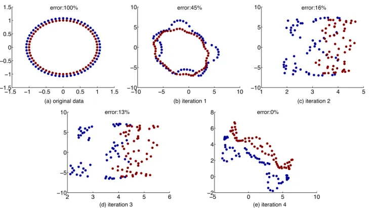
Figure 2: A toy example with two circles in two classes, marked in different colors. a) shows the original data; b) - e) show the data mapping and kNN classification error after each outer-loop iteration of Algorithm 1 which tunes h. The classification error quickly decreases to zero as h is optimized using subgradient descent.

measure. It is intended for histogram data and can only be applied when all the data lie on a simplexSD ₌_{_x _∈

RD|x ≥0,xT1 = 1}. KDML has much wider applicabil-ity thanχ2_{-LMNN since it can process any input, into}

his-tograms for categorical data and probability densities for numerical data. GB-LMNN uses a set of gradient boost-ing regression trees with different heights and optimizes the objective function of LMNN. GB-LMNN is shown to per-form better than its linear counterpart LMNN and MM-LMNN [13].

6. EXPERIMENTAL RESULTS

We conduct extensive experiments to evaluate the KDML-LMNN approach in Algorithm 1, or KDML for short in this section. We evaluate KDML withφP, φS, or φE features

(denoted as KDMLP, KDMLS, and KDMLE, respectively).

Note that KDML can be applied to datasets with numerical, categorical, and mixed attributes.

For comparison, we also evaluate two state-of-the-art lin-ear metric llin-earning algorithms including LMNN [22] and ITML [5]. We also evaluate a nonlinear metric learning algo-rithm MM-LMNN [23], which first groups data into clusters and then uses multiple linear mappings for different clusters to achieve globally nonlinear mapping. Both LMNN and MM-LMNN are obtained from their website1. ITML code is obtained from http://www.cs.utexas.edu/∼pjain/itml/. We also evaluate using the original Euclidean distance as a baseline.

We implemented the KDML algorithm inside the LMNN

1_{http://www.cse.wustl.edu/}_∼_{kilian/code/lmnn/lmnn.html}

package, which is implemented in Matlab. For full replicabil-ity of the experiments, our KDML code is made available on-line at http://www.cse.wustl.edu/∼chen/kdml/. All exper-iments are performed on a desktop computer with 2.67GHz CPU and 8G memory running Mac OS X 10.7.

6.1 Illustrations on toy cases

For sanity check and illustration, we first test on a simple example in Figure 1a). This data cannot be correctly sepa-rated by any linear metric learning algorithm. Since KDML maps the data to a higher dimensional space, to visualize the mapping in 2-D, we extract a 2-D transformationL∈ R2×D

fromMusing eigendecomposition. Such dimensionality re-duction is in fact another main utility of metric learning and already implemented in LMNN. Figure 1b) shows the 2-D mapping result by KDML, which clearly separates the two classes. Figures 1c) and 1d) show that linear transforma-tions cannot separate the two classes.

We also test another toy example shown in Figure 2a). It contains two concentric circles of data from two different classes. It is a very difficult case since the nearest neigh-bor of any given data point is from the other class. It is a well-known example as no linear transformation can sepa-rate these two classes [13].

Figures 2b) to 2e) illustrate the process of KDML-LMNN in Algorithm 1 which automatically tunes the kernel band-widthh. For better visualization, the results in Figures 2b) to e) are obtained by applying Algorithm 1 and extract-ing a 2-D mappextract-ing usextract-ing eigendecomposition of Mat each outer-loop iteration. We can see that the kNN classification error quickly decreases from 45% after the initial KDML

(11)

Type Dataset N C Dn Dc

Numerical Glass_Wine 214₁₇₈ 7₃ 10₁₃ 0₀ Mixed Contraceptive_{Statlog Heart} 1473₂₇₀ 3₂ 2₆ 7₇ Categorical

Hayes-Roth 160 3 0 5

Balance Scale 625 3 0 4

Car 1728 4 0 6

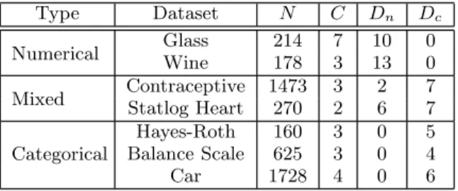
Table 1: The number of instances N, number of

classes C, number of numerical features Dn, and

number of categorical featuresDc of the tested UCI

datasets.

mapping to 0% in just four major iterations of optimizingh

using subgradient descent.

6.2 Results on numerical datasets

We test all the algorithms on benchmark datasets from the UCI repository [6]. We choose datasets mostly with multiple (≥3) classes since kNN has salient advantages over other methods such as SVM on multiway classification. For each dataset, we run a 10-fold cross validation with 90/10 splits and report the average results. We usek= 3 for kNN classification on all the cases.

Table 1 lists the main characteristics of the tested datasets. We can see that there are datasets with numerical, categor-ical, and mixed attributes.

Table 2 compares kNN classification errors of various al-gorithms on the numerical datasets. We observe that all KDML algorithms, with three different kinds of feature map-pings, consistently perform significantly better than other algorithms in most cases.

6.3 Results on categorical and mixed datasets

Another major advantage of KDML is its ability to natu-rally handle categorical variables. We also evaluate our al-gorithms on datasets with categorical attributes and mixed data types from the UCI repository.

To deal with a categorical attributex, KDML transforms

xinto numerical features defined asφP(x),φS(x) orφE(x)

before. For other algorithms, we use a typical multinomial encoding to handle categorical variables. For each categori-cal attributexthat hasmdifferent categories, we transform it intomnumbers with only one of the numbers being 1 and the others being 0.

Table 2 also lists the kNN classification results on datasets with categorical attributes. We observe that all KDML al-gorithms, with different features, again consistently perform much better than other algorithms on all the cases. KDMLE

is the overall winner with the best performance on all the categorical and mixed datasets, except for the Statlog Heart dataset where it is only slightly (well within one standard error) worse than ITML.

7. CONCLUSIONS AND FUTURE WORK

In this paper, we have proposed a novel kernel density metric learning (KDML) framework for nonlinear distance metric learning. KDML is fundamentally different from the previous metric learning algorithms since it introduces a nonlinear mapping from the original input space into a prob-ability density space, based on Nadaraya-Watson kernel

den-sity estimation. We have shown that the nonlinear mapping in KDML embodies established distance measures between probability density functions, and leads to correct classifi-cation on datasets on which linear metric learning methods would fail. KDML can be used as a preprocessing step and combined with existing metric learning algorithms. We have integrated KDML with the LMNN algorithm. Under this framework, we have derived the closed form of the subgra-dients of the objective function with respect to the kernel bandwidths. We have then derived an integrated optimiza-tion algorithm for learning the Mahalanobis matrix and ker-nel bandwidths. Extensive results on real-world numerical and categorical data show that, KDML gives significantly better kNN classification quality than other linear and non-linear metric learning algorithms. Unlike previous metric learning algorithms, KDML can naturally handle both nu-merical and categorical data. It is also easy to use and offers good off-the-shelf usability. These advantages make KDML an attractive general approach for metric learning.

Our ongoing work is focused on combining the nonlinear features in KDML with more expressive parametric forms of the distance function such as that inχ2_{-LMNN and}

KL-divergence, instead of the simple Euclidean ℓ2 form. The

flexibility in both feature mappings and distance functions may enable us to construct superior distance/similarity mea-sures for a wide range of applications.

Acknowledgment

This work is partially supported by the CNS-1017701 and CCF-1215302 grants from the National Science Foundation of the United States, a Microsoft Research New Faculty Fel-lowship, and a Barnes-Jewish Hospital Foundation grant.

8. REFERENCES

[1] C. M. Bishop.Pattern Recognition and Machine Learning. Springer-Verlag New York, Inc., Secaucus, NJ, USA, 2006.

[2] S. H. Cha. Comprehensive survey on

distance/similarity measures between probability density functions.International Journal of Mathematical Models and Methods in Applied Sciences, 1:300–307, 2007.

[3] R. Chatpatanasiri, T. Korsrilabutr,

P. Tangchanachaianan, and B. Kijsirikul. A new kernelization framework for mahalanobis distance learning algorithms. Neurocomput.,

73(10-12):1570–1579, June 2010.

[4] S. Chopra, R. Hadsell, and Y. LeCun. Learning a similarity metric discriminatively, with application to face verification. InProceedings of the 2005 IEEE Computer Society Conference on Computer Vision and Pattern Recognition (CVPR’05) Volume 1 -Volume 01, CVPR ’05, pages 539–546, Washington, DC, USA, 2005. IEEE Computer Society.

[5] J. V. Davis, B. Kulis, P. Jain, S. Sra, and I. S. Dhillon. Information-theoretic metric learning. In

Proceedings of the 24th international conference on Machine learning, ICML ’07, pages 209–216, New York, NY, USA, 2007. ACM.

[6] A. Frank and A. Asuncion. UCI machine learning repository, http://archive.ics.uci.edu/ml, 2010.

(12)

Data set Euclidean ITML LMNN MM-LMNN KDMLP KDMLS KDMLE Glass 32.25±5.08 32.75±10.17 30.39±4.47 29.48±8.69 22.45±4.93 26.16±7.56 28.03±6.32 Wine 28.63±3.33 6.14 ±4.94 3.33±3.04 3.92±3.15 4.51±3.20 3.95±3.21 2.84±2.86 Contraceptive 51.19±3.03 51.33±3.39 50.65±1.81 52.41±3.66 50.37±2.27 50.44±2.53 50.37±3.34 Statlog Heart 38.15±7.81 22.22±8.38 24.44±4.22 26.30±6.85 25.56±1.55 26.67±4.46 22.96±3.84 Hayes-Roth 32.50±3.56 19.38±6.01 21.88±7.97 18.13±4.07 18.75±3.13 18.13±2.61 17.50±1.71 Balance Scale 28.80±2.99 18.40±4.42 21.76±3.94 12.64±10.33 17.12±2.44 14.56±2.22 10.88±2.81 Car 15.92±2.17 13.96±6.52 3.12±1.25 3.30±1.04 3.13±1.24 3.30±0.79 3.07±0.93 Table 2: KNN classification error (in %, ± standard deviation) of various methods on the UCI datasets, averaged over 10-fold 90/10 training-testing splits. Best results are shown in bold.

[7] C. Galleguillos, B. McFee, S. J. Belongie, and G. R. G. Lanckriet. Multi-class object localization by combining local contextual interactions. InCVPR, pages 113–120. IEEE, 2010.

[8] D. Gavin, W. Osward, E. Wahl, and J. Williams. A statistical approach to evaluating distance metrics and analog assignments for pollen records. 60:356–367, 2003.

[9] A. Globerson and S. Roweis. Metric learning by collapsing classes. InProc. NIPS, 2005.

[10] A. Globerson and S. T. Roweis. Visualizing pairwise similarity via semidefinite programming.Journal of Machine Learning Research - Proceedings Track, 2:139–146, 2007.

[11] J. Goldberger, S. Roweis, G. Hinton, and R. Salakhutdinov. Neighbourhood components analysis. InProc. NIPS, pages 513–520, 2004. [12] P. Jain, B. Kulis, J. V. Davis, and I. S. Dhillon.

Metric and kernel learning using a linear transformation.Journal of Machine Learning Research, 13:519–547, 2012.

[13] D. Kedem, S. Tyree, K. Weinberger, F. Sha, and G. Lanckriet. Non-linear metric learning. InProc. NIPS, 2012.

[14] S. Kullback and R. Leibler. On information and sufficiency.Ann. Math. Statist., 22:79–86, 1951. [15] K. Matusita. Decision rules, based on the distance, for

problems of fit, two samples, and estimation.Ann. Math. Statist., 26:631–640, 1955.

[16] E. Nadaraya. On estimating regression.Theory of Probability and its Applications, 9:141–142, 1964. [17] G. Niu, B. Dai, M. Yamada, and M. Sugiyama.

Information-theoretic semi-supervised metric learning via entropy regularization. InProceedings of the 29th international conference on Machine learning, ICML ’12, 2012.

[18] K. Pearson. On the criterion that a given system of deviations from the probable in the case of a correlated system of variables is such that it can be reasonably supposed to have arisen from random sampling.Phil. Mag., 50:157–172, 1900.

[19] N. Shental, T. Hertz, D. Weinshall, and M. Pavel. Adjustment learning and relevant component analysis. InProceedings of the 7th European Conference on Computer Vision-Part IV, ECCV ’02, pages 776–792, London, UK, UK, 2002. Springer-Verlag.

[20] B. W. Silverman and P. J. Green.Density Estimation for Statistics and Data Analysis. Chapman and Hall, 1986.

[21] L. Torresani and K. chih Lee. Large margin component analysis. In B. Sch¨olkopf, J. Platt, and T. Hoffman, editors,Advances in Neural Information Processing Systems 19, pages 1385–1392. MIT Press, Cambridge, MA, 2007.

[22] K. Weinberger, J. Blitzer, and L. Saul. Distance metric learning for large margin nearest neighbor classification. InProc. NIPS, 2005.

[23] K. Weinberger and L. Saul. Distance metric learning for large margin nearest neighbor classification.

Journal of Machine Learning Research, 10:207–244, 2009.

[24] E. P. Xing, A. Y. Ng, M. I. Jordan, and S. J. Russell. Distance metric learning with application to clustering with side-information. InProc. NIPS, pages 505–512, 2002.