O
N
C
OMPARING THE
A
CCURACY OF
D
EFAULT
P
REDICTIONS IN THE
R
ATING
I
NDUSTRY
WALTER KRÄMER
ANDRÉ GÜTTLER
CESIFO WORKING PAPER NO. 2202
C
ATEGORY10:
E
MPIRICAL ANDT
HEORETICALM
ETHODSJ
ANUARY2008
An electronic version of the paper may be downloaded
• from the SSRN website: www.SSRN.com
• from the RePEc website: www.RePEc.org
CESifo Working Paper No. 2202
O
N
C
OMPARING THE
A
CCURACY OF
D
EFAULT
P
REDICTIONS IN THE
R
ATING
I
NDUSTRY
Abstract
We consider 1927 borrowers from 54 countries who had a credit rating by both Moody's and S&P at the end of 1998, and their subsequent default history up to the end of 2002. Viewing bond ratings as predicted probabilities of default, we consider partial orderings among competing probability forecasters and show that Moody's and S&P cannot be ordered according to any of these. Therefore, the relative performance of the agencies depends crucially on the way in which probability predictions are compared.
JEL Code: C40, C53.
Keywords: credit rating, probability forecasts, calibration.
Walter Krämer Statistics Department University of Dortmund 44221 Dortmund Germany [email protected] André Güttler Finance Department University of Frankfurt 60325 Frankfurt Germany Version August 2007
Research supported by Deutsche Forschungsgemeinschaft (DFG) under SFB 475.We are grateful to Mark Wahrenburg, Jan-Pieter Krahnen, Martin Weber, Atanasios Mitropoulos and two anonymous referees for helpful criticism and comments.
1
Introduction
The evaluation of the quality, in whichever way defined, of default predictions in the credit industry has received considerable attention recently (Carey 2002, Engelmann et al. 2003 and many others). In particular, there is a growing interest in comparing the accuracy of competing rating agencies, or to rate the raters, so to speak. In the wake of Basel II, there will be a rapidly increasing number of rating producers, in addition to the established rating agencies, and an increasing number of borrowers who are rated by at least two of them, so it is natural to ask: which rater rates best?
This question can be answered in a variety of ways. The most popular method is based on the accuracy ratio, i.e. on how successful a rating system is in bucketing the defaults in the ”bad” grades, or its equivalent, the area under the ROC-curve (see section 4 or Sobehard and Keenan 2001 for a convenient introduction). A rating system is optimal in this sense if its worst grades end up with comprising all the defaults, and none of the non-defaults, i.e. if all defaults are rated worse than non-defaults. What is exactly meant by attaching one of the worst grades to a particular debtor is of no importance here, what matters is simply that debtors who later on default are considered riskier than debtors who do not default.
Below, we follow a different approach by viewing ratings as predicted probabili-ties of default, and by comparing the accuracy of these predictions across rating agencies. In doing so, we borrow heavily from mathematical statistics, where the evaluation of probability forecasts has a long and distinguished history (see e.g. DeGroot and Fienberg 1983, Vardeman and Meeden 1983, DeGroot and Eriksson 1985, or Winkler 1994, 1996). So far, this methodology has mostly been applied to weather forecasts (i.e. forecasts of the probability of rain) but it can easily be extended to default predictions in the rating industry.
The practical relevance of this exercise is obvious: The Basel II agreement will leave banks no choice but be attach predicted probabilities of default to all outstanding dept, so the ability to judge the quality of probability forcasts will be essential both for the banking business and for investors as well. If one could show, for instance, that one rater is better able to predict probabilities of default than another one, then its ratings should be more influential as concerns the yields of bonds rated by both of them, not to mention the ability to require higher fees.
As an example, we consider 1927 borrowers, mostly industrial firms and finan-cial institutions from the US (68 % of all borrowers), who had a credit rating by both Moody’s andS&P as of Dec. 31, 1998. We follow these firms up to the end of 2002 and record all defaults. The data were obtained from Bloomberg and are available from the authors on request.
Below we apply various orderings of probability forecasts to this data set. As these orderings are scattered in the statistics literature, we start by col-lecting and briefly reviewing them in section 2. Section 3 is concerned with mapping rating grades to probabilities of default, and section 4 compares the performance of the ratings, both in terms of partial orderings and in terms of various scalar measures of performance which have been suggested in the liter-ature. Section 5 addresses the statistical significance of the observed differences in performance, and a brief discussion of the shortcomings of our analysis in section 6 concludes.
2
Partial orderings of probability forecasts
Let 0 = a1 < a2 < . . . < ak = 1 be k predicted probabilities of default. In
practice, k varies from 6 to about 20. The US-based Loan Pricing Corporation hask= 10. The rating agencies which concern us in the present paper, Moody’s
andS&P, both have scales withk = 21 (taking account of modifiers such as + and - or 1, 2 and 3). For ease of comparability with these established agencies, most commercial banks also employ scales with k = 21 in their post Basel II internal rating systems.
Below we take the mechanism employed for the predictions as given. Produc-ing the predictions is a separate problem which has engendered an enormous literature, but will not concern us here. Rather, our point of departure is the discrete bivariate probability function r(θ, aj); θ = 0,1; j = 1, ..., k, resulting
from some such method, whichever it may be, with θ = 1 indicating default and θ = 0 indicating non-default.
The following additional notation will be used:
p(1) :=Pjr(1, aj) = overall relative frequency of default.
p(0) :=Pjr(0, aj) = overall relative frequency of no default.
q(aj) := relative frequency with which default probability forecast
aj is made.
p(1|aj) := rq(1(a,ajj)) = conditional relative frequency of default given
probability forecast aj.
p(0|aj) := rq(0(a,ajj)) = conditional relative frequency of no default
given probability forecast aj.
q(aj|1) := r(1p(1),aj) = conditional relative frequency of predicted
de-fault probability aj given default.
q(aj|0) := r(0p(0),aj) = conditional relative frequency of predicted
de-fault probability aj given no default.
The problem is: given two forecasters A and B, characterized by their re-spective bivariate probability functions rA(θ, a
j) and rB(θ, aj), which one is
One sensible requirement is that among borrowers with predicted default prob-ability aj, the relative percentage of defaults will be roughly equal toaj.
For-mally:
aj =! p(1|aj) = r(1, aj)
q(aj)
whenever q(aj) > 0. Such forecasters are called ”well calibrated” (DeGroot
and Fienberg 1983).
However, calibration, though desirable, is not sufficient for a useful forecast. For instance, a probability forecaster attaching default probability p(1) to all borrowers is well calibrated but otherwise quite useless.
Let rA(θ, a
j) and rB(θ, aj) be the joint probability functions of forecasters
A and B, respectively, with a nondegenerate marginal distribution p(θ). We assume that this marginal distribution is the same for both forecasters, i.e. that both agencies rate the same set of borrowers. First, we confine ourselves to forecasters which are both well calibrated. Following DeGroot and Fienberg (1983), we say that A is more refined than B, in symbols: A ≥R B, if there
exists a k×k Markov matrix M (i.e. a matrix with nonnegative entries whose columns sum to unity) such that
qB(a i) = k X j=1 MijqA(aj), and (1) aiqB(ai) = k X j=1 MijajqA(aj), i= 1, . . . , k. (2)
Equation (1) means that, given A’s forecast aj, an additional independent
randomisation is applied according to the conditional distribution Mij (j =
1, ..., k) which produces forecasts with the same probability function as that of B. Condition (2) ensures that the resulting forecast is again well calibrated. Table 1, from Kr¨amer (2003), provides an example. Forecaster A attaches a default probability of 2 % to all borrowers. If the overall default probability
is indeed 2 %, he is obviously well calibrated. Forecaster B is more refined; he attaches default probabilities 1 % and 3 %, respectively, to 50 % of all bor-rowers. We assume that he, too, is well calibrated. Likewise forecasters C and D with distributions across predicted default probabilities as given in the table.
Table 1:
The refinement ordering
among well calibrated probability forecasters forecast of distribution of borrowers across default probability predicted default probabilities
% A B C D 0.5 0 0 0.25 0.2 1 0 0.5 0 0.25 1.5 0 0 0.5 0 2 1 0 0 0 3 0 0.5 0 0.55 4.5 0 0 0.25 0
Obviously, B, C and D are more refined than A. Also, C and D are more refined than B: If all borrowers who receive a 0.5 % rating from C, and a randomly selected 50 % of those who receive a rating 1.5 %, are given a rating of 1 %, the rest a rating of 3 %, we obtain a new, well calibrated forecast with the same probabilistic properties as B’s.
The same can be done with D: All borrowers with ratings 0.5 % and 1 %, and a randomly selected one-eleventh of borrowers rated 3 %, are given a new rating of 1 %, the rest a new rating or 3 %. Again, this yields a new, well calibrated forecast with the same probabilistic properties as B’s.
On the other hand, C and D cannot be compared according to the refine-ment ordering. DeGroot and Fienberg (1983, Theorem 1) show that, for well calibrated forecasters A and B,
A≥R B ⇐⇒ j−1
X
i=1
(aj−ai)[qA(ai)−qB(ai)] ≥ 0, j=1,...,k-1. (3)
and this condition is violated for C and D in our example.
Vardeman and Meeden (1983) suggest to alternatively order probability fore-casters according to the concentration of defaults in the ”bad” grades. This will here be called the VM-default order. Formally:
A≥V M(d) B :⇐⇒ j X i=1 qA(ai|1) ≤ j X i=1 qB(ai|1), j=1,...,k. (4)
Or to put this differently: A dominates B in the Vardeman-Meeden default ordering if its conditional distribution, given default, first-order stochastically dominates that of B.
The same can be done for the non-defaults.Ais better thanB in the VM-non-default sense if non-VM-non-defaults are more frequent in the ”good” grades. Formally:
A≥V M(nd)B ⇐⇒ j X i=1 qA(ai|0) ≥ j X i=1 qB(ai|0), j=1,...,k. (5)
Finally, A dominates B in the Vardeman-Meeden sense (in symbols A≥V MB)
if both A≥V M(d)B and A≥V M(nd)B.
A final criterion which is favoured in the banking industry (see e.g. Falkenstein et al. 2000) is based on joining the points
(0,0), j−1 X i=0 q(ak−i), j−1 X i=0 q(ak−i|1) , j = 1, ..., k (6)
by straight lines. The resulting plot is variously called the power curve, the Lorenz curve, the Gini curve, or the cumulative accuracy profile, and a fore-casterAis considered better than a forecasterBin this - the Gini-default-sense (formally: A≥G(d)B) - ifA’s Gini curve is nowhere below that of B.
The Gini-curve would be diagonal if ratings were unrelated to defaults. There-fore, the area between the Gini-curve and the diagonal line can be viewed as measuring the quality of the forecasts – the larger the area, the better the fore-casts. This area, divided by the area obtained from forecasts where all defaults are rated worse than non defaults, is called the accuracy ratio; it is the most popular measure of forecasting performance in the banking industry.
3
Mapping rating grades to default
probabili-ties
Next, we apply the orderings described above to real world default predictions. Table 2 summarizes our data base. For each rating grade, it shows the number of debtors carrying this rating as of Dec. 31, 1998, and the number of defaults up to the end of 2002. There are 17 grades, with all debtors rated worse than
B- or B3 lumped together into grade C.
It is immediate from the table that there must be lots of split ratings. Dis-regarding the modifiers (i.e. the +0s and −0s attached by S&P and the 1,2,3
attached by Moody’s), there an 540 split ratings overall, with S&P ratings being better than Moody’s ratings in 359 cases and S&P ratings being worse than Moody’s ratings in 181 cases.
Table 2:
Distribution of borrowers across rating grades
S&P Moody’s
rating frequency number rating frequency number grade of defaults grade of defaults
AAA 55 0 Aaa 42 0 AA+ 33 0 Aa1 47 0 AA 80 0 Aa2 90 0 AA- 157 0 Aa3 142 0 A+ 167 1 A1 160 0 A 201 0 A2 191 2 A- 171 2 A3 154 0 BBB+ 170 3 Baa1 170 3 BBB 189 4 Baa2 180 1 BBB- 148 9 Baa3 165 9 BB+ 77 9 Ba1 69 6 BB 77 11 Ba2 50 2 BB- 85 26 Ba3 90 24 B+ 147 53 B1 76 19 B 106 49 B2 104 36 B- 43 25 B3 114 50 C 21 17 C 83 57 1927 209 1927 209
This percentage of split ratings corresponds to figures reported elsewhere, for instance in Ederington (1986). The reasons for such split ratings are a topic of independent interest and shall not concern us here. For instance split ratings might be an artefact of different procedures used for producing the ratings.
They may also occur because different raters have different standards of cred-itworthiness, or because raters which have the same standards simply disagree on the creditworthiness of a given debtor. See Ederington (1986) or Moon and Stotsky (1993) for a survey of such issues. As is shown in Ederington et al. (1987), bond ratings, both by Moody’s and S&P, do not incorporate the en-tirety of available information on the risk of default, so there is ample room for disagreement even if both agencies make the best use of information avail-able to them. Such issues certainly merit a lot of attention, but are outside the scope of the present paper. Rather, we first proceed under the assump-tions that (i) the true probabilities of default, given the rating grade, are the same for both agencies (where the correspondence between grades is as in table 2), and (ii) that the observed differences in empirical relative frequencies are due to random noise. This assumption will be later on relaxed. In addition, to obtain larger samples, we disregard the + and - modifiers and estimate the grade specific default probabilities by averaging the respective empirical relative frequencies from both agencies.
Column 3 in table 3 gives the results. It is seen that there were no defaults at all among the firms rated AAA or AA in the 1998 - 2002 period, with the first defaults occurring in grade A. Also, defaults are relatively more frequent, for a given letter grade, among debtors who had obtained that grade from S&P.
Columns 4 and 5 give the historical 4-year default frequencies as reported by the agencies themselves. They show that, apart from grades AAA and AA, the 4-year default rates in our sample are somewhat higher than the historical ones reported by the agencies themselves. The main reason is that our horizon covers the years 2001 and 2002, which saw an exceptionally large number of defaults: 70 of the 209 defaults in our sample occurred in 2001 and 58 occured in 2002. On the other hand the default rates reported by the agencies are averages of
18 (S&P) or 30 (Moody’s) four-year default horizons, covering various stages of the business cycle.
Table 3:
Empirical default probabilities (%) our sample historical Grade
Moody’s S & P average Moody’s S & P (1) (2) (3) (4) (5) AAA / Aaa 0 0 0 0.04 0.07 AA / Aa2 0 0 0 0.16 0.17 A / A2 0.40 0.56 0.48 0.36 0.48 BBB / Baa2 2.52 3.16 2.84 1.69 2.58 BB / Ba2 15.31 19.25 17.41 8.76 11.69 B / B2 35.71 43.20 39.32 27.04 27.83 C / C 68.68 73.91 71.15 55.05 51.25
On should note, however, that the rating agencies themselves are rather re-luctant to attach default probabilities to their letter grades. Or, to put it differently, the observed relative default frequencies should, strictly speaking, not be seen as probabilities of default predicted by the agencies. Both Moody’s and S & P for instance acknowledge that a letter grade of, say, AA, implies different probabilities of default in an economic downturn than in an economic upswing. In addition, ratings do not only incorporate default expectations but also expected loss, given default, so the relative frequencies in table 3 should only be viewed as rough indicators of predicted probabilities of default. Still, such predicted probabilities of default are what is needed in modern cap-ital allocation models and in setting reserves in the banking industry, so there is an enormous interest in correctly mapping letter grades into probabilities (Falkenstein 2000, Carey and Hrycay 2001, Carey 2002, Bluhm et al. 2003
and many others). The techniques employed for this mapping, other than sim-ply taking historical averages, are outside the scope of the present paper. For instance, it is well known that default probabilities are a nonlinear function of rating notches (if the latter are put at equal distances on the horizontal axis), and that there is considerable noise in empirical relative default fre-quencies. In addition to averaging across time, some additional smoothing is therefore sometimes applied across rating grades to eliminate any remaining random noise (see e.g. Bluhm et al., 2003, pp. 21 – 26). One can for instance fit an exponential curve to the observed default frequencies in order to obtain a smooth and increasing sequence of default probabilities. Such issues will not be touched upon in this paper, as we are mainly concerned with systematic differences in forecasting ability, not with short-run effects induced by random deviations from a long run performance standard. The upshot is that, even if one does not fully believe in the mapping introduced above, the following empirical comparison is still useful as a kind of ”what if”-analysis which shows how to proceed if forecasts were indeed of a probabilistic kind.
4
The relative performance of the probability
forecasts
We start by checking the partial orderings from Section 2. Figure 1 shows the Moody’s and S&P power curves, as derived from table 2, with + and -subdivisions lumped together. It is seen that the power curves intersect, albeit slightly, so the rating agencies cannot be compared according to this criterion.
Figure 1: Power curves for Moody’s and S&P
To obtain a similar result for the VM-criteria, table 4 lists the respective distributions of class frequencies, given default and given no default. It shows that Moody’s dominates S&P with respect to VM(d) and that S&P dominates Moody’s with respect to VM(nd). This comes as no surprise in view of theorem 1 in Kr¨amer (2005), which states that the VM-ordering implies the Gini-ordering. As Moody’s and S&P cannot be compared according to the Gini-ordering, they cannot be compared to the VM-ordering a forteriori.
The most one could hope for is comparability according to either VM(d) or VM(nd), but not according to both (in the sense that one dominates the other according to both criteria). This is exactly what we find.
Table 4:
Conditional grade distributions given default and given no default, respectively
S&P Moody’s Grade P q(aj|1)×209 P q(aj|0)×1718 P q(aj|1)×209 P q(aj|0)×1718 AAA / Aaa 0 55 0 42 AA / Aa2 0 325 0 321 A / A2 3 861 2 824 BBB / Baa2 19 1352 15 1326 BB / Ba2 65 1545 47 1503 B / B2 192 1712 152 1692 C / C 209 1718 209 1718
As to the refinement ordering, we have to check calibration first. Here we have the problem that the data are not consistent with the fact that both agencies are well calibrated, at least if the distributionq(aj) of borrowers across rating
grades aj from table 2 can be viewed as typical for the agencies. A necessary
condition for calibration is that the overall predicted relative frequency of default p(1) be the same for both agencies. Plugging the default probabilities
aj from table 3 into the general formula
p(1) =X j r(1, aj) = X j p(1|aj)q(aj) = X j ajq(aj) (7)
shows that we obtain different results for Moody’s and for S&P. This is so no matter which column of table 3 is used for the predicted default probabilitiesaj.
For instance, taking our own estimates from column 3 gives PS&P(1) = 9.89%
and PM(1) = 11.80%. For other columns, discrepancies are even larger.
One way out of this dilemma is to acknowledge that the equivalence of the rating grades established in table 3 is not quite correct, i.e. that a rating of BBB by S&P implies a (slightly) different predicted probability of default than a rating of Baa2 by Moody’s. This in turn implies that we have k = 14 rather than k = 7 predicted probabilities of default (taking table 3 as our point of departure), with the probabilities them-selves given for instance by columns 4 and 5. Plugging these probabilities into formula (8) gives p(1) = 8.02% for Moody’s and p(1) = 7.15% for S&P, so we still have the result that calibration for both agencies is incon-sistent with the data.
However, if we identify realized default frequencies with predicted ones, both agencies are well calibrated by definition. It then makes sense to check whether one is more refined than the other. We call this the empirical refinement or-dering. Table 5 gives the results. It shows that the integrals of the distribution functions intersect, so none of the agencies is in this sense more refined than the other. The non-comparability of the default predictions in terms of the empir-ical refinement ordering implies that different scalar measures of performance will rank the predictions differently (Kr¨amer 2006). Most popular among these is the Brier score (Brier 1950), defined as
B = 1 n n X i=1 (pi−θi)2, (8)
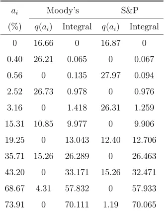
Table 5: Second order stochastic dominance of the distributions q(ai) ai Moody’s S&P (%) q(ai) Integral q(ai) Integral 0 16.66 0 16.87 0 0.40 26.21 0.065 0 0.067 0.56 0 0.135 27.97 0.094 2.52 26.73 0.978 0 0.976 3.16 0 1.418 26.31 1.259 15.31 10.85 9.977 0 9.906 19.25 0 13.043 12.40 12.706 35.71 15.26 26.289 0 26.463 43.20 0 33.171 15.26 32.471 68.67 4.31 57.832 0 57.933 73.91 0 70.111 1.19 70.065
where pi is the predicted probability of default, and θi = 1 in case of default
and θi = 0 in case of no default. It takes its optimum value of B = 0 when the
only predicted probabilities of default are 0 and 1, and when predictions are always correct (= perfect foresight). It takes its worst value of B = 1 when the only predicted probabilities of default are 0 and 1, and when always the opposite of what has been predicted occurs.
If we attach to each borrower the default probability from table 3, column 4 (Moody’s) and column 5 (S & P), we obtain
If we attach to each borrower the default probability from table 3, column 3, we obtain
BM = 0.0662, BS&P = 0.0689, (10)
and if we attach to each borrower the observed default rate of the class these borrower has been sorted into, we obtain
BM = 0.0660, BS&P = 0.0686. (11)
As small values of the Brier score are ”good”, Moody’s outperforms S&P ac-cording to this criterion. It also outperforms S&P acac-cording to the logarithmic score, defined as L= 1 n n X i=1 `n(|pi+θi−1|). (12)
The logarithmic score is always negative, with closeness to zero signalling a good performance. For our data set, it takes the following values if default probabilities from table 3 are used:
LM = −0.2185, LS&P =−0.2313 (column 4 and 5)
LM = −0.2116, LS&P =−0.2191 (column 3)
LM = −0.2109, LS&P =−0.2184 (column 1 and 2)
As large values of the logarithmic score are ”good”, Moody’s outperformS&P
also according to this criterion. They also outperform S&P according to the spherical score, defined as
S = 1 n n X i=1 |pi+θi−1| q p2 i + (1−pi)2 . (13)
This gives
SM = 0.9236, SS&P = 0.9173 (column 4 and 5)
SM = 0.9259, SS&P = 0.9226 (column 3)
SM = 0.9263, SS&P = 0.9229 (column 1 and 2)
As the spherical rule is always positive, with large values signalling superior performance, Moody’s wins here as well.
However, it is easy to find scores such that this ranking is reversed. This reversal is made possible by the noncomparability of Moody’s and S&P in terms of the empirical refinement ordering. It is well known that second order stochastic dominance of a distributionqB(a
i) by a distributionqA(ai) is equivalent to the
fact that X i g(ai)qA(ai)≥ X i g(ai)qB(ai) (14)
for all continuous convex functions g on the unit interval. On the other hand, it is also well known (see e.g. Winkler 1996; the basic theorem is due to Savage 1971) that, for well calibrated forecasters, all proper scoring rules
S(p1, . . . , pn;θ1, . . . , θn) depend on the pi and θi only via the aj’s and can
be written as S(p1, . . . , pn;θ1, . . . , θn) = K X j=1 g(aj)q(aj) (15)
with some strictly convex functiong. For the Brier score, for instance, we have
g(p) =p(1−p). (16)
If second order stochastic dominance fails, one can therefore always find two convex functions f and g (corresponding to two proper scoring rules Sf and
An example is the asymmetric version L∗ of the logarithmic score suggested
by Winkler (1994):
L∗ = [ln(|pi+θi−1|)−ln(|c+θi −1|)]/−ln(1−c) pi ≤c
[ln(|pi+θi−1|)−ln(|c+θi−1|)]/−ln(c) pi ≥c
. (17)
Setting c = 0.001 and equating observed default rates to predicted ones, we obtain values ofL∗,M = 0.2446 andL∗,S&P = 0.2456, so S&P is slightly better
now. For details, see Kr¨amer (2006).
5
Statistical Significance
Next we explicitly acknowledge the randomness in our data and briefly com-ment on the statistical significance of the differences in performance which we have found. For instance, the accuracy ratios derived from figure 1 are 0.833 for Moody’s (ARM) and 0.819 for S & P (ARS), so there is a slight but
in-significant advantage for Moody’s here. Engelmann et al. (2003) show that the statistic T = (ARM −ARS) 2 σ2 ARM +σ 2 ARS −2σARM,ARS (18) is asymptotically chi-squared with one degree of freedom. Approximating the variances σ2
ARS and σ
2
ARM and the covariance σARS,ARM of the respective
ac-curacy ratios ARS and ARM by bootstrapping produces a p-value of 0.087,
which does not indicate a systematic difference.
The asymptotic null distribution of theT-statistic (18) should be applied with caution, however. It assumes two independent simple random samples from the bivariate distributions [qM(a
j|1), qS(qj|1)] and [qM(aj|0), qS(aj|0)],
is met in the credit rating context. If we consider the 1927 ratings from the present paper as a random sample from a hypothetical universe of potential ratings, then the sample sizes n1 and n2 are not fixed but random and
per-fectly negatively correlated. And more importantly, a sample ofnobservations from the bivariate distribution r(θ, a) will in practice never be simple as the observed θ’s are known to be positively correlated in practice. As the observed values of θ anda for a given borrower are also highly correlated, this can then be shown to translate into correlation among draws from the conditional dis-tributions q(a|1) and q(a|0), which are therefore not a simple random sample. As H0 in our case is not rejected anyway, we do not investigate this issue any
further here.
The same argument applies even more forcefully when assessing the significance of the difference of other scalar measures of performance. For the Brier score, it is easily seen (see e.g. Redelmeier et al. 1991) that the statistic
Z = Pn i=1(θi−πi)(pSi −pMi ) qPn i=1πi(1−πi)(pSi −pMi )2 (19)
where πi = (pSi +pMi )/2, is asymptotically standard normal when population
Brier scores are identical. In our sample, Z takes the value 3.80, which at first sight is highly significant. However, as in the case of the Engelmann et al. T -statistic, its limiting null distribution obtains only for simple random samples, which in the rating context will almost never be observed in practice due to the positive correlation among the θ’s.
Diebold and Mariano (1995) show how to account for such correlations in a time series context. This approach might well translate into a cross-section environment, but we do not investigate this here any further since, for our data set, there do not seem to exist significant differences anyway.
6
Discussion
The basic message of our empirical application is that none of the two leading rating agencies seems to uniformly outperform the other (uniformly across measures of performance), confirming independent results from e.g. Ederington et al. (1987) or Moon and Stotsky (1993), who show that ratings by either agency convey information not contained in the rating of the other.
There are some shortcomings in our data, however. For instance, in order to obtain a reasonable data base, we had to collect all ratings as of Dec. 31, 1998 irrespective of the date the rating was produced or changed. This implies that the relative default frequencies from columns (1) - (3) in table 3 are for a horizon of slightly more than four years. For insurance, if a rating was issued on July 1 1998, the time horizon for default is four years and a half.
However, as ”no change” need not imply ”no assessment of creditworthyness”, and since both Moody’s and S&P are known for keeping a close track of their customers, the presumption is that the ratings observed in December 1998 closely mirror the then prevailing creditworthiness of the firms considered in our empirical example. Also, there are no large deviations in the age of the ratings between Moody’s and S&P, so this ”ragged edge” problem is unlikely to favor either of them.
Another question of course is whether or not our sample can be taken as typical for the performance of the agencies. It does not for instance cover a full business cycle but rather the end and apex of an extraordinary upswing and the beginning of a downturn in 2001 and 2002, were the majority of the defaults occurred. This might bias the absolute performance of both rating agencies. But since we are mainly concerned with relative performance, this possible sample bias is probably not as serious as it might seem at first sight.
References
Bluhm, C., Overbeck, L. and Wagner, L. (2003): An introduction to
credit risk modelling, Boca Raton (Chapman & Hall/CRC).
Brier, G.W. (1950): ”Verification of forecasts expressed in terms of proba-bility.” Monthly Weather Review 78, 1 – 3.
Carey, M. (2002): ”Some evidence on the consistency of banks’ internal credit ratings.” In: M. Ong (ed.) Credit ratings: Methodologies,
Ratio-nale and Default Risk, London (Risk Books).
Carey, M. and Hrycay, M. (2001): ”Parameterizing credit risk models with rating data.” Journal of Banking and Finance 25, 197 – 270. Crouhy, M., Galai, D. and Mark, R. (2001): ”Prototype risk rating
systems.” Journal of Banking and Finance 25, 47 – 95.
DeGroot, M. and Fienberg, S.E. (1983): ”The comparison and evalua-tion of probability forecasters.” The Statistican 32, 12 – 22.
Diebold, F.X. and Mariano, R.S. (1995): ”Comparing Predictive Accu-racy.” Journal of Business and Economic Statistics 13, 99 – 118.
Ederington, L.H. (1986): ”Why split ratings occur.” Financial Manage-ment 16, 47 – 47.
Ederington, L.H., Yawitz, J.B. and Roberts. B.E. (1987): ”The in-formational content of bond ratings.” Journal of Financial Research 10, 211 – 226.
Engelmann, B., Hayden, E. and Tasche, D. (2003): ”Testing rating accuracy.” Risk 16, 82 – 86.
Falkenstein, E. (2000): ”Validating commercial risk grade mappings: why and how.” Journal of Lending and Credit Risk Management, Feb., 26 – 33.
Kr¨amer, W. (2003): ”Die Bewertung und der Vergleich von Kreditausfall-prognosen.” Kredit und Kapital 36, 325-340.
Kr¨amer, W. (2005): ”On the ordering of probability forecasts.” Sankhya
67, 662 – 669.
Kr¨amer, W. (2006): ”Evaluating probability forecasts in terms of refine-ment and strictly proper scoring rules.” Journal of Forecasting25, 223 – 226.
Moon, C.G. and Stotsky, J.G. (1993): ”Testing the difference between the determinante of Moody’s and Standard & Poor’s ratings: An appli-cation of smooth simulated Maximum Likelihood estimation.” Journal
of Applied Econometrics 8, 51 – 69.
Redelmeier, D.A., Block, D.A. and Hickam, D.H. (1991): ”Assessing predictive accuracy: How to compare Brier scores.” Journal of Clinical
Epidemiology 44, 1141 – 1146.
Savage, L.J. (1971): ”Elicitation of personal probabilities and expecta-tions.” Journal of the American Statistical Association 66, 783 – 801. Sobehart, J. and Keenan, S. (2001) : ”Measuring default risk
accura-tely”, Risk, 31 – 33.
Vardemann, S. and Meeden, G. (1983): ”Calibration, sufficiency and domination: Considerations for Bayesian probability assessors.” Journal
of the American Statistical Association 78, 808 – 816.
Winkler, R.L. (1994): ”Evaluating probabilities: Asymmetric scoring rules.” Management Science40, 1395 – 1405.
Winkler, R.L. (1996): ”Scoring rules and the evaluation of probabilities.”
CESifo Working Paper Series
for full list see Twww.cesifo-group.org/wpT(address: Poschingerstr. 5, 81679 Munich, Germany, [email protected])
___________________________________________________________________________ 2140 Lorenzo Cappellari, Paolo Ghinetti and Gilberto Turati, On Time and Money
Donations, November 2007
2141 Roel Beetsma and Heikki Oksanen, Pension Systems, Ageing and the Stability and Growth Pact, November 2007
2142 Hikaru Ogawa and David E. Wildasin, Think Locally, Act Locally: Spillovers, Spillbacks, and Efficient Decentralized Policymaking, November 2007
2143 Alessandro Cigno, A Theoretical Analysis of the Effects of Legislation on Marriage, Fertility, Domestic Division of Labour, and the Education of Children, November 2007 2144 Kai A. Konrad, Mobile Tax Base as a Global Common, November 2007
2145 Ola Kvaløy and Trond E. Olsen, The Rise of Individual Performance Pay, November 2007
2146 Guglielmo Maria Caporale, Yannis Georgellis, Nicholas Tsitsianis and Ya Ping Yin, Income and Happiness across Europe: Do Reference Values Matter?, November 2007 2147 Dan Anderberg, Tax Credits, Income Support and Partnership Decisions, November
2007
2148 Andreas Irmen and Rainer Klump, Factor Substitution, Income Distribution, and Growth in a Generalized Neoclassical Model, November 2007
2149 Lorenz Blume, Jens Müller and Stefan Voigt, The Economic Effects of Direct Democracy – A First Global Assessment, November 2007
2150 Axel Dreher, Pierre-Guillaume Méon and Friedrich Schneider, The Devil is in the Shadow – Do Institutions Affect Income and Productivity or only Official Income and Official Productivity?, November 2007
2151 Valentina Bosetti, Carlo Carraro, Emanuele Massetti and Massimo Tavoni, International Energy R&D Spillovers and the Economics of Greenhouse Gas Atmospheric Stabilization, November 2007
2152 Balázs Égert and Dubravko Mihaljek, Determinants of House Prices in Central and Eastern Europe, November 2007
2153 Christa Hainz and Hendrik Hakenes, The Politician and his Banker, November 2007 2154 Josef Falkinger, Distribution and Use of Knowledge under the “Laws of the Web”,
2155 Thorvaldur Gylfason and Eduard Hochreiter, Growing Apart? A Tale of Two Republics: Estonia and Georgia, December 2007
2156 Morris A. Davis and François Ortalo-Magné, Household Expenditures, Wages, Rents, December 2007
2157 Andreas Haufler and Christian Schulte, Merger Policy and Tax Competition, December 2007
2158 Marko Köthenbürger and Panu Poutvaara, Rent Taxation and its Intertemporal Welfare Effects in a Small Open Economy, December 2007
2159 Betsey Stevenson, Title IX and the Evolution of High School Sports, December 2007 2160 Stergios Skaperdas and Samarth Vaidya, Persuasion as a Contest, December 2007 2161 Morten Bennedsen and Christian Schultz, Arm’s Length Provision of Public Services,
December 2007
2162 Bas Jacobs, Optimal Redistributive Tax and Education Policies in General Equilibrium, December 2007
2163 Christian Jaag, Christian Keuschnigg and Mirela Keuschnigg, Pension Reform, Retirement and Life-Cycle Unemployment, December 2007
2164 Dieter M. Urban, Terms of Trade, Catch-up, and Home Market Effect: The Example of Japan, December 2007
2165 Marcelo Resende and Rodrigo M. Zeidan, Lionel Robbins: A Methodological Reappraisal, December 2007
2166 Samuel Bentolila, Juan J. Dolado and Juan F. Jimeno, Does Immigration Affect the Phillips Curve? Some Evidence for Spain, December 2007
2167 Rainald Borck, Federalism, Fertility and Growth, December 2007
2168 Erkki Koskela and Jan König, Strategic Outsourcing, Profit Sharing and Equilibrium Unemployment, December 2007
2169 Egil Matsen and Øystein Thøgersen, Habit Formation, Strategic Extremism and Debt Policy, December 2007
2170 Torben M. Andersen and Allan Sørensen, Product Market Integration and Income Taxation: Distortions and Gains from Trade, December 2007
2171 J. Atsu Amegashie, American Idol: Should it be a Singing Contest or a Popularity Contest?, December 2007
2173 Ben Greiner, Axel Ockenfels and Peter Werner, The Dynamic Interplay of Inequality and Trust – An Experimental Study, December 2007
2174 Michael Melvin and Magali Valero, The Dark Side of International Cross-Listing: Effects on Rival Firms at Home, December 2007
2175 Gebhard Flaig and Horst Rottmann, Labour Market Institutions and the Employment Intensity of Output Growth. An International Comparison, December 2007
2176 Alexander Chudik and M. Hashem Pesaran, Infinite Dimensional VARs and Factor Models, December 2007
2177 Christoph Moser and Axel Dreher, Do Markets Care about Central Bank Governor Changes? Evidence from Emerging Markets, December 2007
2178 Alessandra Sgobbi and Carlo Carraro, A Stochastic Multiple Players Multi-Issues Bargaining Model for the Piave River Basin, December 2007
2179 Christa Hainz, Creditor Passivity: The Effects of Bank Competition and Institutions on the Strategic Use of Bankruptcy Filings, December 2007
2180 Emilia Del Bono, Andrea Weber and Rudolf Winter-Ebmer, Clash of Career and Family: Fertility Decisions after Job Displacement, January 2008
2181 Harald Badinger and Peter Egger, Intra- and Inter-Industry Productivity Spillovers in OECD Manufacturing: A Spatial Econometric Perspective, January 2008
2182 María del Carmen Boado-Penas, Salvador Valdés-Prieto and Carlos Vidal-Meliá, the Actuarial Balance Sheet for Pay-As-You-Go Finance: Solvency Indicators for Spain and Sweden, January 2008
2183 Assar Lindbeck, Economic-Social Interaction in China, January 2008
2184 Pierre Dubois, Bruno Jullien and Thierry Magnac, Formal and Informal Risk Sharing in LDCs: Theory and Empirical Evidence, January 2008
2185 Roel M. W. J. Beetsma, Ward E. Romp and Siert J. Vos, Intergenerational Risk Sharing, Pensions and Endogenous Labor Supply in General Equilibrium, January 2008
2186 Lans Bovenberg and Coen Teulings, Rhineland Exit?, January 2008
2187 Wolfgang Leininger and Axel Ockenfels, The Penalty-Duel and Institutional Design: Is there a Neeskens-Effect?, January 2008
2188 Sándor Csengődi and Dieter M. Urban, Foreign Takeovers and Wage Dispersion in Hungary, January 2008
2189 Joerg Baten and Andreas Böhm, Trends of Children’s Height and Parental Unemployment: A Large-Scale Anthropometric Study on Eastern Germany, 1994 –
2190 Chris van Klaveren, Bernard van Praag and Henriette Maassen van den Brink, A Public Good Version of the Collective Household Model: An Empirical Approach with an Application to British Household Data, January 2008
2191 Harry Garretsen and Jolanda Peeters, FDI and the Relevance of Spatial Linkages: Do third Country Effects Matter for Dutch FDI?, January 2008
2192 Jan Bouckaert, Hans Degryse and Theon van Dijk, Price Discrimination Bans on Dominant Firms, January 2008
2193 M. Hashem Pesaran, L. Vanessa Smith and Takashi Yamagata, Panel Unit Root Tests in the Presence of a Multifactor Error Structure, January 2008
2194 Tomer Blumkin, Bradley J. Ruffle and Yosef Ganun, Are Income and Consumption Taxes ever really Equivalent? Evidence from a Real-Effort Experiment with Real Goods, January 2008
2195 Mika Widgrén, The Impact of Council’s Internal Decision-Making Rules on the Future EU, January 2008
2196 Antonis Adam, Margarita Katsimi and Thomas Moutos, Inequality and the Import Demand Function, January 2008
2197 Helmut Seitz, Democratic Participation and the Size of Regions: An Empirical Study Using Data on German Counties, January 2008
2198 Theresa Fahrenberger and Hans Gersbach, Minority Voting and Long-term Decisions, January 2008
2199 Chiara Dalle Nogare and Roberto Ricciuti, Term Limits: Do they really Affect Fiscal Policy Choices?, January 2008
2200 Andreas Bühn and Friedrich Schneider, MIMIC Models, Cointegration and Error Correction: An Application to the French Shadow Economy, January 2008
2201 Seppo Kari, Hanna Karikallio and Jukka Pirttilä, Anticipating Tax Change: Evidence from the Finnish Corporate Income Tax Reform of 2005, January 2008
2202 Walter Krämer and André Güttler, On Comparing the Accuracy of Default Predictions in the Rating Industry, January 2008