THE EFFECTS OF MICRO-VORTEX GENERATORS ON NORMAL SHOCK WAVE/BOUNDARY LAYER INTERACTIONS
BY
THOMAS G. HERGES
DISSERTATION
Submitted in partial fulfillment of the requirements
for the degree of Doctor of Philosophy in Aerospace Engineering in the Graduate College of the
University of Illinois at Urbana-Champaign, 2013
Urbana, Illinois
Doctoral Committee:
Professor Gregory S. Elliott, Chair and Co-Director of Research Professor J. Craig Dutton, Co-Chair and Co-Director of Research Professor Michael B. Bragg
ii
ABSTRACT
Shock wave/boundary-layer interactions (SWBLIs) are complex flow phenomena that are important in the design and performance of internal supersonic and transonic flow fields such as engine inlets. This investigation was undertaken to study the effects of passive flow control devices on normal shock wave/boundary layer interactions in an effort to gain insight into the physics that govern these complex interactions. The work concentrates on analyzing the effects of vortex generators (VGs) as a flow control method by contributing a greater understanding of the flowfield generated by these devices and characterizing their effects on the SWBLI. The vortex generators are utilized with the goal of improving boundary layer health (i.e., reducing/increasing the boundary-layer incompressible shape factor/skin friction coefficient) through a SWBLI, increasing pressure recovery, and reducing flow distortion at the aerodynamic interface plane while adding minimal drag to the system. The investigation encompasses experiments in both small-scale and large-scale inlet testing, allowing multiple test beds for improving the characterization and understanding of vortex generators.
Small-scale facility experiments implemented instantaneous schlieren photography, surface oil-flow visualization, pressure-sensitive paint, and particle image velocimetry to characterize the effects of an array of microramps on a normal shock wave/boundary-layer interaction. These diagnostics measured the time-averaged and instantaneous flow organization in the vicinity of the microramps and SWBLI. The results reveal that a microramp produces a complex vortex structure in its wake with two primary counter-rotating vortices surrounded by a train of Kelvin- Helmholtz (K-H) vortices. A streamwise velocity deficit is observed in the region of the primary vortices in addition to an induced upwash/downwash which persists through the normal shock with reduced strength. The microramp flow control also increased the spanwise-averaged skin-friction coefficient and reduced the spanwise-averaged incompressible shape factor, thereby improving the health of the boundary layer. The velocity in the near-wall region appears to be the best indicator of microramp effectiveness at controlling SWBLIs.
Continued analysis of additional micro-vortex generator designs in the small-scale facility revealed reduced separation within a subsonic diffuser downstream of the normal shock wave/boundary layer interaction. The resulting attached flow within the diffuser from the micro-vortex generator control devices reduces shock wave position and pressure RMS fluctuations within the diffuser along with increased pressure recovery through the shock and at the entrance of the diffuser. The largest effect was observed by the micro-vortex generators that produce the strongest streamwise vortices. High-speed pressure measurements also indicated that the vortex generators shift the energy of the pressure fluctuations to higher frequencies.
iii
Implementation of micro-vortex generators into a large-scale, supersonic, axisymmetric, relaxed-compression inlet have been investigated with the use of a unique and novel flow-visualization measurement system designed and successfully used for the analysis of both upstream micro-VGs (MVGs) and downstream VGs utilizing surface oil-flow visualization and pressure-sensitive paint measurements. The inlet centerbody and downstream diffuser vortex-generator regions were imaged during wind-tunnel testing internally through the inlet cowl with the diagnostic system attached to the cowl. Surface-flow visualization revealed separated regions along the inlet centerbody for large mass-flow rates without vortex generators. Upstream vortex generators did reduce separation in the subsonic diffuser, and a unique perspective of the flowfield produced by the downstream vortex generators was obtained. In addition, pressure distributions on the inlet centerbody and vortex generators were measured with pressure-sensitive paint.
At low mass-flow ratios the onset of buzz occurs in the large-scale low-boom inlet. Inlet buzz and how it is affected by vortex generators was characterized using shock tracking through high-speed schlieren imaging and pressure fluctuation measurements. The analysis revealed a dominant low frequency oscillation at 21.0 Hz for the single-stream inlet, corresponding with the duration of one buzz cycle. Pressure oscillations prior to the onset of buzz were not detected, leaving the location where the shock wave triggers large separation on the compression spike as the best indicator for the onset of buzz. The driving mechanism for a buzz cycle has been confirmed as the rate of depressurization and repressurization of the inlet as the buzz cycle fluctuates between an effectively unstarted (blocked) inlet and supercritical operation (choked flow), respectively. High-frequency shock position oscillations/pulsations (spike buzz) were also observed throughout portions of the inlet buzz cycle. The primary effect of the VGs was to trigger buzz at a higher mass-flow ratio.
iv
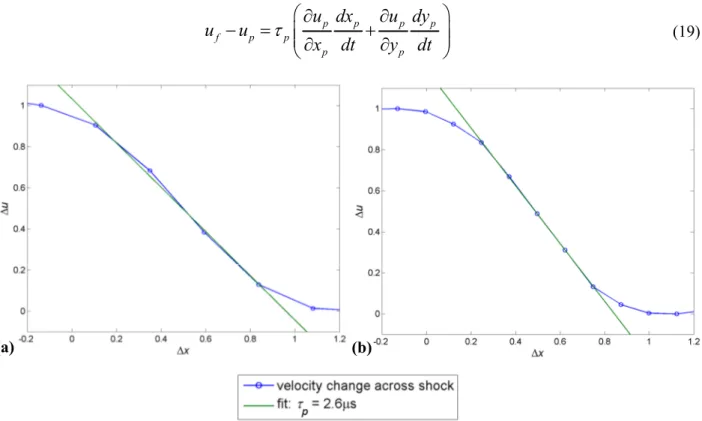
ACKNOWLEDGMENTS
Most importantly this work is dedicated to my loving parents, Geno and Patty, and sister, Amy. You all have always been amazingly encouraging and unconditionally supportive in all of my endeavors. Thank you for inspiring me to work hard and fueling my passion for learning and wonderment. I have truly loved my time at the University of Illinois, forever having a place in my heart as I bleed Orange and Blue. I am thankful that you all have been able to share in my time and love of this place, allowing Amy and me to become close siblings.
I would like to thank my doctoral research advisors, Professor Craig Dutton and Professor Greg Elliott for their support, encouragement, and insight through the learning process of being a researcher as we all work to discover and understand more. Thank you for the patience and guidance as I continue to learn; I know that my learning has not always stayed on the most direct path to completing this document. Thank you also to the remaining members of my dissertation committee, Professor Michael Bragg and Professor Kenneth Christensen for their expertise and assistance in reviewing and helping to improve this work.
Thank you to my friends and colleagues, Todd Reedy, Bill Flaherty, Ryan Fontaine, Albert Lee, Chris Cirone, Andrew Knisely, Brad DeBlauw, Andy Swantek, Wilbur Chang, Nachiket Kale, Brad Sanders, Becca Ostman, Ruben Hortensius, Erik Kroeker, Eli Lazar, Jason Hale, and Michael Rybalko (and to many other personal friends that I haven’t named). I have enjoyed this journey with you and I am better for having known you. Additional acknowledgements are extended to the undergraduate research assistants, Piotr Szponder and Robyn McDonald, for their time and efforts.
Thank you to Greg Milner, Yeol Lee, Jim Crafton, Stefanie Hirt, Professor Eric Loth, Tim Conners, Tom Wayman and Rod Chima for their technical assistance on this wonderful project that I am happy to have been a part of. Thank you to the 8’x6’ supersonic wind tunnel team at NASA Glenn Research Center for their work on tunnel program management, tunnel integration, and test execution in addition to Tri Models Inc. for completing the final mechanical design, construction, and instrumentation of the LSLB inlet model. Finally, thank you to Gulfstream, Rolls Royce, and the NASA Fundamental Aeronautics Program, Supersonics Project for the funding for this work.
v
TABLE OF CONTENTS
LIST OF ABBREVIATIONS ... vii
LIST OF SYMBOLS ... viii
CHAPTER 1 : INTRODUCTION ... 1
1.1 Supersonic Inlet Shock Wave/Boundary Layer Interaction ... 2
1.2 Flow Control Methods ... 4
1.3 Motivation and Objectives ... 5
CHAPTER 2 : MICRORAMP BOUNDARY LAYER CHARACTERIZATION ... 7
2.1 Introduction and Background ... 7
2.2 Experimental Arrangement ... 11
2.3 Schlieren Measurements ... 32
2.4 Surface Oil Flow Results ... 35
2.5 Pressure-Sensitive Paint Measurements ... 38
2.6 Particle Image Velocimetry ... 41
2.7 Summary and Conclusions ... 61
CHAPTER 3 : FLOW CONTROL SHOCK STABILITY ... 63
3.1 Introduction and Background ... 63
3.2 Experimental Arrangement ... 66
3.3 Schlieren Imaging ... 72
3.4 Surface Oil-Flow Visualization Results ... 78
3.5 Pressure Fluctuation Measurements ... 81
3.6 Summary and Conclusions ... 90
CHAPTER 4 : LARGE-SCALE LOW-BOOM INLET TEST ... 91
4.1 Introduction and Background ... 91
4.2 Experimental Arrangement ... 93
4.3 Surface Flow Results ... 100
4.4 Pressure-Sensitive Paint Measurements ... 110
4.5 Summary and Conclusions ... 125
CHAPTER 5 : LARGE-SCALE LOW-BOOM INLET BUZZ ... 127
5.1 Introduction and Background ... 127
5.2 Inlet Dynamic Instrumentation and Operation ... 133
5.3 Inlet Buzz Characterization... 136
vi
5.5 Additional Shock Wave and Pressure Fluctuation Comparisons ... 150
5.6 Summary and Conclusions ... 154
CHAPTER 6 : CONCLUSIONS AND RECOMMENDATIONS ... 156
6.1 Research Summary and Conclusions ... 156
6.2 Suggestions for Future Work ... 159
REFERENCES ... 161
APPENDIX A: SHEAR STRESS MEASUREMENTS ... 171
A.1 Introduction and Background ... 171
A.2 Experimental Arrangement ... 171
A.3 Surface Stress Sensitive Film Measurements ... 179
A.4 Summary and Conclusions ... 188
APPENDIX B: CAMERA HOUSING WATER COOLING ... 189
vii
LIST OF ABBREVIATIONS
AOA = angle of attackAIP = aerodynamic interface plane CCD = charge-coupled device CFD = computational fluid dynamics
CMOS = complementary metal-oxide-semiconductor D0 = no downstream control (LSLB inlet) D1 = large downstream vane (upwash) D2 = large downstream vane (downwash) D3 = large downstream plow
D4 = large downstream ramp
D5 = small downstream vane (downwash) D6 = small downstream ramp
DEHS = diethylhexyl sebacate DES = detached eddy simulation DNS = direct-numerical simulation FEA = finite element analysis GRC = Glenn Research Center
ILES = implicit large eddy simulations ISSI = Innovative Scientific Solutions Inc. K-H = Kelvin-Helmholtz
LED = light emitting diode LES = large-eddy simulation LSLB = large-scale low-boom MFR = mass-flow ratio MVG = micro-vortex generator
Nd: YAG = neodymium-doped yttrium aluminum garnet PDF = probability density function
PIV = particle image velocimetry PTV = particle tracking velocimetry PSD = power spectral density PSP = pressure-sensitive paint
RANS = Reynolds-averaged Navier-Stokes RMS = root mean square
RSM = response surface method S3F = Surface Stress Sensitive Film SBVG = sub-boundary layer vortex generator SWBLI = shock wave/boundary layer interaction U0 = no upstream control (LSLB inlet) U1 = large upstream microramp U2 = small upstream microramp U3 = large upstream split-ramp U4 = small upstream split-ramp VG = vortex generator
viii
LIST OF SYMBOLS
A = area
A(T) = Stern-Volmer coefficient (Equation (11)) Ap = microramp angle of incidence
a = constant used in modified wall-wake profile ap = particle acceleration, m/s
2
B(T) = Stern-Volmer coefficient (Equation (11)) C = constant in Law of the Wall, usually equals 5.2 Cf = skin friction coefficient, τw/[(1/2) ρeue
2
] c = vortex generator chord length, mm cp = specific heat, J/(kg K)
D = cavity depth, mm
d = distance from camera lens to calibration scale, mm dp = particle diameter, µm
f = frequency, Hz
G(f) = power spectral density
H = incompressible boundary-layer shape factor, δ*/θ Htr = transformed form factor
h = vortex generator height, mm I = image intensity
i = horizontal pixel location j = vertical pixel location
K = Von Karman’s constant, usually equals 0.41 Kn = Knudsen number (Equation (17))
k = thermal conductivity, W/(m K), or Rossiter convective velocity, 0.57 L = characteristic length, mm, or length of scale used for calibration, pixels l = length of scale used for calibration, mm
M = Mach number
M∞ = freestream Mach number
m = Rossiter mode of oscillation N = number of samples
n = acoustic frequency mode Pr = Prandtl number (µcp/k)
p = static pressure, kPa po = stagnation pressure, kPa
p∞ = freestream static pressure, kPa
R = coefficient of determination Re∞ = unit Reynolds number
Reθ = Reynolds number based on incompressible momentum thickness
Reδ2 = Reynolds number based on incompressible momentum thickness and density at wall
r = recovery factor for turbulent boundary layer, r = Pr1/3 S = sensitivity coefficient
St = Stern-Volmer constant (Equation (12))
StL = Strouhal number (Equation (24))
s = spanwise vortex generator spacing, mm T = temperature, K
t = time, s
U∞ = mean freestream velocity in streamwise direction, m/s
ix ũ = velocity in streamwise direction, pixel/s uτ = wall-friction velocity, (τw/ρw)
1/2 , m/s
u+ = mean velocity in streamwise direction in inner-wall coordinates, u/uτ
uʹ = turbulence intensity in streamwise direction, m/s uʹvʹ = Reynolds shear stress, m2/s2
v = velocity in wall-normal direction, m/s
vʹ = turbulence intensity in wall-normal direction, m/s w = uncertainty value, or velocity in spanwise direction, m/s wʹ = turbulence intensity in spanwise direction, m/s
Xd = distance between diffuser shoulder and microramp array, mm Xs = distance between normal shock and microramp array, mm x = streamwise coordinate, mm
y = wall-normal coordinate, mm
y+ = wall-normal coordinate in inner-wall coordinates, yuτ/νw
z = spanwise coordinate, mm zc = confidence coefficient
α = angle of attack, degrees, or Rossiter constant, 0.062(L/D) γ = ratio of specific heats
∆ = change in property
δ = boundary-layer thickness, mm
δ* = boundary-layer incompressible displacement thickness, mm ε = mass-flow ratio, A∞/Ac
θ = boundary-layer incompressible momentum thickness, mm η = y/δ, inlet pressure recovery, po,AIP/po,∞
λ = wavelength, mm, or distance from camera lens to calibration scale, mm µ = absolute viscosity, kg/(s m)
ν = kinematic viscosity, m2/s ξp = particle relaxation length, µm
Π = wake parameter ρ = density, kg/m3
σ = standard deviation, or parameter used in modified wall-wake profile τ = shear stress, kPa
τp = particle relaxation time, µs
φ = pressure-sensitive paint uncertainty parameter (Equation (13))
Subscripts
a = acoustic
c = inlet capture d = diffuser
ds = dual-stream inlet
e = conditions at the edge of the boundary layer, inlet exit w = conditions at wall
p = particle
s = shock
ss = single-stream inlet
∞ = incoming freestream condition o = total or stagnation condition
1
Chapter 1: Introduction
Over many years extensive research has been conducted on the subject of shock wave/boundary layer interactions (SWBLIs) due to the important influence shock waves have, for example, on supersonic inlets and transonic aircraft. SWBLIs are a complex flow phenomenon with many facets and continuing research in order to provide a deeper understanding. SWBLIs are especially important for the design and performance of internal supersonic and transonic flow fields such as engine intakes where such interactions can cause unsteady separation of the boundary layer and fluctuating pressure loads [1-3]. This emphasizes the importance of controlling the SWBLIs in supersonic inlets, where the SWBLI exerts a dominant influence over the subsonic flowfield downstream of the shock [4].
An inlet’s function in the propulsion system is to capture and decelerate flow to a Mach number and pressure suitable for the engine fan face, with minimal losses and distortions, while maintaining minimal external drag [5]. Often with such designs, supersonic inlets contain an additional subsonic diffuser following the initial compression of a shock wave system created with a supersonic diffuser. The adverse pressure gradient produced by shock waves can create boundary layer separation if the SWBLIs are strong enough. In a supersonic inlet this can lead to downstream spatial distortions at the engine compressor blades due to the propagation of separated flow in the diffuser. Inlet unstart can even occur as a result of excess boundary-layer thickening [6].
Early work on supersonic inlets dictated using a series of oblique shock waves to decelerate the flow to a low local Mach number of approximately 1.33 upstream of the terminating shock in order to generate an incipiently separated flow [7]. In the past, detailed examination of the physics involving flow control methods in large-scale inlet tests was often unrealistic due to the complexity and cost of these tests. Historically, supersonic inlet tests focused on analyzing the inlet performance directly with pressure tap rakes at the aerodynamic interface plane (AIP) and mass-flow ratio (MFR) measurements without evaluating the fundamental flow physics in the throat region near the SWBLI [8]. Boundary-layer suction, or bleed, became the inlet flow control technique of choice due its ability to suppress shock-induced separation and maintain shock position, reducing shock oscillations and flow unsteadiness [9]. Although effective, the removal of the low-momentum fluid in the near-wall region reduces the mass flow to the engine. Thus, bleed can necessitate added weight and volume to the propulsion system design, as well as mechanical complexity. It is these limitations that have led to alternative SWBLI control research [10, 11].
Many fundamental investigations into SWBLIs have been conducted, with numerous thorough reviews of these works offering insight into the physics of SWBLIs [1, 12-14]. Recent fundamental
2
studies have investigated the use of sub-boundary layer vortex generators (SBVGs) in order to replace, or augment, bleed as a method of reducing SWBLI separation, improving boundary layer health in supersonic inlets, and reducing shock unsteadiness [6, 10, 11, 15-21]. Improved boundary-layer health is characterized by a reduced incompressible shape factor, H, and/or an increased skin-friction coefficient, Cf. By reducing the need for conventional bleed systems, future supersonic inlets can be designed with
simpler geometries and optimal aerodynamic properties with less drag and weight [22-24]. Therefore, experimental research and further fundamental understanding of SWBLIs and their control are of substantial importance along with a greater comprehension of how these results translate into better supersonic inlet performance.
1.1 Supersonic Inlet Shock Wave/Boundary Layer Interaction
For an ideal shock wave, the pressure on the surface would increase discontinuously through the shock wave. In the presence of a boundary layer this abrupt pressure rise cannot occur [12]. The viscous flow adjacent to the wall in the inner part of the boundary layer has a subsonic velocity and is unable to undergo a discontinuous change in pressure. Because of this, the overall pressure rise is partially transmitted upstream through the subsonic part of the boundary layer resulting in the divergence of the streamlines in the subsonic region. This creates compression waves in the outer, supersonic region of the flow. Consequently, this aspect is the fundamental element in the nature of a SWBLI, where the shock modifies the boundary layer, which in turn affects the shock structure. The details and nature of the interaction depend on a wide range of flow parameters such as the boundary layer Reynolds number, shape factor, and pressure rise [3].
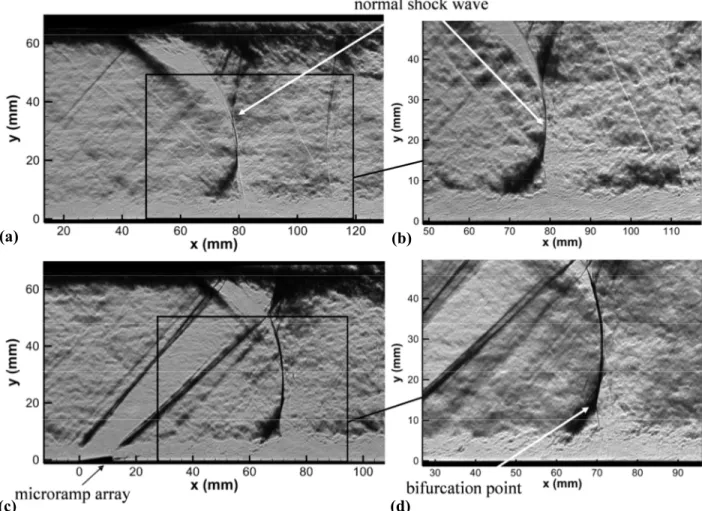
At low Mach numbers, the pressure rise across the shock is too small to cause the boundary layer to separate [12, 25]. As shown in Fig. 1a, the subsonic portion of the unseparated boundary layer thickens upstream of the shock, causing compression waves to emanate from the sonic line which eventually coalesce forming a foot for the outer shock. The wall static pressure increases in a continuous fashion, while the static pressure in the core flow increases discontinuously, reflecting the mixed subsonic/supersonic nature of the interaction [25]. Such normal shock interactions, where the downstream flow is totally or partially subsonic, are of special interest because of the possibility that downstream disturbances can influence the shock and initiate an interactive process at the origin of large-scale unsteadiness involving the whole flow, as in transonic buffeting or air-intake buzz [14].
Across a strong shock wave the inertia forces in the subsonic layer near the wall are not strong enough to negotiate the increased pressure rise causing the boundary layer to separate at the foot of the shock (Fig. 1b). This will thereby increase the complexity of the interaction. Weak oblique compression waves coalesce to form a weak oblique shock, or leading shock, which eventually intersects the strong,
3
nearly normal shock in the outer supersonic flow at the bifurcation, or triple, point. At this point a second weak oblique shock, or trailing shock, is generated which propagates back toward the wall. This structure is referred to as a lambda shock with the triple point being approximately 4-5 boundary-layer heights above the surface [25-29]. In these interactions the surface pressure rises modestly through the separated region, and the flow reattaches by a process of strong interaction between the boundary layer and freestream.
Figure 1: Shock wave/boundary layer interaction schematics: (a) unseparated normal shock [25], and (b) separated normal shock (derived from [27]).
The dynamical behavior of the interaction is known to exhibit a wide range of spatial and temporal scales [2, 30]. In order to accurately describe these interactions and fully understand their unsteadiness, experimental studies, numerical large-eddy simulation (LES), and direct-numerical simulation (DNS) methods are required. The nature of the interaction unsteadiness involves both low and high frequency aspects [3]. These local features consist of small-scale shock oscillations as well as unsteady separation and reattachment processes accompanied with global flow oscillations [31]. This includes large-scale low-frequency motion of the shock wave system and separated region that is orders of magnitude lower in frequency than the incoming boundary layer frequency. Much work has been conducted trying to correlate the high-frequency perturbations of the incoming boundary layer and freestream with the low-frequency oscillations of shock waves. Evidence has shown a correlation between upstream boundary layer velocity fluctuations and oscillations in the shock foot position occurring at the separation point [13, 14, 30, 32, 33]. Other studies have seen a greater correlation between shock oscillations and downstream large-scale fluctuations created from the flapping of the mixing layer surrounding the expanding and contracting separation bubble of the SWBLI [13, 14, 31, 34-37]. Shock wave oscillations have also been found to be triggered from downstream pressure perturbations and wind tunnel or inlet acoustical effects [38, 39]. normal shock M< 1 vortex sheet supersonic tongue bubble y/δ∞ δ∞ x/δ∞ boundary layer M≈ 1.4 rear shock leading shock : supersonic : separation unshaded: subsonic (a) (b)
4
1.2 Flow Control Methods
As previously discussed, passive SWBLI control methods may offer a lower weight, cost, and drag solution for supersonic inlet design [8, 40]. Thus, research has been conducted on various passive shock wave/boundary layer interaction control devices. These control methods have included micro-vortex generators, such as microramps [6, 17, 18], open cavities [41], streamwise slots [42], 3D bumps [43], mesoflaps [44], and porous plates over open cavities [45]. The criterion for flow separation corresponds to a velocity gradient of zero at the wall, or zero wall friction. These separation control techniques can be classified into the following four general approaches to mitigating a near-wall velocity gradient of zero: decrease the imposed adverse pressure gradient, impose a wall slip layer, remove the low-momentum near-wall flow, or add momentum to the near-wall flow [40].
The most popular flow control method to emerge from these various studies, as well as the control method primarily presented currently (micro-vortex generators), sweeps high momentum fluid from the outer boundary layer into the near-wall region, thus helping to energize the boundary layer and reducing the likelihood of separation [6]. Numerous studies have investigated the use of sub-boundary layer vortex generators (SBVGs) as a method of reducing SWBLI separation and improving boundary layer health in supersonic inlets [5, 6, 10, 11, 15-18, 20, 21, 46]. These sub-boundary layer, micro-, or low-profile vortex generators are similar to traditional vortex generators, but have heights less than the boundary layer thickness [10]. Micro-vortex generators (MVGs) are positioned upstream of the SWBLI, and have been shown to eliminate or reduce separation by inducing vorticity into the near-wall region. MVGs generate streamwise vortices that entrain high-momentum flow to energize the low-momentum portion of the boundary layer. It is believed that their smaller heights can reduce parasitic drag while maintaining similar levels of entrainment observed with traditional vortex generators [6, 10, 11, 15, 16]. This concept was proven with force balance measurements demonstrating the reduced drag of micro-vortex generator devices compared with traditional vanes [40]. Many designs of MVGs have been studied. These designs include vanes [11, 18, 19], forward-facing wedges or ramps [6, 17-19], backward-facing wedges or plows [11, 47], robust vanes [20], ramped vanes and split-ramps [19, 21, 48]. An additional row of staggered microramps has been shown to further reduce separation of an SWBLI [2].
Early pioneering studies involving ramp-type, low-profile vortex generators for normal shock wave/boundary-layer interaction control revealed that the VGs significantly suppressed the shock-induced separation bubble. Reduced boundary-layer losses with improved boundary-layer characteristics and static pressure recovery downstream of the shock were also observed [16, 49]. Unfortunately, the suppression of the separation bubble resulted in an increase in total pressure loss through the shock system. Nevertheless, McCormick [16] recommended the application of micro-vortex generators in
5
supersonic diffusers citing that the increased pressure recovery should more than make up for the increased shock loss. Early computational analysis confirmed the alleviation of shock-induced separation using a 3D multiblock, multizone, time-dependent Euler/Navier-Stokes solution algorithm [26]. The computational results indicated that the best placement of the VGs is at a sufficient distance upstream of the shock to ensure ample time and distance, for the generated streamwise vortices to energize the low-momentum boundary-layer flow near the surface.
Most recently, the investigation of these control devices on SWBLIs was extended into the testing of the Gulfstream large-scale low-boom (LSLB) inlet with both numerical and experimental methods. The investigation included analyzing the effects of the vortex generators near the SWBLI as well as the effects on the inlet aerodynamic performance. Reynolds-averaged Navier-Stokes (RANS) methods provided numerical simulations investigating the effects of MVGs on the separation generated by the normal shock wave and on the radial distortion at the AIP it creates [50]. It was discovered that micro-vortex generators placed upstream of the normal shock wave did significantly reduce separation downstream of the terminating normal shock near the geometric throat of the inlet, but had no noticeable effect at the AIP. The vortices produced by the upstream MVGs dissipated before reaching the AIP. Because of this, further RANS simulations showed that traditional vanes and ramps placed in the diffuser of the LSLB inlet, with a height on the order of the boundary layer thickness, reduced radial distortion at the AIP [50, 51]. The experimentally measured effect of VGs in the LSLB inlet will be described in the present work. Investigations such as the LSLB inlet experiment provide a means of coupling the observed effect of passive flow control devices between fundamental wind tunnel work and supersonic inlet applications.
1.3 Motivation and Objectives
The objective of this dissertation is to study the effects of passive flow control devices on normal shock wave/boundary layer interactions in an effort to gain insight into the physics that govern these complex interactions. The work will concentrate on analyzing the effects of vortex generators by contributing a greater understanding of the flowfield generated by these devices and characterizing their effects on the SWBLI. The VGs are utilized with the goal of improving boundary layer health through an SWBLI, increasing pressure recovery, and reducing flow distortion at the AIP while adding minimal drag to the system.
Small-scale facility experiments implementing schlieren photography, surface oil-flow visualization, pressure-sensitive paint, and particle image velocimetry to characterize the effects of an array of microramps and ramped vanes on a normal shock wave/boundary-layer interaction are the focus of Chapters 2 and 3. These diagnostics measure the time-averaged and instantaneous flow quantities of
6
interest in the vicinity of the MVGs and SWBLI along with the stability of the shock wave with the various control devices.
The design and implementation of a camera housing attached to the LSLB inlet cowl provides a novel diagnostic system to characterize the flow along the inlet centerbody in a region typically inaccessible to visualization techniques, and to measure and describe the local flowfield around the VGs inside the inlet. Surface oil flow visualization and PSP techniques are employed with the camera housing and are discussed in Chapter 4. Additional observations on the effect of VGs during inlet unstart, or buzz, are offered in Chapter 5 with the use of high-speed schlieren photography and pressure measurements.
This study serves to add to the previous work on SWBLIs and their control by offering measurements with diagnostic techniques not previously implemented in such flowfields in order to provide insight into the fundamental understanding of SWBLIs and their passive control. This work also serves to perform measurements in both small-scale fundamental research facilities and large-scale inlet tests, offering understanding of how the results translate between test beds.
7
Chapter 2: Microramp Boundary Layer Characterization
2.1 Introduction and Background
One particular design of micro-vortex generators that has been receiving special research interest is the ramp type, or microramp. Microramps are similar to the previously described micro-vortex generators in that they induce vorticity into the near-wall region and are characterized by heights less than the boundary-layer thickness. However, microramps are given special attention due to their structural robustness [17]. The current incarnation of microramp geometry most often investigated, and used presently, is based on the optimization performed by Anderson et al. [15]. This study demonstrated that microramps have the ability to produce benefits comparable to traditional boundary-layer bleed. Several geometrical parameters were included in the optimization: microramp height, chord length, element spacing, streamwise distance upstream of the SWBLI, and number of elements in the microramp array. The response surface method (RSM) was used to determine the optimal design with the minimization of the transformed shape factor (Htr) and the maximization of the total pressure difference across the SWBLI
(∆p/po) used as the response parameters. However, when the microramp geometry was optimized for one
criterion, the other criterion suffered. Three optimized geometries scaled by microramp height were derived, one for each criterion separately and one for which each criterion was equally weighted [15]. Several experimental and numerical studies have implemented this microramp geometry with hopes of improving the fundamental understanding of the detailed fluid physics and their effects on SWBLIs [17-19, 21, 22, 50, 52-57].
The primary model used to describe the microramp flow topology has been inferred from time-averaged measurements and computations [17, 19, 58-60]. According to this description, the microramp generates streamwise vortices by inducing a pressure gradient across the trailing edge of the device [26, 50]. A set of primary rotating vortices is produced in the ramp’s wake. These counter-rotating vortices function similarly to the vortices produced by conventional vortex generators in that they entrain higher-momentum fluid from the outer boundary layer to energize the low-momentum fluid in the near-wall region. Numerical simulations confirm that the momentum redistribution is due to the primary vortices that originate from the top surface of the microramp [6, 58, 61]. The momentum exchange occurs through both an induced upwash and downwash along the center and edge span of the microramp, respectively. The entrainment produces a fuller boundary-layer velocity profile and is thought to play the major role in SWBLI control, allowing the boundary layer to better negotiate the adverse pressure gradient of the SWBLI [17, 18, 50]. As one might expect, a circular streamwise velocity deficit is observed in the wake of the microramp device with increased momentum on either side of the ramp near the surface and beneath the low-momentum region. The velocity deficit originates from the
primary-8
vortex pair created along the top surface of the microramp. This is established through the tracking of the streamlines passing over the microramp surface [6, 17, 58, 61, 62]. The strength of the streamwise vortices and magnitude of the low-momentum wake scales with device height [17, 59]. As the flow evolves downstream, the velocity deficit region moves away from the surface while the high-momentum flow spreads along the wall. The magnitudes of both the velocity deficit and surplus are reduced as the flow progresses further downstream [17].
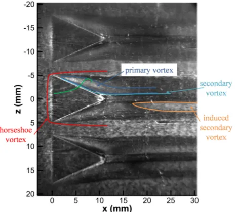
The finer points in the microramp flow topology are surprisingly complex for such a simple geometry [6, 53, 61]. In addition to the primary counter-rotating vortices, the flow topology of a microramp is characterized as having two sets of counter-rotating secondary vortices that are believed to originate in small separation regions at the top edge and wall junction of the ramp trailing edge [17, 50, 53]. Some authors prefer to call these flow structures vortex filaments [6, 53, 61]. An additional set of secondary vortices is induced by the primary vortex tubes near the wall (Fig. 2a). The five-pair vortex model is completed with a horseshoe vortex created from a small leading edge separation that confines the microramp and high-shear region formed by the primary vortex pair downstream of the ramp [6, 17, 50, 53].
Figure 2: Microramp flow structure: (a) time-averaged five-pair vortex model [6, 61], and (b) vorticity distribution in microramp wake [56].
(a)
9
Recently, additional studies on the instantaneous flowfield have added a more detailed explanation regarding the fundamental understanding of microramp flow control [56, 62]. These studies have incorporated such tools as stereoscopic and tomographic particle image velocimetry (PIV) [2, 56] together with implicit large eddy simulations (ILES) [61-63]. The first example of a more complex flowfield was observed by Blinde et al. [2] with the use of stereoscopic PIV in planes parallel with the wall in the inner and outer boundary-layer regions. As in previous studies, counter-rotating longitudinal streamwise vortex pairs were detected in a time-averaged view. Again, these vortices induced both low-speed and high-speed regions downstream of the microramp vertex and intermediate spanwise locations, respectively. Instantaneously, however, the streamwise vortices were not detected. Instead wall-normal vortex pairs, reminiscent of hairpin vortex legs were revealed in the cross plane. A model was conjectured with a train of large-scale hairpin vortices developing downstream of the microramp in the low-speed region [2]. This model is similar to the naturally occurring hairpin vortices observed around the low-speed streaks of a turbulent boundary layer [64].
The three-dimensional flow organization in the wake of a microramp has been further illuminated with the use of tomographic PIV [56]. Qualitatively, the measurements agree with the mean flow of the studies previously described. The circular streamwise velocity wake was bounded by a shear layer at its outer edge, with the counter-rotating vortex pair contained within the wake. Both the wake and vortices are lifted when traveling downstream due to the positive lift force of the induced upwash. The extent of the downwash region was larger with approximately half the intensity as the upwash region. Boundary-layer velocity profiles distinguished the difference in velocity gradients between the upper and lower shear layers of the velocity deficit. A train of arc-shaped vortices wrapping over the trailing counter-rotating vortex pair was revealed in the instantaneous flow structure (Fig. 2b). It is believed that the arc-shaped vortices are generated by a Kelvin-Helmholtz instability occurring in the shear layer surrounding the velocity deficit [6, 56, 61]. The instability in the shear layer is likely aggravated by symmetry breaking as the two primary vortices impinge on one another [6]. Evidence of such ring, or hairpin, vortices is also provided through implicit large eddy simulations [6, 61, 62]. The tomographic PIV results characterized these vortices as arc-vortices due to the lack of data in the near wall-region. Additional laser-light visualization experiments have also revealed similar flowfield structures [54]. A nanoparticle-based planar laser-scattering technique has highlighted that at the microramp trailing edge, the primary vortex pair maintains a coherent round cross section. In this region the wake lifts off rapidly. By approximately 4δ downstream of the ramp, the coherent structure has broken down into the complex train of large-scale hairpin-like vortices. Thus, the authors hypothesize that the basic flow pattern is established by the counter-rotating vortex pair and maintained by the dynamics of the large-scale hairpin vortices [65]. Instantaneously, the streamwise vortices tend to approach each other under the clockwise-rotating
10
ring vortices due to an ejection event. Each ring vortex produces a local high-speed and low-speed region outside and inside the wake, respectively. These studies highlight the complexity of the flow inside the wake due to the interaction between the streamwise vortices and ring vortex train.
Although recent insight into the flow physics of the microramp wake has been offered, the exact mechanism involved in its control of SWBLIs has not been discovered [6]. Numerous studies reveal the overall effectiveness of microramps without providing or fully understanding the working principles of a microramp-controlled SWBLI. The interaction between the microramp vortex pattern and the separated shock system of a SWBLI is likely a very complex vortex/shock interaction that is not as simple as originally reasoned prior to the discovery of the vortex ring pattern [6, 65].
As was previously mentioned in the study by McCormick [16], microramps have been shown to reduce separation and improve boundary-layer characteristics and static pressure recovery downstream of a shock wave. Both transonic normal, or near normal, shock waves [5, 18-21, 66] and supersonic oblique shock waves [2, 15, 17, 58, 59, 65] impinging on the boundary layer have been controlled using microramps. To date, only one research group has focused on ramp-induced shock interactions [6, 61, 63]. Additional studies have also displayed the ability for microramps to reduce shock-induced separation [17-19, 66]. Implicit Large Eddy Simulation methods have been found to have substantial prediction improvements compared with RANS results for these types of SWBLI investigations [59]. The same study found that the microramps tend to increase the boundary-layer thickness behind their centerline, with an overall improvement in boundary-layer health. The smaller microramp devices yielded an improved total pressure recovery and had a greater impact at reducing separation when placed closer to the shock interaction. Lee et al. [59] attributed this effect to decreased wave drag with the smaller device and increased vortex strength through proximity of the device to the SWBLI. The smaller vortices produced by the smaller device were also observed to stay closer to the wall [59]. The drag from the microramp device was determined to be negligible and non-detrimental as described by the difference in the stagnation pressure recovery factor compared to the no-control case [19]. The study of Mach number effects on microramps has revealed that the streamwise vortices decay faster at lower Mach number, possible necessitating larger devices at lower Mach numbers [60]. The spanwise spacing between vortex cores also increases with decreasing Mach number.
Blinde et al. [2] determined the size of the reversed flow region in a controlled oblique shock wave/boundary-layer interaction using stereo PIV. The microramps created a spanwise variation in the SWBLI flow reversal, breaking up the separation regions. A conceptual sketch of the SWBLI was developed upon which the extent of the separation region is based on the mean velocity distribution within the incoming boundary layer. This model has similarities to the instantaneous structure of an
11
oblique shock impinging on a turbulent boundary layer [30]. Specifically, downstream of the microramp vertex, in the low-speed wake region, the flow becomes sonic farther upstream, while the opposite trend occurs in the high-speed region between ramps. Overall, a 20% reduction in the probability of reversed flow at 0.1δ away from the wall was observed. However, the conclusion that the microramps enhance separation in their direct wake is converse to the conclusions reached in other studies [19, 65]. In such a study, Bo et al. [65] found a similar averaged shock foot and separation line undulation based on the velocity distribution of the modified incoming boundary layer. However, the strongest control effect appears in the direct wake of the microramp, beside the center plane, with a large region of reverse flow in the span between. An additional momentum deficit zone is present directly behind the center of the microramp; nevertheless, at the SWBLI the extent of the momentum deficit in the spaces between the microramps is greater. This more accurately corresponds to the high- and low-speed regions produced in the wake of a microramp device. The energized portions of the boundary layer are able to reduce the separation. Similar patterns of separation have been detected in ILES studies [19]. Bo et al. also found that the hairpin, or ring vortices, survive passing through the SWBLI with clearly measured shock distortions and high frequency fluctuations [65]. These shock distortions have also been observed using ILES in the control of ramp-induced SWBLIs [6, 61]. The added benefit of a second row of staggered microramps has also been measured in the control of a SWBLI [2].
In this chapter, a normal SWBLI is characterized in a supersonic blow-down tunnel facility both with and without microramp flow control. The geometry of the microramp is chosen based on the reduction of the transformed form factor through an oblique SWBLI [15]. The microramp array was investigated in a Mach 1.4 flow, for which the SWBLI is incipiently separated. The flowfield is analyzed using instantaneous schlieren photography, surface oil-flow visualization, pressure-sensitive paint (PSP), and particle image velocimetry (PIV). Both time-averaged and instantaneous aspects of the microramp wake and SWBLI are characterized.
2.2 Experimental Arrangement
The microramp characterization experiments were performed in a supersonic blow-down wind tunnel designed for Mach 1.4. The wind tunnel is shown schematically in Fig. 3 and has a test section with cross-sectional area of 63.5 × 63.5 mm (2.5 × 2.5 in). The tunnel is presented with the flow direction from left to right. The wind tunnel facility is capable of generating Mach numbers of 1.4, 1.7, 2.25, and 3 with interchangeable converging-diverging nozzle blocks. The test section has a length of 416 mm (16.4 in). The air supply for the wind tunnel is an Ingersoll-Rand compressor with a 34 m3/min flow rate at 1 MPa pressure. From the compressor, the flow is filtered, dried and cooled before entering a 140 m3 tank farm. The tunnel stagnation pressure is controlled by both a pneumatic valve, with a Fisher TL 101 process
12
controller, and a manual gate valve. After passing through the stagnation chamber, the air accelerates through the converging-diverging nozzle to a nominal freestream Mach number (M∞) of 1.4. The tunnel exhausts through a subsonic diffuser, perforated duct, and exhaust muffler to atmospheric pressure [67]. The wind tunnel is capable of running longer than 20 min. There are three pressure transducers: one for the supply tank, one for the tunnel stagnation pressure, and one for the static pressure in the test section. The supply tank and tunnel stagnation pressure measurements are made with Ashcroft K1 transducers with 1% full-scale accuracy. The static pressure measurements in the test section are made with an Omega PX209-015A5V transducer with 1.5% full-scale accuracy. A thermocouple mounted in the contraction section of the tunnel measures the stagnation temperature. The tunnel has windows in each side wall (107.95 mm × 228.6 mm), providing optical access for schlieren photography, surface oil-flow visualization, pressure-sensitive paint (PSP) and particle image velocimetry (PIV) measurements. A small 50.8 mm (2 in) diameter window was placed in the top wall for additional surface oil-flow visualization and PSP measurements. The top and side windows were fabricated from BK-7 grade A glass. An additional Lexan insert was used along the bottom surface for PIV laser sheet access (Fig. 3). The Lexan material allowed good transmission of the laser light, reducing reflections and allowing resolved measurements closer to the wind tunnel wall.
Figure 3: Experimental schematic showing wind tunnel test section and diffuser.
The stagnation pressure and total temperature of the wind tunnel for this investigation are 247 ± 0.7 kPa (35.9 ± 0.1 psi) and 302 ± 1 K, respectively. The stagnation pressure and temperature ranges are due to small fluctuations throughout the duration of a wind tunnel run. The incoming Mach number (M∞) was
measured to be 1.42 ± .02 using PIV measurements and adiabatic relations. Stagnation and static pressure isentropic relations calculated the Mach number to be 1.38 ± .02. The difference is likely due to non-isentropic boundary-layer losses through the wind tunnel nozzle and test section. The incoming boundary layer is 4.78 ± .15 mm thick, as determined by PIV, and the unit Reynolds number is 38.6 ± 1 × 10⁶ m–1.
13 2.2.1 Incoming Boundary Layer and Flow Properties
PIV measurements of the incoming boundary layer were conducted in order to accurately determine the incoming boundary-layer parameters of the wind-tunnel test section and to determine the correct microramp sizing. The measurements were performed in an empty test section at the location where the microramp array was to be positioned. The incoming boundary layer is characterized by the values shown in Table 1 and the mean velocity profile displayed in Fig. 4. The boundary-layer thickness (δ) of the incoming flow was determined by the wall-normal distance at 99% of the mean freestream velocity.
Table 1: Incoming Boundary Layer Properties
Parameter Symbol Value
boundary-layer thickness δ 4.78 ± .15 mm
displacement thickness δ* 0.655 mm
momentum thickness θ 0.509 mm
incompressible shape factor H 1.29
skin-friction coefficient Cf 0.0020
wake parameter Π 0.56
A modified wall-wake velocity profile for turbulent compressible boundary layers, as discussed by Sun and Childs in [68], was fit to the mean velocity measurements of the incoming boundary layer. The normalized boundary-layer velocity profile was fit to Equation (1) using the least-squares method
(
)
(
)
(
)
1/ 2 1/ 2 1/ 2 1/ 2 * * 1 1 2(1 ) 2sin arcsin 1 ln ln 1 1 1 cos( )
a a e e e u u u u K u a a K u τ
η
τσ
η
η
πη
σ
− Π = + + − + − − + (1) where(
)
1 2 * 1/ 22 1
arcsin
eCf
u
u
τσ
σ
σ
−
=
, 2 21
2
1
1
2
e eM
M
γ
σ
γ
−
=
−
+
,(
)
*1
1
0.614
ln
/
5.2
2
e wu
u
K
u
τK
δ
τν
aK
Π
=
−
−
+
(2)(
)
2 * 1/ 2 2 22
arcsin
4
e eu
A
B
u
A
B
A
−
=
+
, 1 2 21
2
e w eM
A
T
T
γ
−
=
, 2 1 1 2 e 1 w e M B T Tγ
− + = − (3) yη
δ
= , K = 0.41, a = 1 or ∞ (4)The Crocco-Busemann relation (Equation (5)) was used with a recovery factor of r = Pr1/3 to estimate the adiabatic-wall temperature, where Pr is the Prandtl number [69].
14 2 2 e aw e p u T T r c = + (5)
The values of Cf and δ are determined by the curve fit. The value of δ determined from the modified-wall
wake profile corresponds to the wall-normal distance at 99.5% of the mean freestream velocity. The comparison of the modified wall-wake velocity profile to the experimental measurements for the incoming boundary layer is shown in Fig. 4. The boundary-layer incompressible displacement thickness, momentum thickness, and shape factor were calculated using Equation (6) [69].
* 0
1
eu
dy
U
δδ
=
−
∫
, 01
e eu
u
dy
U
U
δθ
=
−
∫
, *H
δ
θ
=
(6)The resulting velocity profile fit in normalized outer coordinates (y/δ and u/U∞) is shown in Fig. 4a.
The incoming boundary-layer profile in wall coordinates (Equation (7)) is what would be expected for a fully developed compressible turbulent boundary layer, as shown in [70], for comparable Reynolds numbers (Fig. 4b) [71]. u u uτ + = , w yu y τ
ν
+ = , 1/2 w wu
ττ
ρ
=
, 2 1 2 w eu Ce fτ
=ρ
(7)In Equation (7), ρw was calculated using the Ideal Gas Law assuming a constant static pressure throughout
the boundary layer and the adiabatic wall temperature calculated from Equation (5). The corresponding friction velocity from the modified-wall wake fit is uτ = 15.4 m/s The Reynolds number based on
incompressible momentum thickness for the incoming boundary layer is Reθ = ρeueθ/µe = 1.97 × 10
4 . The wake strength parameter for the incoming boundary layer is comparable to Π ≈ 0.55 ± 0.05 for a compressible turbulent boundary layer with Reθ > 2000 [69, 70]. The skin friction coefficient for the
incoming boundary layer (Cf = 2.0 × 10
–3
) is also quite similar to that observed for turbulent compressible boundary layers, as described in [68], and the incompressible shape factor compares well with that for a fully developed turbulent boundary layer at Reδ2 = ρeueθ/µw = 1.53 × 10
4
[71, 72].
Figure 4b includes the log law fit from Equation (8), indicating that the resolved log region of the boundary layer approximately covers nine measurement points between 560 < y+ < 1600, which corresponds to 0.15 < y/δ < 0.44 [71]. Due to reflections of the PIV laser sheet along the surface of the wind tunnel, the closest measurement point to the wall is at y+ = 561 (y = 0.72 mm). The lack of resolved measurements in the log region of the boundary layer produces uncertainty in the skin friction coefficient calculations, which is why Cf is only presented to two significant figures rather than three, as specified in
15 1 ln 5.2 u y K + = ++ (8)
Figure 4: Measured incoming boundary-layer velocity profile compared with the fit for a modified wall- wake velocity profile: (a) in normalized outer coordinates and (b) in wall coordinates (BL: boundary layer).
The turbulence intensities of the freestream are less than 1% of the freestream velocity. Figure 5 shows the wall-normal profiles of the turbulent fluctuations compared with planar PIV data of undisturbed compressible boundary layers from Sun [56] and Humble [30], and an incompressible boundary layer measured using hot-wire anemometry from Klebanoff [73]. The root mean square (RMS) fluctuating velocity components, uʹ and vʹ, are normalized by the friction velocity in Fig. 5. The incompressible and compressible data are compared by normalizing the data by the density ratio (ρe/ρw)
1/2
according to Morkovin’s hypothesis. The boundary-layer thickness used for the normalization in Fig. 5 was determined by the wall-normal distance at 99.9% of the mean freestream velocity. The fluctuations of the streamwise velocity component (uʹ) agree well with those for compressible turbulent boundary layers, while having mostly higher values compared to the incompressible boundary layer. This is true except near the outer region of the boundary layer. The wall-normal fluctuations (vʹ) also correspond well with those for compressible turbulent boundary layers. However in this case, the largest difference between the data sets occurs in the near-wall region with the compressible results yielding lower values than the incompressible results. The differences between the measurements may partially be attributed to the limited validity of the scaling in addition to measurement uncertainty. A summary of the relevant test section parameters for this investigation are listed in Table 2.
16
Figure 5: Scaled turbulence intensity comparison for incoming boundary layer [30, 56, 73].
Table 2: Summary of Experiment Test Conditions
Parameter Symbol Value
stagnation pressure po 247 ± 0.7 kPa
static pressure p∞ 80.0 ± 0.7 kPa
boundary-layer thickness δ 4.78 ± .15 mm
freestream Mach number M∞ 1.42 ± .02
freestream velocity U∞ 418.5 ± 4 m/s
stagnation temperature To 302 ± 1 K
freestream temperature T∞ 215.3 ± 1 K
incompressible shape factor H 1.29
skin-friction coefficient Cf 0.0020
unit Reynolds number Re∞ 38.6 ± 1 × 10
6 m–1
2.2.2 Experimental Configuration
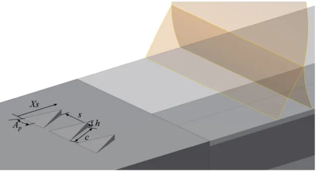
A schematic of the microramp array positioned along the bottom wall of the wind tunnel is displayed in Fig. 6. The normal shock position is included in the schematic. The dimensions used for the microramp array examined were based on the optimized geometries from [15] and are listed in Table 3, as well as shown in Fig. 6. These dimensions were obtained by minimizing the transformed shape factor (Htr) as
explained in [15], based on a design-of-experiments response surface methodology study of 27 unique computational fluid dynamics (CFD) cases varying the Ap, h, c, s, and Xs parameters of the microramp
array. The CFD simulations used the Reynolds-averaged Navier-Stokes WIND code with a grid containing 263,552 mesh points [15].
17
Figure 6: Schematic of microramp array in test section with normal shock wave. Table 3: Microramp dimensions
Parameter Value Physical Dimensions
δ 4.78 ± 0.15 mm -- Ap 24.0° -- h/δ 0.36 h = 1.7 mm c/h 7.20 c = 12.24 mm s/h 7.50 s = 12.75 mm Xs/δ 15.94 Xs = 70.0 mm
The microramp array was machined into an insert that could be replaced with a blank for measurements of the normal shock/boundary-layer interaction without the microramp array. The normal shock was held in place with a 5 deg expansion of the upper wind-tunnel wall that continued for 114.3 mm in the x direction before ending with a lip; this expansion is referred to as the shock holder. The shock holder location with respect to the wind tunnel is shown in Fig. 3. The shock holder held the normal shock at an average Xs/δ value of 14.64 (dimensionally, 70.0 mm), from the leading edge of the microramp array to the normal shock bifurcation point, with a standard deviation of 3.7 mm. The target Xs/δ value was 15.94. This is an 8% difference in shock location from the design value. However, effects of the microramp array are not strongly sensitive to such small changes in shock location, and a complete sensitivity analysis on the effects of varying normal shock position is outside the scope of the current investigation [17]. Without the microramp array, the normal shock was held with a standard deviation of 4.8 mm, and the average shock position moves downstream to x = 79.2 mm.
The effects of the microramp array on the flowfield were evaluated using instantaneous schlieren imaging, surface oil-flow visualization, PSP, and PIV measurements. The investigated regions of the
18
flowfield include the microramp array and SWBLI, in addition to the region downstream of the normal shock wave. The origin of the coordinate system for the measurements presented is located at the center span of the microramp array leading edge. The streamwise, wall-normal, and spanwise coordinate axes are x, y, and z, respectively.
2.2.3 Schlieren Photography
The schlieren optical setup was in a standard Z arrangement (Fig. 7a). Schlieren photography was performed to qualitatively visualize the effects of the microramp array on the boundary layer. Instantaneous schlieren photography also provides a means by which to measure the change in normal shock shape, position, and fluctuations due to the VGs. The instantaneous schlieren photography was conducted using a Newport Corporation flashlamp model LM-1 pulsed at 10 Hz for a duration of approximately 20 ns, a Quantum Composers model 9514 pulse generator, and a Xenon Corporation Nanopulser model 437B. An iris was positioned in front of the flashlamp, effectively creating a point source of light, while the short duration of the flashlamp essentially froze the turbulent structures of the flowfield. The pulsed light was reflected through the test section using collimating mirrors and then focused to a point that is positioned at a knife edge. Both collimating mirrors had a focal length of 1.6 m.
Figure 7: Schematic of flow visualization setups: (a) Schlieren photography and (b) surface oil-flow visualization.
19
The collimated light was aligned perpendicularly, both horizontally and vertically, to the wind tunnel test section. The image was cut horizontally from below with a knife edge before passing into the PCO.1600 charge-coupled device (CCD) camera manufactured by Cooke, Inc. The resolution of the camera was 1600 × 1200 pixels. A photodiode was used to determine camera and flashlamp timing with the pulse generator [74].
The instantaneous schlieren images were processed with a MATLAB script to remove window imperfections and improve image quality. The image background (flow off, light source off) and flatfield (flow off) were acquired prior to each wind tunnel run. The MATLAB script averaged 100 background and flatfield images before subtracting the averaged background from the run image (wind on) and average flatfield image. The program then divided each instantaneous run image by the result of the averaged flatfield minus the averaged background. The presented schlieren images were transformed to the physical xy plane using a first-order linear mapping and scale shot. The schlieren images’ normalized intensity levels are set at arbitrary levels that improve image contrast and display.
2.2.4 Surface Oil-Flow Visualization
Surface oil-flow visualization is a long-standing technique for studying the local flowfield of VGs [53, 75, 76]. The method is used for visualizing the local near-wall flow topology around the microramp array and SWBLI. A schematic of the surface oil-flow visualization setup for visualizing the microramp array region is shown in Fig. 7b as a side-view schematic. The oil used for the surface flow visualization is one part oleic acid, five parts titanium dioxide, and 10 parts silicone oil. Images of the microramp and surface oil flow were obtained through the window in the top of the wind tunnel, while the images of the shock/boundary-layer interaction region were acquired through the large side windows. The same PCO.1600 CCD camera used for schlieren photography was used to obtain the surface oil-flow visualization images. The bottom wind tunnel wall was painted black prior to the application of the oil. The oil was applied generously with a standard foam brush. The brush lines were oriented in the streamwise direction, and images were acquired shortly after the start of the tunnel.
The surface flow images were mapped to the physical xz plane using three linear mapping equations (Equation (9)), where i and j are pixel coordinates and x, y, and z are physical coordinates.
x = a1i+a2j+a3, y = const., z = b1i+b2j+b3 (9) The mapping coefficients were determined from a linear least-squares curve fit from pixel locations to physical coordinates located through a scale shot.
20 2.2.5 Pressure-Sensitive Paint
Pressure-sensitive paint (PSP) measurements allow non-intrusive and high spatial resolution static pressure measurements of the microramp array and SWBLI regions [77]. The pressure-sensitive paint used is composed of an oxygen-sensitive fluorescent molecule (luminophore) and an oxygen permeable binder, specifically, Platinum tetra(pentafluorophenyl)porphine (PtTFPP) in Fluoro/Isopropyl/Butyl (FIB), or Uni-Fib, manufactured by Innovative Scientific Solutions, Inc. PSP measurements function on the principle of oxygen-quenching luminescence from the paint. Namely, when a luminescent molecule absorbs a photon, it is excited to a high energy state, upon which it can return to the ground state with either the emission of a photon of a longer wavelength or a non-radiative interaction with an oxygen molecule (quenching). With a higher oxygen partial pressure, quenching is higher and the luminescent molecules emit less total light [77].
Images of the microramp array and PSP intensity signal were obtained with a similar setup as the images for the surface flow visualizations (Fig. 7b). The microramp array and bottom wind tunnel wall were coated with the Uni-Fib PSP. The paint was excited using a blue LED array (ISSI LM-2 Lamp) with an emitted wavelength of 470 nm. Images of the PSP signal were acquired with a PCO.1600 CCD 14 bit camera fitted with a 610 nm long-pass filter to remove the incident, excitation light. Thus, only the luminescent signal was collected. A series of wind-on images, wind-off (reference) images and background images was acquired both with and without flow control in the regions of interest. The images of the microramp array were obtained with an exposure time of 300 ms. A longer exposure time of 2 s was required for adequate PSP intensity in the SWBLI region. The image intensities were increased by using 2 × 2 binning that reduced the image resolution to 800 × 600 pixels. The image sequences were acquired for approximately 15 minutes, resulting in a total ensemble of 50 microramp array images and 7 SWBLI region images. Each wind-on, wind-off, and background sequence was ensemble-averaged in an effort to reduce shot noise. The average background image was subtracted from the wind-on and reference images to remove any background noise from the images. The wind-on and wind-off images were aligned using a MATLAB script to compensate for any wind tunnel displacement between image acquisitions. The MATLAB script used intensity-based image registration to align the images. Indicated regions of the images were iteratively aligned using translational image transformations. The average translational displacement from these regions was used to align the wind-on and wind-off images. The intensity ratio (Iref/I) of the images was calculated by dividing the wind-on image by the wind-off image, and was used for the calibration of the paint.
Five pressure-tap holes were positioned in and near the microramp array, in addition to along the normal shock/ boundary-layer interaction region. The locations of the pressure taps, both around the