Statistical Inference on Optimal Points to Evaluate Multi-State Classification Systems

(1)

Air Force Institute of Technology

AFIT Scholar

Theses and Dissertations

Student Graduate Works

9-18-2014

Statistical Inference on Optimal Points to Evaluate

Multi-State Classification Systems

Katherine A. Batterton

Follow this and additional works at:

https://scholar.afit.edu/etd

This Dissertation is brought to you for free and open access by the Student Graduate Works at AFIT Scholar. It has been accepted for inclusion in Theses and Dissertations by an authorized administrator of AFIT Scholar. For more information, please [email protected].

Recommended Citation

Batterton, Katherine A., "Statistical Inference on Optimal Points to Evaluate Multi-State Classification Systems" (2014).Theses and Dissertations. 541.

(2)

STATISTICAL INFERENCE ON OPTIMAL POINTS TO EVALUATE MULTI-STATE CLASSIFICATION SYSTEMS

DISSERTATION

Katherine Anne Batterton, Captain, USAF

AFIT–ENC–DS–14–S–02

DEPARTMENT OF THE AIR FORCE AIR UNIVERSITY

AIR FORCE INSTITUTE OF TECHNOLOGY

Wright-Patterson Air Force Base, Ohio

DISTRIBUTION STATEMENT A:

(3)

The views expressed in this dissertation are those of the author and do not reflect the official policy or position of the United States Air Force, the Department of Defense, or the United States Government.

This material is declared a work of the U.S. Government and is not subject to copyright protection in the United States.

(4)

DISSERTATION

Presented to the Faculty

Graduate School of Engineering and Management Air Force Institute of Technology

Air University

Air Education and Training Command in Partial Fulfillment of the Requirements for the

Degree of Doctor of Philosophy

Katherine Anne Batterton, B.S., M.S. Captain, USAF

September 2014

DISTRIBUTION STATEMENT A:

(5)

DISSERTATION

Katherine Anne Batterton, B.S., M.S. Captain, USAF

Approved:

//SIGNED//

Christine M. Schubert Kabban, Ph.D. (Chairman)

//SIGNED//

Lt Col Richard L. Warr, Ph.D. (Member)

//SIGNED// Kenneth W. Bauer, Ph.D. (Member)

16 Jun 2014 Date 27 May 2014 Date 29 May 2014 Date Accepted: //SIGNED// ADEDEJI B. BADIRU, Ph.D.

Dean, Graduate School of Engineering and Management

25 Jun 2014 Date

(6)

Abstract

In decision making, an optimal point represents the settings for which a classification system should be operated to achieve maximum performance. Clearly, these optimal points are of great importance in classification theory. Not only is the selection of the optimal point of interest, but quantifying the uncertainty in the optimal point and its performance is also important.

The Youden index is a metric currently employed for selection and performance quantification of optimal points for classification system families. The Youden index quantifies the correct classification rates of a classification system, and its confidence interval quantifies the uncertainty in this measurement. This metric currently focuses on two or three classes, and only allows for the utility of correct classifications and the cost of total misclassifications to be considered. An alternative to this metric for three or more classes is a cost function which considers the sum of incorrect classification rates. This new metric is preferable as it can include class prevalences and costs associated with every classification. In multi-class settings this informs better decisions and inferences on optimal points.

The work in this dissertation develops theory and methods for confidence intervals on a metric based on misclassification rates, Bayes Cost, and where possible, the thresholds found for an optimal point using Bayes Cost. Hypothesis tests for Bayes Cost are also developed to test a classification systems performance or compare systems with an emphasis on classification systems involving three or more classes. Performance of the newly proposed methods is demonstrated with simulation.

(7)

For my parents who provided me with the tools, and for Dain who kept me sane enough to use them.

(8)

Acknowledgments

First and foremost, I would like to express my sincere gratitude to my advisor Dr. Christine Schubert Kabban for all of her time and support. I could not have completed this work without her guidance and encouragement. Additionally, I would like to thank Dr. Richard Warr and Dr. Kenneth Bauer for serving on my committee and providing their time and knowledge which directly improved this dissertation. I would also like to express my appreciation to Dr. Richard Martin for his thoughtful feedback. Finally, I would like to thank the Department of Mathematical Sciences at the United States Air Force Academy and the department head, Col John Andrew, for giving me this opportunity.

(9)

Table of Contents

Page

Abstract . . . iv

Dedication . . . v

Acknowledgments. . . vi

Table of Contents . . . vii

List of Figures . . . x

List of Tables . . . xi

List of Acronyms . . . xiii

I. Introduction . . . 1

II. Classification and Optimal Performance . . . 3

2.1 Classification System Families . . . 3

2.2 Receiver Operating Characteristic Curves . . . 5

2.3 Optimal Points . . . 6

2.4 Metrics for Optimal Points . . . 8

2.4.1 The Youden Index . . . 8

2.4.1.1 Parametric Methods . . . 11

2.4.1.2 Nonparametric Methods . . . 12

2.4.2 Bayes Cost . . . 13

2.5 Confidence on Optimal Point Metrics . . . 16

2.5.1 Confidence on the Youden Index and Optimal Thresholds . . . 17

2.5.2 Confidence on Bayes Cost and Optimal Thresholds . . . 21

2.6 Hypothesis Tests for Optimal Point Metrics . . . 24

2.7 Distributions for the Youden Index and Bayes Cost Inference . . . 25

2.7.1 Binomial Distribution . . . 25

2.7.1.1 Confidence Interval for Binomial Proportions . . . 25

2.7.2 Multinomial Distribution . . . 26

2.7.2.1 Confidence Intervals for Multinomial Proportions . . . 27

2.8 Summary . . . 29

III. Parametric Confidence Intervals . . . 31

3.1 Introduction . . . 31

(10)

Page

3.2.1 Bayes Cost and Optimal Thresholds, 3 classes. . . 32

3.2.2 Bayes Cost and Optimal Thresholds,kclasses. . . 35

3.2.3 A Method for Numerically Estimating Partial Derivatives. . . 36

3.3 Generalized Confidence Intervals. . . 37

3.3.1 Youden Index,kClasses . . . 37

3.3.2 Bayes Cost, Equal Weights . . . 39

3.3.3 Bayes Cost, Unequal Weights . . . 39

3.4 Bootstrap Methods . . . 40

3.5 Simulation Results . . . 41

3.5.1 Equal Costs and Prevalences . . . 44

3.5.1.1 Performance of Confidence Intervals around Bayes Cost. . . 44

3.5.1.2 Performance of Confidence Intervals around Optimal Thresholds 46 3.5.2 Unequal Costs . . . 47

3.6 Summary . . . 50

IV. Nonparamteric Confidence Intervals . . . 55

4.2 Fiducial Intervals . . . 55

4.2.1 Bayes Cost with Equal Weights . . . 56

4.2.2 Bayes Cost with Unequal Weights . . . 64

4.2.3 Fiducial Interval around Bayes Cost Algorithm . . . 68

4.2.3.1 General Case. . . 68

4.2.3.2 Special Case: Equal Sample Sizes and Weights. . . 70

4.2.4 Equivalence for the Youden Index . . . 71

4.3 Bootstrap Methods . . . 71

4.4.1 Equal Costs . . . 72

4.4.1.1 No Distributional Assumptions on the System . . . 73

4.4.1.2 Normally Distributed Feature . . . 73

4.4.2 Unequal Costs . . . 78

4.5 Comparisons to Multinomial Methods . . . 79

4.5.1 Simulation Results . . . 81

4.6 Summary . . . 83

V. Parametric Hypothesis Tests . . . 87

5.2 Delta Method Hypothesis Tests . . . 88

5.2.1 One-sided Hypothesis Test on a Single Bayes Cost Value . . . 88

5.2.2 One-sided Hypothesis Test on the Difference of Two Bayes Cost Values . . 89

5.3 Generalized Hypothesis Tests . . . 91

(11)

Page

5.5 Summary . . . 105

VI. Nonparametric Hypothesis Tests . . . 107

6.2 Exact Hypothesis Tests . . . 108

6.3 Likelihood Ratio Tests . . . 110

6.5 Summary . . . 121

VII. Applications . . . 123

7.1 Classifying Breast Cancer. . . 123

7.2 Classifying Chronic Allograft Nephropathy . . . 128

VIII.Conclusions . . . 133

Appendix A: Mathematical Derivations and Support . . . 135

Appendix B: Additional Tables . . . 155

Appendix C: R Code . . . 175

(12)

List of Figures

Figure Page

2.1 Classification System Example . . . 5

2.2 Receiver Operating Characteristic Curve. . . 6

2.3 Different Optimal Points for the Same Classification System Family . . . 8

2.4 Three-Class Classifications for HIV Example . . . 9

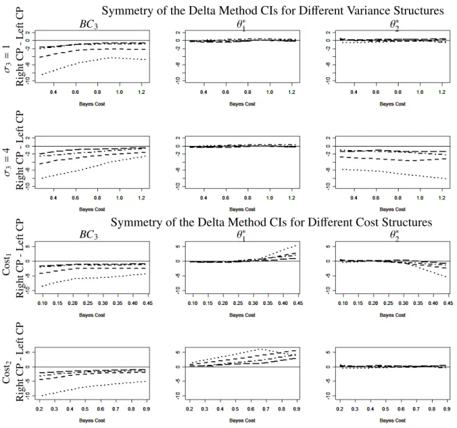
3.1 Symmetry of Delta Method Confidence Intervals . . . 48

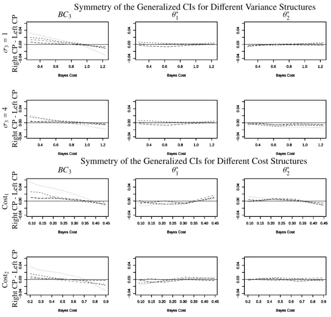
3.2 Symmetry of Generalized Confidence Intervals . . . 49

4.1 Example ofFy(y|p) . . . 62

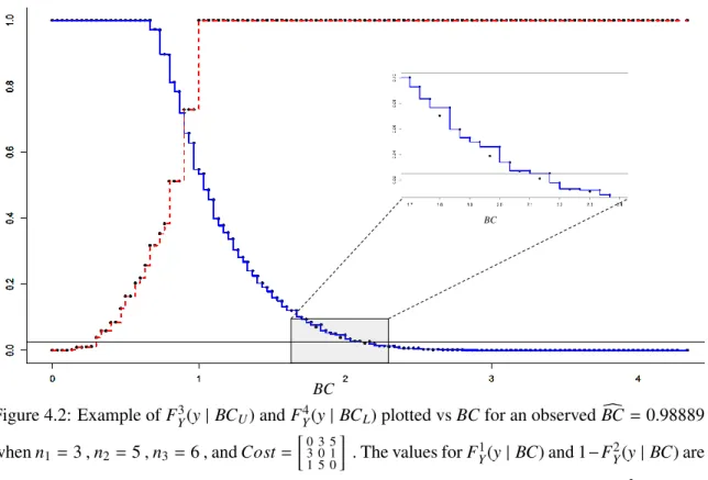
4.2 Example Functions for Fiducial Intervals aroundBC . . . 66

4.3 Simulation Results for Simultaneous Multinomial Confidence Intervals . . . 82

4.4 Minimum Coverage for Fiducial Interval Example. . . 84

6.1 Nonparametric Hypothesis Tests’ Power Curves . . . 119

(13)

List of Tables

Table Page

2.1 Two-Class Contingency Table . . . 4

2.2 Three-Class Contingency Table. . . 5

2.3 Outcomes from a Two-Class Classification System Arranged in a Contingency Table . 26 2.4 Outcomes from ak-Class Classification System Arranged in a Contingency Table . . . 27

3.1 Distributional Parameters for Parametric Confidence Interval Simulation . . . 43

4.1 Example Multinomial Sample Space . . . 58

4.2 Example of Reduction of Multinomial to Binomial Sample Space . . . 59

4.3 Ties in Bayes Cost Sample Space for a Single Experiment . . . 61

4.4 Simulation Results for Nonparametric Confidence Intervals . . . 74

4.5 Distributional Parameters for Nonparametric Confidence Interval Simulation. . . 75

4.6 Simulation Results for Nonparametric Confidence Intervals 1 . . . 76

5.1 Distribution Parameters for Parametric Hypothesis Test Simulation . . . 96

5.2 Simulation Results for Parametric Hypothesis Tests 1 . . . 98

6.1 Simulation Results for Nonparametric Hypothesis Tests 1 . . . 116

(14)

Table Page

6.5 Comparison of Exact and LRT p-values . . . 121

7.1 Descriptive Statistics of Features to Classify Breast Tissue . . . 125

7.2 Contingency Tables for Classifying Breast Tissue . . . 126

7.3 Descriptive Statistics of Features for Classifying Allograft Function . . . 128

7.4 Contingency Tables for Classifying Allograft Function . . . 131

B.1 Simulation Results for Parametric Confidence Intervals 1 . . . 156

(15)

List of Acronyms

Acronym Definition

ADI adipose

AN asymptotic normal

BC Bayes Cost

BCa bias corrected and accelerated BP basic percentile

CAR carcinoma

CDF cumulative distribution function CI confidence interval

CLT Central Limit Theorem

CON connective

CSF classification system family FAD fibro-adenoma

GCI generalized confidence interval

GLA glandular

GPQ generalized pivotal quantity LRT likelihood ratio test

MAS mastopathy

MLE maximum likelihood estimator pdf probability density function pmf probability mass function GYI generalized Youden’s index

J Youden’s index

ROC receiver operating characteristic VUS volume under the surface WLOG without loss of generality

(16)

I. Introduction

Decision making occurs daily in a vast range of fields, from health care to information processing and military applications. Generally, these decisions may be based offof classification systems which, for example, label an individual as diseased or not diseased or perhaps label an object of interest as a target or non-target. Although such decisions could be made as simply as through a quick visual inspection, for many decisions of critical importance it is of interest to use statistics and best practices to develop and compare classification systems and quantify their performance so as to choose the best classification method available to aid such decisions [68].

A simple classification rule may classify an item into one of two classes, such as ”Positive” and ”Negative”, or ”Diseased” and ”Not Diseased”. Although a lot of research has been conducted to develop methods for the quantification of such classification systems, most applications in the real world are more complicated and do not fit into simple binary classification rules. Despite examples of classification systems in most applications, this research focuses on examples from a medical diagnostic standpoint, as medical diagnostics carry great importance as well as the possibility for large consequences with respect to misdiagnoses.

One recent example of a medical diagnostic decision involves the use of biomarkers to diagnose subjects post kidney transplant as either being normal kidney function, normal kidney function with proturina (a progression towards the diseased state), or chronic allofraft nephropathy (the diseased state) [58]. Other examples abound such as that of HIV diagnosis. While screening for this disease by using a specific biomarker, patients can be categorized into one of three categories: HIV-negative, HIV-positive non-symptomatic, and HIV-positive with AIDS dementia complex [45]. Extending the health concept to structures, we may be interested in the detection of the stage of structural

(17)

damage as being none, within a pre-specified safety range, or beyond the safe operating range. In all of these examples the middle class is important as it represents a state in the progression of some phenomenon (e.g. disease or damage). Thus, diagnosis of the middle class may allow for intervention to prevent a subject or specimen from reaching the end state.

There are methods available to determine the performance of a classification system requiring more than two outcomes. Many of these methods use extensions of receiver operating characteristic (ROC) curve theory for comparing classification systems on their abilities to correctly classify objects [16,17,20,28,29]. However, the number of possible outcomes is not the only concern when choosing a classification system. The prevalence of the different classes as well as the costs associated with making the correct (or incorrect) decision should also be considered [30,42,58,65]. For example, in HIV diagnosis, different misclassifications may be considered more or less significant. A person who is misdiagnosed as the non-diseased state when they are actually HIV-positive may be considered much worse than the opposite error occurring (a non-diseased person who is diagnosed as HIV-positive). In the first scenario, a person will not receive necessary medical intervention and may now put others at risk since they are unaware of their HIV-positive status. Clearly though, the latter misdiagnosis presents its own cost in that an individual may begin treatment or otherwise suffer with a diagnosis that is incorrect.

In a two-class setting, assigning a cost to the different misclassifications is equivalent to assigning an associated cost to the different correct classifications. However, this equivalence does not universally exist for settings with three or more classes. Currently, little work has been done to compare and quantify the performance of multi-class classification systems by using the misclassifications. By using the misclassifications, different costs may be placed on all the possible errors made by the classification system [58,65].

The work of this dissertation improves classification system selection and performance quantification for more complicated classification settings involving three or more classes with unequal costs associated with the different misclassification errors. Specifically, precision of estimates of classification system metrics and their optimal points through confidence intervals and hypothesis tests are explored to aid decision makers.

(18)

II. Classification and Optimal Performance

2.1 Classification System Families

A classification system (A) is any process that assigns the elements fromk partitions of an event set,E=(ε1, ε2, ..., εk) tokdistinct elements of a label set,L=(l1,l2, ...,lk).These partitions

may be referred to as classes. For example, a two-class label set could be{0,1}or{Diseased, Non Diseased}. Data is collected on the elements, which are then processed into a feature or set of features,F= (f₁, f₂, ...,fm). These features are then used to assign the different elements fromE

to the respective labels,L,(A:E→F→L).It is assumed that there is a parameter or vector of parameters for the features,θ∈ Θ,that can be altered to change the outcome of the classification system.1 Thus, for everyθ∈ Θ,there is a classification system (Aθ),and the set of classification systemsA = (Aθ,θ ∈ Θ) is called a classification system family (CSF) [58]. It is also assumed that there exists a truth label set,T=(t1,t2, ...,tk),such that all elements of the population would be

correctly labeled by this set.

A two-class classification system has four outcomes with respect to truth (see Table 2.1). Defining one class as positive and the other class as negative, the possible outcomes from the classification system are true positive, true negative, false positive, and false negative. True positive occurs when the system correctly classifies a positive element with a ”positive” label (the rate of true positive is often called sensitivity). True negative occurs when the system correctly classifies a negative element with a ”negative” label (the rate of true negative is called specificity). These two outcomes are correct classifications. The other two outcomes are misclassifications. A false positive occurs when the system incorrectly classifies a negative element with a ”positive” label. Likewise, a false negative occurs when the system incorrectly classifies a positive element with a ”negative” label. The results of a classification system are often arranged in a contingency table as seen in Table2.1with the truth along the columns and the classification results down the rows.

(19)

Table 2.1: Two-class contingency table where green cells correspond to correct classifications and red cells correspond to misclassifications.

Positive Negative

“Positive” True Positive False Positive

“Negative” _NegativeFalse True Negative

TRUTH C L A SSI F IC A T ION

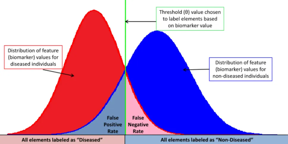
An example classification system in a medical diagnostic setting may have elements in partitions of the event set,E=(Non-Diseased, Diseased), and the label set, L =(”Non-Diseased”, ”Diseased”). After the collection of data such as a patient’s blood sample, the feature extracted might be the value of a specific biomarker determined from the blood sample,F=(biomarker level,

µmol). Then a single threshold,θ ∈ Θ ,is determined so that whenever the observed biomarker level is less than θ , the patient is labeled as ”Diseased”, and whenever the biomarker level is greater thanθ ,the patient is labeled as ”Non-Diseased” (see Figure2.1). For instance, when total cholesterol (a biomarker feature) is greater than 240 (the threshold), a patient may be labeled with ”high cholesterol”.

In the two-class case, there are two correct classifications and two misclassifications. In the k-class case there arekcorrect classifications andk2−kmisclassifications. When there are more than two classes, the correct and misclassifications can no longer be defined as true positive or false negative. Therefore, these terms are generalized to correct classifications and misclassifications. For simplicity of notation, the outcomes are labeledi| j,where jis the true label for an element andirepresents the classification system label for an element,i, j=1,2, ...,k.Then for alli= j, the outcome is a correct classification and for alli, j,the outcome is a misclassification (see Table

(20)

False Positive Rate False Negative Rate Distribution of feature (biomarker) values for

diseased individuals Distribution of feature

(biomarker) values for non-diseased individuals Threshold (θ) value chosen

to label elements based on biomarker value

All elements labeled as “Diseased” All elements labeled as “Non-Diseased”

Figure 2.1: Example of a classification system in a medical setting where elements are either diseased or non-diseased. Hypothetical feature distributions for each class and a potential threshold (green line) used to label the elements as either ”Diseased” or ”Non-Diseased” are shown.

Table 2.2: Three-class contingency table where green cells correspond to correct classifications, i= j, and red cells correspond to misclassifications,i_, j.

CLASS 1 CLASS 2 CLASS 3

“CLASS 1” 1|1 1|2 1|3 “CLASS 2” 2|1 2|2 2|3 “CLASS 3” 3|1 3|2 3|3 TRUTH C L A SSIF IC A TION

2.2 Receiver Operating Characteristic Curves

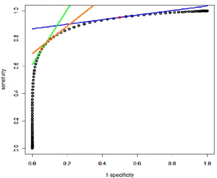
Receiver operating characteristic (ROC) curves are used to describe the performance of a CSF when there are two classes (See Figure2.2). The ROC curve plots the true positive rate versus the false positive rate over all threshold values,θ∈Θ.This curve allows for interpretation of the trade-offbetween the true positive and false positive rates for varying thresholds. Thus, the ROC curve represents the performance of the entire CSF for allθ∈Θ.

(21)

The ROC curve plots classification rates, bounding the curve between 0 and 1 on both the horizontal and vertical axes. The point on the ROC curve that represents perfect classification is (0,1) (Figure2.2). This point represent a perfect true positive rate (1) and a perfect false positive rate (0). Therefore, CSFs whose ROC curve approach this point are desired and the single classification system closest to this point is optimal. In a two-class setting, the probability of correctly classifying due to random chance is 0.5. The line on the ROC plot that corresponds to chance classification is called the chance line and intersects the points (0,0) and (1,1) (Figure2.2) [19]. A CSF performing worse than random chance would not be of interest, and therefore only CSFs whose ROC curves lie above the chance line are usually considered. Finally, when there are more than two classes, the ROC curve may be extended to a ROC surface by plotting the correct classification rates over all

θ∈Θin akdimensional space, though only the 3-dimensional surface is visible graphically.

(1,1)

(0,0) (0,1)

Figure 2.2: Receiver Operating Characteristic Curve.

2.3 Optimal Points

The single classification system resulting in the best classification performance for the CSF is said to occur at the optimal point (or points), corresponding to someθ∈Θ.For a two-class system, the optimal point is usually found where the probability of a true positive and the probability of a true

(22)

negative are maximized (maximization of correct classification probabilities), or equivalently, where the false positive and false negative probabilities are minimized (minimization of misclassification probabilities). Therefore, the optimal point reflects a compromise between the correct classification probabilities (or misclassification probabilities) [42]. The optimal point for a two-class CSF can be found using the ROC curve. If the prevalence of classes and costs associated with classification outcomes are considered equal for both classes, the optimal point occurs where the tangent line to the ROC curve is parallel to the chance line (ie. the slope of the ROC curve is 1) [42]. This is equivalent to finding the point on the ROC curve with the greatest vertical distance from the chance line [54]. The threshold value(s) that produce this point are then chosen as the optimal threshold values for this CSF.

Extensive work in the literature suggests that costs associated with a classification system’s outcomes should be taken into account when evaluating the system and estimating optimal thresholds [1, 30, 42, 58, 63–65,67]. In addition to the costs of the classification outcomes, the prevalence of the different classes may be of importance when determining optimal settings for a CSF [9, 42]. If the a priori prevalence of the diseased and diseased (or target and non-target) classes as well as the a prioricosts associated with the decision outcomes are taken into consideration, the CSF may have a different optimal point (see Figure 2.3) [19, 58, 67]. When prevalence and costs are considered, the optimal point occurs on the ROC curve where the slope is equivalent to S lope= 1−pP pP × " cFP−cT N cFN−cT P # (2.1)

[42]. ThepPis the prevalence of the positive class,cT Nis the cost of a true negative,cFPis the cost of a false positive,cT Pis the cost of a true positive, andcFN is the cost of a false negative. Under the assumption of equal prevalences and equal costs of misclassification (or correct classification), this slope is equal to one as expected.

The optimal point for ak-class classification system will usually correspond to at leastk−1 threshold values. For example, in order to classify subjects into three categories (HIV negative (NEG), HIV positive non-symptomatic (NAS), and HIV-positive with AIDS dementia complex (ADC)), two threshold values (θ1 < θ2) on a biomarker (NAA/Cr) may be used as a diagnostic

(23)

Figure 2.3: Different optimal points (in red) for the same CSF, determined by Equation2.1. The orange line has a slope of one, representing equal class prevalence and costs associated with the classifications. Both the green and blue lines assume a positive class prevalence of 1/3. The blue line has a slope of 1/6 withcFN >>cFP.The green line has a slope of 2 withcFP=cFN .For each linecT N =cT P=1.

test [45]. If a subject’s NAA/Cr level is belowθ1they are classified as ADC, if the subject’s NAA/Cr

level is betweenθ1 andθ2they are classified as NAS, and finally if the subject’s NAA/Cr level is

greater thanθ2they are classified as NEG [45] (see Figure2.4).

2.4 Metrics for Optimal Points

2.4.1 The Youden Index.

The Youden index (J) was first introduced by W. J Youden in 1950 as an index for rating diagnostic tests (or classification systems) with two classes [76]. The Youden index has been shown to be a useful metric for measuring a classification system’s performance as a function of the correct classification probabilities [23,45,46,50,56,76]. In a two-class framework, this index is defined

(24)

1 θ θ2 Classified as NAS Classified as ADC Classified as NEG

Figure 2.4: Three-class classifications for HIV example. Distributions of the NAA/Cr levels are plotted for ADC (black), NAS (red), and NEG (blue) as well as potential threshold values,θ1and

θ2,used to determine a subject’s classification.

as the sum of the system’s specificity (true negative rate) and sensitivity (true positive rate) minus one. UsingJ, the optimal point of the classification system is found by choosing the threshold(s),

θ∈Θ,that maximizeJ, thereby maximizing the correct classification probabilities. The thresholds associated with the maximumJ characterize the CSF at its optimal performance (with respect to correct classification) and correspond to the optimal point on the ROC curve where the slope is equal to one. Therefore, classification systems can be compared by calculatingJ:

J=max

θ∈Θ{sensitivity(θ)+speci f icity(θ)−1} (2.2)

A classification system which performs worse than chance is generally not of interest, and therefore it is assumed that both sensitivity and specificity are bounded between 0.5 and 1. For this reason, J = sensitivity(θ)+speci f icity(θ)−1 is bounded between 0 and 1 for systems performing better than chance [76].

(25)

Costs associated with the different classifications as well as class prevalence may be of importance in the determination of J. In fact, when not explicitly considering a cost structure when usingJ, a cost and prevalence for each class is being assumed, that of equal weight for all classes [55,64]. Other costs may be considered by using a generalization toJwhich incorporates a cost benefit ratio weighted by class prevalence in the two-class framework [30,63]. The generalized Youden index (GYI) for two classes is defined as

GY I =max θ∈Θ ( sensitivity(θ)+ 1−pP pP × " cFP−cT N cFN−cT P # ×speci f icity(θ)−G ) (2.3)

where G is a constant determined by the prevalence of the positive class and the costs associated with the different decisions [30,40,63]. Notice that the prevalence/cost multiplier is the same as in Equation2.1

When there are more than two classes,J is extended as the sum of thekcorrect classification probabilities [45,46]. Under this framework, the correct classification probabilities can no longer be distinguished by sensitivity and specificity, so instead, thek correct classification probabilities are labeled asPi=j|j(θ),where j=1, ...,kdenotes the true class andi=1, ...,kdenotes the classification

system’s labeled outcome. ThenJis redefined as

J =max θ∈Θ              k X i=1 i=j k X j=1 Pi|j(θ)              (2.4)

Jis generalized by adding a multiplier (prevalence and/or utility) to each correct classification probability for classification systems with three or more classes [45, 46]. The limitation with such an extension is that only costs of the total misclassification and (utility of the) total correct classification outcomes within each class are used. This ignores possible different costs on class specific misclassifications. For example, misclassifying stage 3 cancer as stage 2 may have a different cost than classifying stage 3 as stage 1.

Extensive work has derived formulas for determiningJand the optimal threshold(s) for CSFs, under various distributional assumptions of the feature used for classification, and focused on the two-class framework [23,33,49,54,56]. An overview of these results are given in the following sections, and are separated into parametric and nonparametric methods.

(26)

2.4.1.1 Parametric Methods.

Assume two classes and a single feature used for classification where the feature is independently and normally distributed for each class, whereXis the first class andY is the second class, denoteXj ∼ N(µ1, σ2₁) for j= 1, ...,n1,Yi ∼ N(µ2, σ2₂) fori=1, ...,n2,and without loss of

generality (WLOG) letµ1 < µ2 (see Figure2.1). Recall that the probability distribution function

(pdf) for the normal distribution is

f(w|µ, σ)= √1

2πσe

−(w−µ)2

2σ2 − ∞<w<∞, − ∞< µ <∞, σ >0 (2.5)

Then the Youden index may be written as

J = Φ µ2−θ ∗ σ2 ! + Φ θ∗−µ1 σ1 ! −1 (2.6)

whereΦis the normal cumulative distribution function (CDF) [56]. Here, the maximum is excluded because the optimal thresholdθ∗is used. The closed form solution for the optimal threshold,θ∗∈Θ,

which maximizes Equation2.6is given by

θ∗₌ µ1(b

2₋₁₎₋_a₊_bq_a2+₂₍_b2₋₁₎σ2

1ln(b)

(b2₋₁₎ (2.7)

wherea = µ₂−µ₁ andb = σ2

σ1 [56]. Ifσ1 = σ2 ,this result does not exist, but for this case the

optimal point is the midpoint between the distribution means given by [56]:

θ∗₌ µ1+µ2

2 (2.8)

The GYI may also be rewritten using the normal CDF:

GY I = Φ µ2−θ ∗ σ2 ! +R×Φ θ ∗₋_µ 1 σ1 ! −G (2.9) where R= 1−pp pp × " cFP−cT N cFN−cT P # (2.10)

Again, the maximization is excluded because this equation is being evaluated at the optimal threshold. Accounting for fixed class prevalences and costs associated with the classification outcomes, the optimal threshold whenσ2₁=σ2₂is

θ∗₌ 2σ 2_ln(_R₎₋_µ2 1−µ 2 2 2(µ2−µ1) (2.11)

(27)

[30]. Whenσ2₁,σ2₂the optimal threshold is θ∗₌ µ1(b 2₋₁₎₋_a₊_bq_a2+₂₍_b2₋₁₎σ2 1ln(R×b) (b2₋₁₎ (2.12) wherea=µ₂−µ₁andb= σ2 σ1 [63].

When there are three classes, there is an additional class, Z, where Zm ∼ N(µ3, σ2₃) for

m = 1, ...,n3 . J is then defined as the sum of the three correct classification probabilities and

can be expressed using the normal CDF as

J= Φ θ ∗ 1−µ1 σ1 ! + Φ θ ∗ 2−µ2 σ2 ! −Φ θ ∗ 1−µ2 σ2 ! −Φ θ ∗ 2−µ3 σ3 ! +1 (2.13)

whereθ∗₁< θ∗₂are the optimal thresholds found to maximizeJ[45]. The solutions for these optimal thresholds can be found with Equation2.7where the solution forθ∗₁is found witha= µ₂−µ₁and b = σ2

σ1 .The solution forθ ∗

2 is found similarly witha = µ3−µ2 andb =

σ3

σ2 [36]. Although the

GYI has not been extended for three classes, in [45] the three-classJis generalized with weights on each correct classification probability. Therefore, weights could be added to Equation2.13and the optimal thresholds (θ∗₁< θ₂∗) would be found numerically.

Finally, for all forms ofJand GYI, if the classification feature is distributed log-normally, the point estimate of the threshold is determined using log-transformed data. A similar development is presented in [56] forJ with two classes and a gamma distributed feature. However, for features distributed within the Box-Cox family, transformations to normality may be used and the formulas assuming normality applied [30,45].

2.4.1.2 Nonparametric Methods.

For any number of classes, if no distributional assumptions about the feature used for classification are made, J can be defined using the empirical CDF. The empirical CDF, Fn(x) , of a random sample of sizenis defined as

Fn(x)= 1 n n X i=1 I(Xi ≤ x) (2.14)

whereI is the indicator function and is equal to 1 if the relation is true, and 0 otherwise [32]. For example, in a three-class scenario (X<Y <Z),Jmay be defined as

J= Fb(θ ∗ 1)+Gb(θ ∗ 2)−Gb(θ ∗ 1)−Hb(θ ∗ 2)+1 (2.15)

(28)

where Fb(θ) = _n1 1 Pn1 i=1I(xi ≤ θ) , Gb(θ) = _n1 2 Pn2 j=1I(yj ≤ θ) , Hb(θ) = _n1 3 Pn3 m=1I(zm ≤ θ) , and θ∗ 1 andθ ∗

2are the thresholds found to maximize Equation 2.15[45]. Methods that have been used

to determine the optimal thresholds include a smoothing kernel method on the empirical CDFs, choosing the observations where the maximum occurs, or by random walks [45,63].

All forms of J presented may be extended for the k-class J, where again, weights may be placed on the correct classification probabilities to incorporate the importance of the different correct decisions in finding the optimal point [46]. Other work on J includes consideration of special cases such as pooled samples, corrections for measurement error, and methods for when the feature distribution has a mass at zero [49,54,55].

2.4.2 Bayes Cost.

The optimal threshold found by maximizing the correct classification probabilities (via J) is equivalent to that found by minimizing the misclassification probabilities in a two-class framework [6, 50]. When there are more than two classes and unequal costs associated with the misclassifications within each class, the equivalence between optimal thresholds found by maximizing correct classification probabilities and minimizing misclassification probabilities is not universally true. This is because it is no longer feasible to assign a simple cost benefit ratio between the benefit of making a correct decision and the costs of making an incorrect decision [58, 65]. Therefore, finding the optimal settings can be more complex when a classification system has more than two classes. In order to assign differing costs or benefits to the potential outcomes of ak-class classification system, a metric that considers all differing misclassification probabilities should be considered instead of extensions ofJ.

Ak-class classification system results in a total ofk2correct classification and misclassification probabilities; however,J only uses k pieces of information (kcorrect classification probabilities). Therefore, by usingJ, k2 −k pieces of information about the classification system may be lost, namely information about the class-specific misclassifications. A metric developed on the k2 −k error probabilities will lose no information about the system [58] (see Theorem1).

For this reason, the development of a metric associated with the misclassification probabilities is of interest. Bayes Cost (BC) is a metric presented in [65] that minimizes misclassification

(29)

probabilities for three or more classes. This metric allows for misclassification probabilities to be weighted by the cost and class prevalence associated with each misclassification outcome.

Bayes Cost=min

θ∈Θ              k X i=1 i,j k X j=1 ci|jpjPi|j(θ)              (2.16)

where ci|j is the fixed cost associated with misclassifying class j as class i and pj is the fixed prevalence for the jthclass. Therefore,BC allows for the use of any cost/prevalence structure on both the correct and misclassification probabilities.

Theorem 1. Using Bayes Cost to determine the optimal thresholds of a multi-state classification system allows for the use of any cost/prevalence structure on any of the correct or misclassification probabilities, therefore not losing any information about the classification system.

Proof. Let the prevalence of the class be denoted pj and the cost of a misclassification be mi,j|j or benefit of a correct classification be bi=j|j, where the true class is denoted j = 1,2, ...,k and classification outcomes are denoted i=1,2, ...,k. The cost function to minimize would be

Cost=min θ∈Θ          k X i=1 k X j=1 pjmi,j|jPi,j|j(θ)+ k X i=1 k X j=1 pjbi=j|jPi=j|j(θ)          (2.17)

Note, since the classification outcomes in each class are mutually exclusive and the sample size of each class (nj) is fixed:

k X i=1 Pi|j(θ)=1, for each j=1,2, ...,k (2.18) which implies Pi=j|j(θ)=1− k X i=1 Pi,j|j(θ), for each j=1,2, ...,k (2.19)

(30)

= Bayes Cost+constant

=⇒ θ_Cost∗ =θ∗_BC

(2.20)

This demonstrates that the optimal thresholds found by minimizing Bayes Cost are equivalent to those found by minimizing a function which uses all classification outcome probabilities from the classification system, allowing for any cost/benefit and prevalence structures to be considered.

Assume a three-class classification system with a single feature used for classification that is independently and normally distributed for each class, whereµ1< µ2< µ3.Under this framework,

BC can be expressed with the standard normal CDF and the optimal thresholds that distinguish between the classes and minimizeBC,θ∗₁< θ∗₂,as:

The minimization is not expressed in Equation 2.21 as this is achieved by using the optimal thresholds. The optimal thresholds must be found numerically when all ci|jpj are not equal, for i, j. When allci|jpjare equal, fori, j,Equation2.7may be used to find the optimal threshold

(31)

between each set of normal distributions. Equation2.21may be extended for anyk classes with a single feature used for classification that is independently and normally distributed for each class, and would requirek−1 optimal thresholds.

When there are two classes, the optimal threshold found by minimizingBCis equivalent to that found by maximizing the GYI, Equations2.11or2.12(assuming the same costs and prevalences used to find the optimal point). A proof of this equivalence is given in Section2.5.2. Also, if all ci|jpj are equal, fori , j, the optimal threshold(s) found with BCwould be equivalent to those

found by maximizingJ.

In a nonparametric setting, BC can be estimated using the empirical distribution function. Lettingθ= (θ1 < θ2 < ... < θk) andFj be the empirical CDF for the jthclass withFj−1 < Fj,for allkclasses,BCis defined as

BC =min θ∈Θ              k X i=1 i,j k X j=1 ci|jpj h Fj(θi)−Fj(θi−1) i              (2.22)

where Fj(θ0) = 0 and Fj(θk) = 1 [65]. The optimal thresholds are then found to be those which

minimize Equation2.22.

2.5 Confidence on Optimal Point Metrics

It is critical to characterize the uncertainty in an optimal point, as such estimates are typically constructed from data. This is most commonly accomplished by creating confidence intervals (CIs) around the metric used to characterize the optimal point (Youden index, Bayes Cost, etc) as well as creating confidence interval(s) around the threshold(s) which correspond to the optimal point [30,33,49,56,76].

CIs are a statistical inference method that provide a range of values (usually an interval) for which there is a specified level of confidence that the true parameter lies within the interval. CIs may be constructed as either one or two sided (one sided being of the form where there is either a lower or upper bound, but not both). This work focuses on constructing two sided confidence intervals. If X = (X1, . . . ,Xn) is a random sample, then L(X) and U(X) form a confidence

interval with confidence coefficient 1−αfor some function of the parameter θ , τ(θ) , such that P[L(X) ≤ τ(θ) ≤ U(X)] = 1− α[12, p. 417],[44, p.377]. Because it is known that the upper

(32)

and lower bounds of the CI are functions of the observed data, the notation for the bounds may be simplified by writingL(X) asτ(θ)LandU(X) asτ(θ)U.

Not all CIs perform equally well. An interval’s coverage probability and length are metrics of a CI’s performance. If a CI with a confidence coefficient of 1−αis constructed 100 times, it is expected that (1−α)100% of the intervals actually contain the true parameter of interest. This may not always be the case, and the percent of constructed CIs that contain the true parameter is the coverage probability of the CI. The coverage probability should be at least (1−α)100% for a well performing CI. CIs with coverage probability greater than (1−α)100% are considered conservative. For all CIs that meet the desired coverage probability, it is then of interest to find the interval with the shortest length. The length of an interval is defined asτ(θ)U−τ(θ)L.A shorter length CI which meets the desired coverage probability provides a more precise (and therefore, arguably, a more useful) estimate of the parameter. Another metric of CI performance is its symmetry, which may be used to judge whether or not the true parameter of interest lies in the center of the interval, or if the interval is skewed to one side. Mean squared error and bias of the parameter estimate may impact CI performance and are therefore also sometimes considered, though these are not properties of the interval itself.

2.5.1 Confidence on the Youden Index and Optimal Thresholds.

Several methods exist in the literature for constructing CIs around J and the optimal threshold(s), mainly in a two-class setting. In addition to these methods, bootstrap methods are also applicable, as bootstrap CIs are a general and flexible method that may be used under any distributional assumptions of the features and classification system structure. First, parametric CI methods are presented and following these methods, the nonparametric CI methods available forJ are presented.

A delta method approximation, which uses first order Taylor series expansions to determine the variance of J and the optimal threshold(s), has been implemented to create CIs for J and the resulting optimal threshold(s) for a classification system with two or three classes with a single feature that is independently and normally distributed for each class [36,56, 63, 64]. The delta

(33)

method (1−α)100% CI aroundJis b J±zα/2 q VarJb (2.23)

where Jbis estimated using Equation 2.6 for two classes or Equation 2.13 for three classes and

VarbJ

is approximated with the delta method as:

VarJb ≈ k X j=1        ∂J ∂µj !2 Var(µbj)+ ∂J ∂σj !2 Var(σbj)        (2.24)

The covariance term from the delta method approximation is zero, due to the assumption of independence between the classes’ feature distributions.

Assuming two classes and a normally distributed feature, Xj ∼ N(µ1, σ2₁) for j = 1, ...,n1 ,

Yi ∼N(µ2, σ2₂) fori=1, ...,n2,andµ1< µ2,Var

b

Jin Equation2.24is estimated by:

VarJb ≈       S2₂ n2            φ(bz2)+(φ(bz1)−φ(bz2))       −1+babb(rad) −1/2 bb2−1             2 +(−1)       S2₁ n1            φ(bz1)+(φ(bz1)−φ(bz2))       bb2+(−1)_babb(rad)−1/2 bb2−1             2 + 1 2(n2−1)                      bz2φ(bz2)+ (bbφ(bz1)−φ(bz2)) (bb2−1)2(S2₁)1/2 ×(2babb 2₊₍₍₋ bb2−1)(rad)1/2 +(S2₂)(bb2−1)(rad)−1/2(ln(bb2)+1−bb−2)))                      2 + −1 2(n1−1)                      bz1φ(bz1)+ (bbφ(_bz1)−φ(bz2)) (bb2−1)2(S2 1)1/2 ×(2_babb2+((−bb2−1)(rad)1/2 +(S₁2)(bb2−1)(rad)−1/2(ln(bb2)+bb2−1)))                      2 (2.25) wherezb2 = x−θb∗ √ S2 2 ,zb1 = b θ∗₋_y √ S2 1 ,ba =y− x,bb= S2₂ S2 1 ,rad =_ba2+bb2−1 S2₁lnbb2 , andφrepresents the standard normal pdf [56]. A similar formulation of the approximation ofVarJb

is used for the delta method CI for the three-classJ.

The (1−α)100% CI(s) for the optimal threshold(s) (two or three classes with a normally distributed feature) is given by

θ∗_±

zα/2 q

(34)

where θb∗ may be found with Equation 2.7 (for either optimal threshold by considering the

appropriate adjacent classes) [36,56]. Using the delta method, the variance ofθb∗is approximated

with Var(θb∗)≈ ∂θ∗ ∂µ1 !2 Var(bµ1)+ ∂θ∗ ∂σ1 !2 Var(bσ1)+ ∂θ∗ ∂µ2 !2 Var(bµ2)+ ∂θ∗ ∂σ2 !2 Var(bσ2) (2.27)

The partial derivatives required for this approximation are

∂θ∗ ∂µ1 ! =b2+ab(rad)−1/2(−1) b2₋₁ (2.28) ∂θ∗ ∂µ2 ! =b2+ab(rad)−1/2(−1) b2₋₁ (2.29) ∂θ∗ ∂σ1 ! = −2ab2 b2₋₁2σ 1 +        b(b2+1)(rad)1/2 b2₋₁2σ 1 − σ1b(rad) −1/2 b2₋₁ ln(b2)+b2−1        (2.30) ∂θ∗ ∂σ2 ! = −2ab2 b2₋₁2σ 1 +        (−b2−1)(rad)1/2 b2₋₁2σ 1 + σ2b(rad)−1/2 b2₋₁ ln(b2)+1−b−2        (2.31)

wherea,b, andradare defined as they were for Equation2.25[36,56]. When there are three classes, the variance and partial derivatives of the second optimal threshold are estimated with Equation2.27 and Equations 2.28to2.31by replacing the first class with the second and the second class with third [36,56].

Under the framework of the two-class GYI, the delta method has been used for developing a CI around the optimal threshold for a classification system which utilizes a single normally or log-normally distributed feature (but not for the GYI itself) [30]. For a CI around the optimal threshold found with the GYI, the delta method CI is similarly developed as that forJ, although the expression allows for the cost/benefit weighting factor. When the variances are equal

Var(θb∗)≈ ln(R) a !2 Var(bσ 2₎₊ ₁_/₂₊ σ2ln(R) a2 !2 Var(bµ1)+ 1/2− σ2_ln(_R₎ a2 !2 Var(bµ2) (2.32)

This approximation may be used in Equation 2.26 to construct the CI around the optimal threshold [30]. This CI has also been generalized for when the variances are not equal [64]. Further, the delta method has been used to derive CIs forJand the optimal threshold when the classification system utilizes a single feature to distinguish between two classes when the distribution of the feature for each class is an independent gamma [56].

(35)

In [43], the delta method CIs for the two-classJ and the optimal threshold are modified by utilizing a second order Taylor series expansion as opposed to the first order expansion used in Equations2.24and2.27. Although the extension to the delta method is presented, the performance of the extended version is not compared to the simpler method and therefore the more complicated derivation has not been justified. All delta method CIs are only appropriate for large sample sizes if the desired coverage probability is to be achieved.

Generalized CIs (GCIs) are developed in [33] for J and the optimal threshold under the assumption of a single feature used for the classification between two classes, where the feature is independently and normally distributed for each class. These exact CIs outperform the delta method CIs for scenarios considered in the simulation presented in [33] because they meet the desired coverage (for smallnj ≥10) while maintaining a CI length that is less than the delta method CI length. This generalized method for classes with a normally distributed feature is also used for constructing a CI on the difference in paired Youden indices in the two-class framework, allowing for the comparison of two classification systems’ performances in a paired data structure [80].

If no assumptions are made about the distribution of the feature used for classification, a non-parametric CI aroundJ and the optimal threshold may be used. In [79], a CI for the two-classJis developed with the Agrestti-Coull confidence interval for a binomial proportion (see [2]), whereJ is estimated with b J = Pn1 i=1I(Xi ≤θ ∗₎₊_z2 1−α/2/2 n1+z2₁₋_α/₂/2 − Pn2 j=1I(Yj ≤θ ∗₎₊_z2 1−α/2/2 n2+z2₁₋_α/₂/2 (2.33)

A nonparametric asymptotic normal (AN) bootstrap is utilized to determine the CI bounds for J estimated in Equation 2.33 (this method does not provide a CI for the optimal threshold). Under various distributional assumptions, this method approaches the desired coverage probability for nj ≥ 50. In [43], an empirical likelihood method which utilizes bootstraps is used for constructing a nonparametric CI around J and the optimal threshold in the two-class framework. This nonparametric method performs well with respect to coverage for samples of at least 30 in each class.

Currently, a confidence interval around the GYI has not been presented, except for a bootstrap CI [40].

(36)

2.5.2 Confidence on Bayes Cost and Optimal Thresholds.

The two-classJmay be written as

J=max θ∈_Θ

P1|1(θ)+P2|2(θ)−1 (2.34)

whereP1|1(θ) andP2|2(θ) are the correct classification probabilities for a threshold(s),θ ∈Θ.The

two-classBC(with allci|jpjassumed to be one, fori, j) may be written

BC =min

θ∈Θ

P₂|1(θ)+P1|2(θ) (2.35)

whereP₂|1(θ) andP1|2(θ) are the misclassification probabilities for aθ∈Θ.For greater utility,BCis

defined with prevalences on the two classes and different costs on misclassification errors [58,65]: BC=min

θ∈Θ

c2|1p1P2|1(θ)+c1|2p2P1|2(θ) (2.36)

where ci|j is the fixed cost associated with misclassifying class j as class i and pj is the fixed prevalence for the jthclass.

From these definitions it is shown that for a two-class classification system, the optimal threshold found by minimizing BC is equivalent to the optimal threshold found by maximizing J(when allci|jpjare equal, fori, j, Theorem2) or by maximizing the GYI (Theorem3) when the

costs are defined as

cGY I₁_|₂ −cGY I₂_|₂ cGY I₂_|₁ −cGY I₁_|₁ =

cBC₁_|₂

cBC₂_|₁ (2.37)

wherecGY I_i_|_j andc_iBC_|_j are the costs associated with the GYI andBC, respectively. Then, a CI around the optimal threshold found by minimizingBC would be equivalent to the CIs developed for the optimal threshold found withJ or the GYI (assuming the same statistical method for constructing the CI is used).

Theorem 2. The optimal threshold, θ∗_BC , found by minimizing Bayes Cost when all ci|jpj are assumed equal to one, for i _, j,is equivalent to the optimal threshold found by maximizing the Youden index,θ∗_J =θ∗_BC,for a two-class classification system family.

Proof. Let θ∗_BC and θ∗_J represent the optimal thresholds found by minimizing Bayes Cost and maximizing the Youden index, respectively. Also, let Pi|j(θ)represent the probability of classifying

(37)

class j as class i . Then, there exits θ∗_BC 3 BC = minθ∈ΘP2|1(θ)+P1|2(θ) and there exists θ∗ J 3J=maxθ∈Θ P1|1(θ)+P2|2(θ)−1. Now, consider θ∗ BC = arg minθ∈Θ P₂|1(θ)+P1|2(θ) = arg maxθ∈Θ1−P2|1(θ)−P1|2(θ) = arg maxθ∈Θ1−(1−P1|1(θ))−(1−P2|2(θ)) = arg maxθ∈Θ1−1+P1|1(θ)−1+P2|2(θ) = arg maxθ∈ΘP1|1(θ)+P2|2(θ)−1 = θ∗ J ⇒ θ∗_BC =θ∗_J (2.38) Theorem 3. The optimal threshold, θ∗_BC , found by minimizing Bayes Cost is equivalent to the optimal threshold found by maximizing the generalized Youden index,θ∗_{GY I} = θ∗_BC,for a two-class classification system when the costs are defined whereh(cGY I₁_|₂ −c₂GY I_|₂ )/(cGY I₂_|₁ −cGY I₁_|₁ )i=hc₁BC_|₂/c₂BC_|₁i .

Proof. Letθ∗_BC andθ∗_{GY I}represent the optimal thresholds found by minimizing BC and maximizing the GYI, respectively. Also, let ci|j be the fixed cost associated with classifying class j as class i, pj be the fixed prevalence for the jth class, and Pi|j(θ) be the probability of classifying class j as

θ∗ GY I 3 GY I = maxθ∈Θ " sensitivity(θ)+ 1−pp pp × " cGY I₂_|₂ −cGY I₁_|₂ cGY I₁_|₁ −cGY I₂_|₁ # ×speci f icity(θ)−1 #

(38)

θ∗ BC 3BC =minθ∈Θ h p1c₂BC|1P2|1(θ)+p2c BC 1|2P1|2(θ) i .Then θ∗ GY I = arg maxθ∈Θ " sensitivity(θ)+ 1−pp pp × " cGY I₂_|₂ −cGY I₁_|₂ cGY I₁_|₁ −cGY I₂_|₁ # ×speci f icity(θ)−1 # = arg maxθ∈Θ[P1|1(θ)+ 1−_p₁p1 × " cGY I 2|2 −c GY I 1|2 cGY I 1|1 −c GY I 2|1 # ×P2|2(θ)−G] = arg maxθ∈Θ " P1|1(θ)+ pp21 × " cGY I 2|2 −c GY I 1|2 cGY I 1|1 −c GY I 2|1 # ×P2|2(θ)−G # = arg maxθ∈Θ " (1−P₂|1(θ))+ p2 p1 × " cGY I₂_|₂ −cGY I₁_|₂ cGY I₁_|₁ −cGY I₂_|₁ # ×(1−P₁|2(θ)) # = arg maxθ∈Θ " −P2|1(θ)+ p_p2₁ × " cBC 1|2 cBC 2|1 # ×(1−P1|2(θ)) # = arg maxθ∈Θ " −P2|1(θ)+ p2 p1 × " c₁BC_|₂ c₂BC_|₁ # − p2 p1 × " cBC₁_|₂ cBC₂_|₁ # ×P1|2(θ) # = arg maxθ∈Θ " 1 p1cBC₂|1 −p1c₂BC_|₁P2|1(θ)−p2cBC₁_|₂P1|2(θ)+ p2cBC₁_|₂ # = arg maxθ∈Θ h ₁ constant −p₁cBC₂_|₁P₂|1(θ)− p2cBC₁|2P1|2(θ)+constant i = arg maxθ∈Θ h −p1cBC₂_|₁P2|1(θ)−p2cBC₁_|₂P1|2(θ) i = arg minθ∈Θ h p1cBC₂|1P2|1(θ)+p2c BC 1|2P1|2(θ) i = θ∗ BC ⇒ θ_{GY I}∗ =θ∗_BC (2.39)

A delta method CI for the optimal threshold found by minimizingBCis presented in [63] for a classification system with two classes and a single feature that is independently and normally distributed for each class. This CI is equivalent to the delta method CI for the optimal threshold found with the GYI (Section2.5.1) when costs are defined with Equation2.37.

CIs on the optimal thresholds found by minimizing BC in a multi-state setting are derived using the delta method and numerical approximations in [65]. Notably, the CI for BC was not derived. However, in a three-class scenario, CIs on the two threshold values may not necessarily correspond to confidence around the optimal point. A specific set of thresholds{θ1,θ2} from the

CIs around each individual threshold may be a hidden extrapolation outside the optimal threshold region. Therefore, CIs around the optimal thresholds may not be the ideal method for quantifying uncertainty in the optimal point, especially in a multi-state setting with more than one threshold. To quantify uncertainty in the optimal point, CIs around the optimal point metric (J orBC) should be considered.

(39)

To further motivate a CI around the optimal point metric as opposed to the optimal thresholds only, consider the following example. Assume a random draw from a classification system with three classes (assume samples of size 50 are taken from each class), where X1 ∼ N(−3,1),

X₂ ∼ N(0,1), andX₃ ∼ N(3,1). The delta method CIs around the two optimal thresholds found to distinguish between the classes may beθ1 ∈[−1.95,−1.49] andθ2 ∈[1.45,2.12] using the method

in [65]. Given the estimated normal distributions from the sample, this range of thresholds would correspond to BC values from 0.207 to 0.226. However, for the same sample, the delta method CI aroundBC (developed in Section 3.2) is BC ∈ [0.114,0.301] and the true value ofBC from the assumed underlying distributions is 0.27. Therefore, values within the thresholds’ CIs do not necessarily reflect all the uncertainty in the optimal performance of the system (measured byBC), and in this example, overestimates the system’s performance.

Notably, the CIs around the thresholds are of use once a classification system has been chosen for implementation. Before a classification system is chosen, however, it may be of interest to compare competing systems based on their optimal performance in order to chose the system with the most powerful classification ability. By constructing a CI around each classification system’sBC value, performance at the optimal settings can be compared between systems. Currently, methods for CIs aroundBCdo not exist.

2.6 Hypothesis Tests for Optimal Point Metrics

A hypothesis ”is a statement about a population parameter” [12, p. 373]. In testing a hypothesis there are two hypotheses, the null hypothesis (H0,θ∈Θ0) and the alternate hypothesis (H1,θ∈ΘC₀).

Both of these hypotheses make statements about the parameter space of interest, such that combined, they cover the entire parameter space [34, p.60]. Of interest for this work would be hypotheses about metrics of a classification system, such asJ orBC. Such a hypothesis might be constructed to test if a classification system meets some desired level of performance, for instance, to determine if a classification system performs better than chance.

There are two types of errors which may occur when testing a hypothesis. A Type I error occurs if the null hypothesis is rejected, when it was actually true (ie.θ∈Θ₀). A Type II error occurs when the null hypothesis is not rejected, when it is not true (ie.θ∈ΘC₀). Clearly, it is ideal to minimize the

(40)

probability of committing either of the two errors. However, there is a trade-offbetween both errors. Therefore, a level of significance of the test (α ∈ [0,1]) is usually set such that the probability of a Type I error is less than or equal to the level of significance for allθ ∈ Θ0 [34, p.61]. Then for

all tests with the desired level of significance, the test which minimizes the probability of a Type II error would be best.

Although tests of hypotheses onJorBCwould be useful when selecting a classification system, such tests have not been developed.

2.7 Distributions for the Youden Index and Bayes Cost Inference

Making no distributional assumptions about a classification system, the classification outcomes with respect to truth can be modeled as binomial or multinomial random variables, fork=2 ork≥3 classes, respectively. Therefore, background information on these distributions is presented in this section.

2.7.1 Binomial Distribution.

The classification outcomes from a two-class classification system, for a fixed θ ∈ Θ , are arranged in a contingency table in Table2.3, whereXi|jdenotes the number of observations classified into class i with truth class j. The sample drawn from each class is fixed; consequently, the knowledge of the total correct or incorrect observations explicitly defines the other. For that reason, the correct or incorrect classification observations from each class are modeled as binomial(nj,pi|j),

where pi|jis the true population probability for the outcome of interest and njis the fixed number sampled from the jth class, j = 1,2. The binomial probability mass function (pmf) is given, generally, by

fX(x|n,p)=P(X= x|n,p)= n x

!

px(1−p)n−x x=0,1, ...n, 0≤ p≤1 (2.40)

The maximum likelihood estimate (MLE) ofp, is_bp= _nx .

2.7.1.1 Confidence Interval for Binomial Proportions.

Clopper and Pearson derived an exact CI for a binomial probability using fiducial limits in 1934 [13]. The Clopper-Pearson (1−α)100% CI for pfrom an observed statistic,y = number of successes, from a binomial distribution with fY(y | p) defined as the binomial pmf, is found by

(41)

Table 2.3: Contingency table for a two-class classification system. Column labels represent truth and row labels represent the label given by the classification system.

Class 1 Class 2 Test=1 X1|1 X1|2

Test=2 X2|1 X2|2

solving the following two equations for the lower and upper bound (pLandpU, respectively) n X k=y fY(k| pL)=X k≥y fY(k| pL)= α 2 (2.41) y X k=0 fY(k| pU)= X k≤y fY(k| pU)= α 2 (2.42)

The sample space isy ∈(0, ...,n). Wheny= 0 ory= nis observed, a solution cannot be found for one of the two above equations (2.41and2.42) and the lower bound is 0 or the upper bound is 1, respectively [3, p.18]. This last condition is necessary because these extreme values ofY result in either summation for anypto be 1, due to the property of a pmf where

X

y∈Y

fY(y|θ)=1 (2.43)

for anyθ. The closed form solution of the Clopper-Pearson interval for a binomial probability is

" 1+ n−x+1 xF2x,2(n−x+1),1−α/2 #−1 < p< " 1+ n−x (x+1)F2(x+1),2(n−x),α/2 #−1 (2.44)

where xis the observed number of successes (x = 1,2, . . . ,n−1) and this interval has a coverage probability of at least (1−α)100% for allp[2].

2.7.2 Multinomial Distribution.

Ak×kcontingency table is used for arranging the outcomes of ak-class classification system for a fixedθ ∈Θ(Table2.4). The multivariate random variableX_j = (X1|j,X2|j, ...,Xk|j) represents

the k outcomes from a single class sampled nj times and is distributed multinomial(nj,pj =

(p1|j,p2|j, ...,pk|j)) wherepi|j represents the true probability for the jthclass to be classified as the

ithclass,Pk

i=1Xi|j = nj ,and Pk

(42)

Table 2.4: Contingency table for ak-class classification system. Columns represent truth and rows represent the label given by the classification system.

Class 1 Class 2 Class 3 .... Classk Test=1 X1|1 X1|2 X1|3 .... X1|k Test=2 X2|1 X2|2 X2|3 .... X2|k Test=3 X₃|1 X3|2 X3|3 .... X3|k .... .... .... .... .... .... Test=k Xk|1 Xk|2 Xk|3 .... Xk|k outcome, resulting inE[xi|j×xi0_|_j,i_,i0]=0.The multinomial pmf is

fX(x|n,p)=P(X1= x1,X2= x2, ...,Xk = xk |n,p)= k Y i=1 n! xi!p xi i ,wherexi ∈(0, ...,n) (2.45)

Each Xi considered individually (collapsing among the other i− 1 X’s within class j) is distributed binomial(n,pi). However, when considering all classification outcomes simultaneously, the multinomial distribution is used as it allows for consideration of multiple classification outcomes at once, and provides for the covariance structure between outcomes within a class. The MLEs of the multinomial parameters are

bp= pb1,pb2, ...,pbk = _x 1 n , x2 n, ..., xk n (2.46)

where eachxiis the ithobserved outcome andnis the total sample size [3, p.21].

2.7.2.1 Confidence Intervals for Multinomial Proportions.

In this section, methods available for simultaneous CIs for multinomial probabilities and linear combinations of multinomial probabilities are presented. In 1963, Gold introduced a CI for the linear combination of multinomial probabilities. Lettingl=(l1, . . . ,lk) denote the linear multipliers

for each probability:

k X i=1 lipi∈ k X i=1 libpi± χ2 k−1,α 1₂          k X i=1 l2_i_bpi−         k X i=1 libpi         2         1 2 1 n !1₂ (2.47)