Real-time Classification of Aggregated Traffic Conditions using Relevance
1Vector Machines
2 3 4 5 6 Christos Katrakazas 7 PhD Student 8School of Civil & Building Engineering 9
Loughborough University 10
Loughborough LE11 3TU 11 United Kingdom 12 Tel:+44 (0)7789656641 13 14 15
Professor Mohammed Quddus* 16
School of Civil & Building Engineering 17
Loughborough University 18
Loughborough LE11 3TU 19 United Kingdom 20 Tel: +44 (0) 1509228545 21 Email: [email protected] 22 23 24
Professor Wen-Hua Chen 25
School of Aeronautical and Automotive Engineering 26
Loughborough University 27
Loughborough LE11 3TU 28 Tel: +44 (0)1509 227 230 29 Email: [email protected] 30 31 32 *Corresponding author 33 34 35 36 37 38 39 40 41 42 43 44 45 46
Word Count: 5,259 words + 4 Tables*250=6,259 47
48 49
Paper submitted for presentation at the 95th Annual Meeting of Transportation Research Board (TRB), 50
Washington D.C., USA 51
52 53
ABSTRACT 1
This paper examines the theory and application of a recently developed machine learning technique 2
namely Relevance Vector Machines (RVMs) in the task of traffic conditions classification. Traffic 3
conditions are labelled as dangerous (i.e. probably leading to a collision) and safe (i.e. a normal 4
driving) based on 15-minute measurements of average speed and volume. Two different RVM 5
algorithms are trained with two real-world datasets and validated with one real-world dataset 6
describing traffic conditions of a motorway and two A-class roads in the UK. The performance of 7
these classifiers is compared to the popular and successfully applied technique of Support vector 8
machines (SVMs). The main findings indicate that RVMs could successfully be employed in real-9
time classification of traffic conditions. They rely on a fewer number of decision vectors, their 10
training time could be reduced to the level of seconds and their classification rates are similar to those 11
of SVMs. However, RVM algorithms with a larger training dataset consisting of highly disaggregated 12
traffic data, as well as the incorporation of other traffic or network variables so as to better describe 13
traffic dynamics, may lead to higher classification accuracy than the one presented in this paper. 14
INTRODUCTION 1
In many Intelligent Transport Systems and Services (ITSS), it is mandatory to estimate the 2
probability of a traffic collision occurring in real-time or near real-time. Examples include various 3
advanced driver assistance systems (1), autonomous or semi-autonomous driving (2) and operations 4
of smart motorways in the UK (3). Previous research has established a fundamental theory that 5
implies that a set of unique traffic dynamics (e.g. speed, flow, vehicle compositions) lead to a 6
collision occurrence (4–6). Based on this concept, researchers have studied traffic conditions just 7
before the collision occurrences, along with traffic conditions at normal situations, so as to establish a 8
technique of estimating the risk of a collision in real-time. The correct and reliable identification of 9
pre-collision traffic conditions for the purpose of real-time collision prediction are still in their 10
infancy. More research is therefore imperative and timely as future vehicles and infrastructures will 11
make intelligent decisions to avoid a collision without the need of any human input. 12
In most studies, the risk of a collision occurring in real-time has been estimated by comparing 13
and contrasting collision-prone traffic conditions at a road segment prior to a collision with 14
conditions on the same segment at different time points (7). The comparison between ‘safe’ and ‘ 15
‘dangerous’ traffic conditions largely relies on selecting important variables from the dataset and then 16
checking the influence of these variables on matched-case samples. In order for these models to be 17
accurate enough for real-time applications, the temporal data aggregation should be carried out for a 18
relatively short period and has to be noise-free. It is assumed though that roads are well instrumented 19
to provide raw traffic data with adequate quality. In terms of motorway operations, it has been found 20
that traffic conditions at 5-10 minutes before the collision would provide the required time for 21
introducing an intervention designed by the responsible traffic agencies to avoid imminent traffic 22
congestion or a collision (8). 23
In reality, not every road is instrumented and highly disaggregated quality traffic data is 24
difficult to find. Moreover, because of the emerging technologies which aim to automate transport 25
systems, faster real-time prediction and implementation are essential. Efficient handling and mining 26
of low quality or highly aggregated data is therefore needed. Machine learning and data mining 27
techniques could therefore prove an essential alternative or at least supplement traditional (e.g. 28
logistic regression(9)) or more sophisticated techniques (e.g. Neural Networks (10), Bayesian 29
Networks (11) or Bayesian Logistic Regression (12)) for collision prediction and traffic conditions 30
classification. For example, adding an extra variable to a real-time collision prediction algorithm 31
without compromising the computation time would enhance the prediction results. 32
With this concept in mind, the current study explores the application of Relevance Vector 33
Machines (RVMs) (13), a sparse Bayesian supervised machine learning algorithm, for classification 34
of traffic conditions using highly aggregated measurements of speed and volume. A matched-case 35
control data structure is used, in which 15-minutes traffic conditions before each collision (termed as 36
a ‘dangerous’ condition) are matched with four 15-minute normal traffic conditions (termed as a 37
‘safe’ condition) using a RVM classification. The findings from the RVM classification is compared 38
to that of a commonly employed Support Vector Machine (SVM) classification (14) in order to 39
examine the viability of the RVM classification for real-time traffic conditions classification. 40
The paper is organised as follows: firstly, the existing literature and its main findings are 41
reviewed. An analytic description of the RVM classification algorithm is described next. This is 42
followed by a presentation of the data used in the analysis, the pre-processing method and the results 43
of the classification algorithm. Finally, the last section summarises the main conclusions of the study 44
and gives recommendations for future research. 45
46
LITERATURE REVIEW 47
Detecting incidents or predicting the probability of a collision occurring in real-time based on 48
the evolution of traffic dynamics by using machine learning techniques such as Support Vector 49
Machines (SVMs) has gained attention in the literature over the past decades. Yuan and Cheu (15) 50
pioneered using SVMs to detect incidents from loop detector data on a California freeway. Their work 1
revealed that SVMs is a successful classifier with a small misclassification and false alarm error. For 2
the same purpose of freeway incident detection, Chen et al. (16) used a modified SVM termed as 3
SVM ensemble methods (i.e. bagging, boosting, cross-validation) to overcome the drawback of the 4
traditional SVM with respect to the chosen kernel and its tuning parameters. The same approach of 5
SVM ensembles was adopted by Xiao and Liu (17) who trained multiple kernel SVMs with the 6
bagging approach to reduce the complexity of the classifier. Ma et al. (18) attempted to assess the 7
traffic conditions based on kinetic vehicle data acquired by a Vehicle-to-Infrastructure (V2I) 8
integration by comparing the performance of SVMs and artificial neural networks (ANNs). They 9
showed that SVMs outperform ANNs in correctly identifying incidents but their work was limited to 10
traffic micro-simulation data only. In Yu et al (19), a traffic condition pattern recognition approach 11
using SVMs was employed to distinguish between blocking, crowded, steady and unhindered traffic 12
flow using average speed, volume and occupancy rates. The classification results showed high 13
accuracy in recognising traffic patterns. Furthermore, this study indicated that using normalised data 14
can enhance the classification results, depending on the kernel function that is chosen. 15
Apart from the applications to detect incidents, SVM models have also been applied to real-16
time collision and traffic flow predictions. Li et al. (20) compared the use of SVMs with the popular 17
negative binomial models for motorway collision prediction. Their results showed that SVM models 18
have a better goodness-of-fit in comparison with negative binomial models. Their findings were in 19
line with the study of Yu & Abdel-Aty (21) who compared the results from SVM and Bayesian 20
logistic regression models for evaluating real-time collision risk demonstrating the better goodness-of-21
fit of SVM models. The prediction of side-swipe accidents using SVMs was evaluated in Qu et al. 22
(22) by comparing SVMs with Multilayer Perceptron Neural Networks. Both techniques showed 23
similar accuracy but SVMs led to better collision identification at higher false alarm rates. More 24
recently, Dong et al. (23) demonstrated the capability of SVMs to assess spatial proximity effects for 25
regional collision prediction. 26
SVMs have proven to be an efficient classifier as well as a successful predictor when utilised 27
for traffic classification or collision prediction studies. However, a number of significant and practical 28
disadvantages are also identified in the literature (13): 29
1) The number of Support Vectors (SVs) usually grows linearly with the size of the training set, 30
and the use of basis functions1 is considered rather liberal; 31
2) Predictions are not probabilistic and classification problems which require class membership 32
posterior probabilities are sometimes intractable; 33
3) SVMs require a cross-validation procedure which can lead to misuse of data and 34
computational time; 35
4) The kernel function must satisfy the Mercer’s condition (i.e. it must be a continuous 36
symmetric kernel of a positive integral operator). 37
Given these limitations of SVMs, an alternative method should be sought to examine whether 38
such disadvantages pose a critical threat to the reliability and validity of real-time collision prediction 39
algorithms. After reviewing data mining and pattern recognition methods employed in other 40
disciplines, it seems that Relevance Vector Machines (RVMs) which is a sparse Bayesian supervised 41
machine learning algorithm could be a potential candidate. RVMs have been applied in many 42
different areas of pattern recognition and classification including channel equalisation (24), feature 43
selection (25), hyperspectral image classification (26), as well as biomedical applications (27, 28). 44
This paper is a first attempt to investigate the suitability and capability of Relevance Vector Machines 45
to classify real-time traffic conditions using aggregated traffic measurements of average speed and 46
volume collected from major UK roads. 47
48
1
In SVMs and RVMs, a basis function is defined for each of the data points using a kernel. More explanation is given in the following section, which describes the RVM algorithm.
CLASSIFICATION ALGORITHM: RELEVANCE VECTOR MACHINES (RVM) 1
The main objective of this study is to classify traffic conditions between dangerous (collision-2
prone) and safe. For that purpose a learning algorithm to discriminate between these two traffic 3
conditions and solve this binary classification problem needs to be trained. 4
Relevance Vector Machines (RVMs) (13) are employed in this study and are compared with 5
the popular Support Vector Machines (SVMs) (14). Both techniques belong to the greater group of 6
supervised learning algorithms as well as kernel methods. 7
In supervised learning, there exists a set of example input vectors {𝒙𝒙𝑛𝑛}𝑛𝑛=1𝑁𝑁 along with 8
corresponding targets {𝒕𝒕𝑛𝑛}𝑛𝑛=1𝑁𝑁 , the latter of which corresponds to class labels. In this study, the two 9
classes are defined as dangerous when t=1 and safe when t=0. The purpose of learning is to acquire a 10
model of how the targets rely on the inputs and use this model to classify or predict accurately future 11
and previously unseen values of𝒙𝒙. 12
For SVMs and RVMs these classifications or predictions are based on functions of the form: 13
y =𝑓𝑓(𝑥𝑥;𝑤𝑤) =∑𝑁𝑁𝑖𝑖=1𝑤𝑤𝑖𝑖𝐾𝐾(𝑥𝑥,𝑥𝑥𝑖𝑖) +𝑤𝑤0=𝑤𝑤𝑇𝑇𝜑𝜑(x) (1)
14
where 𝐾𝐾(𝑥𝑥,𝑥𝑥𝑖𝑖) is a kernel function, which defines a basis function for each data point in the 15
training set, 𝑤𝑤𝑖𝑖 are the weights (or adjustable parameters) for each point, and 𝑤𝑤0 is the constant 16
parameter. The output of the function is a sum of M basis functions 17
(𝜑𝜑(x) = [𝜑𝜑1(x),𝜑𝜑2(x), … ,𝜑𝜑𝑀𝑀(x)]) which is linearly weighted by the parameters w. 18
SVM, through its target function, tries to find a separating hyperplane to minimize the error of 19
misclassification while at the same time maximise the distance between the two classes (21). The 20
produced model is sparse and relies only on the kernel functions associated with the training data 21
points which lie either on the margin or on the wrong side. These data points are referred to as 22
“Support Vectors” (SVs). 23
RVMs use a similar target function as in Equation 1, but introduce a prior distribution over 24
the model weights, which are governed by a set of hyperparameters. Every weight has a 25
corresponding hyperparameter and the most probable values of those are estimated from the training 26
data during each iteration. RVMs, in most cases, use fewer kernel functions compared to SVMs, 27
without compromising the performance. 28
In the binary classification problem ({𝒕𝒕𝑛𝑛}𝑛𝑛=1𝑁𝑁 = {0,1}), a Bernoulli distribution is adopted for 29
the prior distribution p(t|𝐱𝐱). The logistic sigmoid function 𝜎𝜎(𝑦𝑦) = 1
1+𝑒𝑒−𝑦𝑦 is applied to y(x) so as to 30
combine random and systematic components. This leads to a generalised linear model such that: 31
𝑓𝑓(𝑥𝑥;𝑤𝑤) =𝜎𝜎�𝑤𝑤𝑇𝑇𝜑𝜑(x)�= 1
1+𝑒𝑒−𝑤𝑤𝑇𝑇𝜑𝜑(x) (2)
32
It should be noted here that there is no constant weight (e.g. noise variance). By making use 33
of the Bernoulli distribution, the likelihood of the training data set is defined as: 34 p(t|x, w) =∏ 𝜎𝜎�𝑤𝑤𝑇𝑇𝜑𝜑(x 𝑛𝑛)�𝑡𝑡𝑛𝑛(1− 𝑁𝑁 𝑛𝑛=1 𝜎𝜎(𝑤𝑤𝑇𝑇𝜑𝜑(x𝑛𝑛)))1−𝑡𝑡𝑛𝑛 (3) 35
Using a Laplace approximation to calculate the weight parameters and for a fixed value of 36
hyperparameters (α), the mode of the posterior distribution over w is obtained by maximizing: 37
log (p(w|x, t,α) = log�p(t|x, w) p(w|α)� −log(p(t|x,α)) =
= �( 𝑁𝑁 𝑛𝑛=1 t𝑛𝑛log𝑓𝑓(𝑥𝑥𝑛𝑛;𝑤𝑤) + (1−t𝑛𝑛) log (1− 𝑓𝑓(𝑥𝑥𝑛𝑛;𝑤𝑤)))−12𝑤𝑤𝑇𝑇𝐴𝐴𝑤𝑤+𝑐𝑐 (4) 38
where A=diag(αο α1 ,…, αΝ) and 𝑐𝑐 is a constant. 39
The mode and variance of the Laplace approximation for w are: w𝑀𝑀𝑀𝑀 =𝛴𝛴𝛭𝛭𝛭𝛭𝛷𝛷tBt and 𝛴𝛴𝛭𝛭𝛭𝛭 = 1
(𝛷𝛷tB𝛷𝛷+𝛢𝛢 )−1, where B is an NxN diagonal matrix with:
2 3
𝛽𝛽𝑛𝑛𝑛𝑛= 𝑓𝑓(𝑥𝑥𝑛𝑛;𝑤𝑤)(1− 𝑓𝑓(𝑥𝑥𝑛𝑛;𝑤𝑤))
Using this Laplace approximation the marginal likelihood is expressed as: 4
5
p(t|x,α) =∫p(t|x, w) p(w|α)dw = p(t|x, w𝑀𝑀𝑀𝑀)p(w𝑀𝑀𝑀𝑀|α)(2𝜋𝜋)𝛭𝛭/2|𝛴𝛴𝛭𝛭𝛭𝛭|1/2 (6)
6 7
By maximising the previous equation, with respect to each 𝛼𝛼i, the update rules are obtained as 8 shown below: 9 𝛼𝛼𝑖𝑖𝑛𝑛𝑒𝑒𝑛𝑛 =1− α𝑚𝑚𝑖𝑖𝛴𝛴𝑖𝑖𝑖𝑖 𝑖𝑖 2 (𝛽𝛽new)−1= ‖𝑡𝑡 − 𝛷𝛷𝑚𝑚‖2 𝑁𝑁 − ∑𝑁𝑁𝑖𝑖=1(1− α𝑖𝑖𝛴𝛴𝑖𝑖𝑖𝑖) (7) 10
where 𝑚𝑚𝑖𝑖 is the i-th element of the estimated posterior weight w and 𝛴𝛴𝑖𝑖𝑖𝑖 is the i-th diagonal 11
element of the estimated posterior covariance matrix 𝛴𝛴𝛭𝛭𝛭𝛭. 12
13
DATA DESCRIPTION AND PROCESSING 14
The datasets utilised in this study are: a) collision data from January 2013 to December 2013, 15
obtained from the National Road Accident Database of the United Kingdom (STATS19) and b) link-16
level disaggregated traffic data (from loop detectors and GPS-based probe vehicles) obtained from the 17
UK Highways Agency Journey Time Database (JTDB). Link-level traffic data include average travel 18
speed, volume and average journey time at 15-minute intervals. 19
A 56-km section of motorway M1 between junction 10 and junction 13 and two A-class roads 20
(i.e. A3 and A12) were selected as the study area. These segments were selected randomly and are a 21
part of the UK strategic road network (SRN). In 2013, 132 injury collisions occurred on these 22
segments. Traffic conditions just before these collisions are termed as cases. For the development and 23
testing of RVM algorithms, traffic conditions related to non-collision cases (i.e. normal driving) needs 24
to be extracted. The number of collision and non-collision cases was derived using the following 25
process: 26
15-minute aggregated traffic data (i.e. 96 unique observations per day) from 2012 – 2014 27
were available for the entire SRN. In order to obtain traffic conditions for each of the collision cases, 28
traffic data associated with the two unique observations were extracted: (i) the observation that 29
coincides with the time of the collision and (ii) the previous observation of (i). These traffic 30
conditions would represent ‘dangerous’ situations. Similarly, in order to represent ‘safe’ traffic 31
conditions, the JTDB measurements for the same two 15-minute intervals representing traffic 32
conditions at one week before and after the collision, as well as two weeks before and after the 33
collision, were extracted. For example, if a collision happened at 14:08 on the 25/06, the traffic 34
conditions from the 15-minute interval beginning at 14:00 and 13:45 were matched to the collision 35
case, while traffic conditions on 11/06 and 18/06 (i.e. before the collision date) and 02/07 and 09/07 36
(after the collision date) at 14:00 and 13:45 were matched to the non-collision case. As a result each 37
collision case was matched with two 15-minute intervals which indicate the traffic conditions 38
immediately before the collision, and eight 15-minute intervals which show ‘safe’ traffic conditions at 39
the same time on a similar day. 40
In order to have one value for each of the traffic variables (e.g. volume) a weighted average 41
for the two 15-minute intervals was calculated using the same aggregation technique as in (29): 42
𝑉𝑉𝑉𝑉𝑉𝑉𝑉𝑉𝑚𝑚𝑉𝑉𝑛𝑛=𝛽𝛽1∙ 𝑉𝑉𝑉𝑉𝑉𝑉𝑉𝑉𝑚𝑚𝑉𝑉𝑡𝑡+𝛽𝛽2∙ 𝑉𝑉𝑉𝑉𝑉𝑉𝑉𝑉𝑚𝑚𝑉𝑉𝑡𝑡−1 (8)
1 2
Where 𝛽𝛽1and 𝛽𝛽2 are the weighting parameters that satisfy the following conditions: 3
𝛽𝛽1 =𝑇𝑇𝑡𝑡 ; 𝛽𝛽1+𝛽𝛽2= 1; 𝑇𝑇= 15
Where t is the time difference between the reported collision time and the beginning of the 4
corresponding 15-minute interval; 𝑉𝑉𝑉𝑉𝑉𝑉𝑉𝑉𝑚𝑚𝑉𝑉𝑛𝑛 is the weighted 15-minute volume, 𝑉𝑉𝑉𝑉𝑉𝑉𝑉𝑉𝑚𝑚𝑉𝑉𝑡𝑡 is the 15-5
minute volume at the interval when the collision has occurred, 𝑉𝑉𝑉𝑉𝑉𝑉𝑉𝑉𝑚𝑚𝑉𝑉𝑡𝑡−1 is the 15-minute volume at 6
the preceding interval. 7
By using the matched-case control structure indicated, the influence of road geometry on the 8
collisions is assumed to be eradicated, because each collision case is matched with variables related to 9
the entire length of the link and not to a limited area of it (e.g. neighbouring loop detectors). The data 10
corresponding to J10-J13 of the M1 Motorway (430 collision and non-collision cases) and the AL634 11
link of the A3 road (119 collision and non-collision cases) were chosen to be the training datasets, 12
while the validation dataset was the one corresponding to AL2291 on the A12 road (105 collision and 13
non-collision cases). The explanatory variables of average speed (km/h) and total volume (vehicles 14
per hour) were chosen and average travel time was omitted because it was not considered as an 15
important indicator for collision-prone conditions. 16
The total collision and non-collision cases which were taken into account for the training and 17
validation datasets are shown in Table 1. 18
Table 1: Collision and non-collision cases for each of the training and test datasets 19
Road Dataset Non-collision
Cases
Collision
Cases Total
M1 (Junctions 10-13) Training_1 344 86 430
A3 (Link AL634) Training_2 95 24 119
A12 (Link AL2291) Validation 83 22 105
Total 521 132
20
RESULTS AND DISCUSSION 21
The above described classification methods of RVMs and SVMs have been applied to the 22
datasets in order to solve the binary classification problem of distinguishing between safe and 23
collision-prone conditions. 24
As mentioned before, both SVMs and RVMs rely on kernel functions to perform regression 25
or classification. The most popular kernels used are the linear, polynomial and Gaussian or radial 26
basis function (RBF) kernels. In this study the Gaussian kernels have been used, because the literature 27
suggests that they provide more powerful results (21). 28
The Gaussian kernel is calculated through the equation 𝐾𝐾�𝑥𝑥𝑖𝑖,𝑥𝑥𝑗𝑗�= exp �−𝛾𝛾�𝑥𝑥𝑖𝑖− 𝑥𝑥𝑗𝑗�2�, 29
where 𝛾𝛾 determines the width of the basis function. The coefficient 𝛾𝛾 was set to the value 0.5 because 30
the targets of the classification lie in the interval {0, 1}. 31
In order to test the performance of RVMs for classifying traffic conditions data, two 32
MATLAB implementation algorithms were employed, namely SparseBayes v1 and v2 (30, 31). 33
Although both algorithms perform the same task, the difference lies in the fact that v1 has a built-in 34
function to develop RVMs, while the second version is more ‘general-purpose’ and requires that the 35
user defines the basis functions to be used. Furthermore, the hyperparameters 𝛼𝛼𝑖𝑖 are updated in v1 at 36
each iteration using the formula 𝛼𝛼𝑖𝑖 = 𝛾𝛾𝑖𝑖
𝜇𝜇𝑖𝑖2 , where 𝜇𝜇𝑖𝑖 is the i-th posterior mean weight and 𝛾𝛾𝑖𝑖 ≡1− 37
𝛼𝛼𝑖𝑖𝛴𝛴𝑖𝑖𝑖𝑖 with𝛴𝛴𝑖𝑖𝑖𝑖being the i-th diagonal element of the posterior weight covariance used. This update
technique, although simplistic, is not the most optimal (30). On the contrary in v2, the marginal 1
likelihood function with regards to the hyperparameters is efficiently optimised continuously and 2
individual basis functions can be discretely added or deleted as described in (32). In that way, 3
algorithm v2 converges faster but can prove greedy regarding the classification results. 4
For the RVM models the maximum iterations were set to 100000 with monitoring every 10 5
iterations, the Gaussian kernel width was set to 0.5 and the initial 𝛽𝛽 value was set to zero. The first 6
version of the RVM algorithm was initialised with𝑎𝑎= 1
𝑁𝑁2, where N is the size of the dataset. The 7
algorithm terminates if the largest change in the logarithm of any hyperparameter α is less than 10-3 . 8
On the other hand, the second version of RVM initialises with an 𝑎𝑎value which is automatically 9
calibrated according to the size of the dataset used. The v2 algorithm terminates if the change in the 10
logarithm of any hyperparameter α is less than 10-3 and the change in the logarithm of β parameter is 11
less than 10-6. SVMs were developed using the Statistics and Machine Learning Toolbox™ of 12
MATLAB, with kernel width for the Gaussian kernel set to 0.5 and Box constraint level set to 1. The 13
linear kernel for SVMs (𝐾𝐾�𝑥𝑥𝑖𝑖,𝑥𝑥𝑗𝑗�=𝑥𝑥𝑖𝑖 ∙ 𝑥𝑥𝑗𝑗), is also tested for comparison reasons. 14
In order to test the performance of the three different algorithms (i.e. RVM_v1, RVM_v2 and 15
SVMs), the execution time (using a laptop with i7 processor & 8 GB RAM), the classification error 16
and the decision vectors during the training of the model, as well as when tested on the validation 17
dataset of traffic conditions for link AL2291, on the A12 road was tested. The training datasets consist 18
of the 430 traffic conditions of the M1 (J10-J13) and the 119 traffic conditions regarding link AL634 19
on the A3 road. These training and validation datasets are relatively small. However, collision 20
occurrence is a rare event and it is not unusual for traffic safety experts to deal with small samples 21
(21). Furthermore, other works on RVM classification (such as (26)) have tested training datasets of a 22
same size. 23
Results for the training datasets are summarised in Table 2, while results for the validation 24
dataset are summarised in Table 3. 25
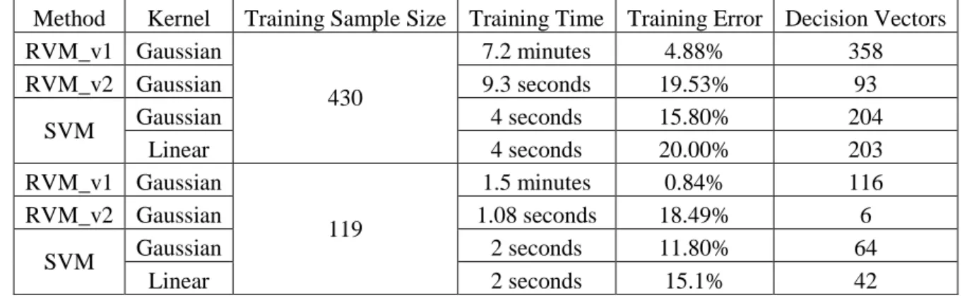
Table 2: Classification Accuracy during Training and Number of Decision Vectors for RVMs 26
and SVMs 27
Method Kernel Training Sample Size Training Time Training Error Decision Vectors RVM_v1 Gaussian 430 7.2 minutes 4.88% 358 RVM_v2 Gaussian 9.3 seconds 19.53% 93 SVM Gaussian 4 seconds 15.80% 204 Linear 4 seconds 20.00% 203 RVM_v1 Gaussian 119 1.5 minutes 0.84% 116 RVM_v2 Gaussian 1.08 seconds 18.49% 6 SVM Gaussian 2 seconds 11.80% 64 Linear 2 seconds 15.1% 42 28
As can be seen from Table 2, training for RVMs is slower than SVMs, something which 29
agrees with the results of other RVM classification works (13, 26). The delay in training for RVMs is 30
triggered by the iterated need for calculating and inverting the Hessian matrix and which leads to 31
more computational time, as sample size increases. The best classification is performed by the 32
RVM_v1 algorithm, with a large margin (of about 10%) to the next more successful algorithm which 33
is the SVM with a Gaussian kernel. However, it is noticeable that this successful rate of classification 34
by the RVM_v1 algorithm is due to the large number of decision vectors, which is about 1.5 to 2 35
times higher than the decision vectors used by RVM_v2 and SVM. The efficient RVM_v2 is about 36
4% less accurate than SVMs but the interesting fact is that it uses less than half of the decision vectors 37
utilised by SVMs to perform the training classification and in a non-critical time interval which can be 38
utilised in real-time (8 seconds). In the smaller sample size, it can also be seen that RVM_v2 uses 39
only 6 vectors to perform the classification, while the other two approaches require a much larger 1
number. Comparing training classification results between the small and the bigger sample size, it can 2
be seen that all three algorithms perform better on the small sample, which also agrees with the 3
literature (26, 27). It should be noted here that training time for SVMs is notably faster because of the 4
fact that SVMs are quite a popular classification algorithm and the corresponding toolboxes or other 5
software packages have undertaken a lot of attention in order to accelerate the algorithm’s outputs. 6
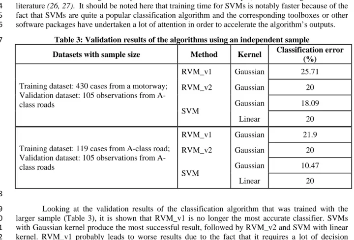
Table 3: Validation results of the algorithms using an independent sample 7
Datasets with sample size Method Kernel Classification error
(%)
Training dataset: 430 cases from a motorway; Validation dataset: 105 observations from
A-class roads RVM_v1 Gaussian 25.71 RVM_v2 Gaussian 20 SVM Gaussian 18.09 Linear 20
Training dataset: 119 cases from A-class road; Validation dataset: 105 observations from
A-class roads RVM_v1 Gaussian 21.9 RVM_v2 Gaussian 20 SVM Gaussian 10.47 Linear 20 8
Looking at the validation results of the classification algorithm that was trained with the 9
larger sample (Table 3), it is shown that RVM_v1 is no longer the most accurate classifier. SVMs 10
with Gaussian kernel produce the most successful result, followed by RVM_v2 and SVM with linear 11
kernel. RVM_v1 probably leads to worse results due to the fact that it requires a lot of decision 12
vectors and these classifier vectors cannot perform well when applied to an unknown independent 13
dataset. When the classifier was trained with a small sample and the algorithm was applied to a 14
relatively small sample, the results show that SVMs with Gaussian kernel outperform RVMs with a 15
classification error which is half of the classification error of both RVMs algorithms. 16
To further investigate the classification performance of the three algorithms2, the measures of 17
sensitivity and specificity were employed. For that purpose, four commonly employed terms (as 18
defined below) are employed. 19
• True Positive (TP): Dangerous (collision-prone) conditions (treal=1) correctly 20
identified as dangerous (tclassified=1) 21
• False Positive (FP): Dangerous (collision-prone) conditions (treal=1) 22
incorrectly identified as safe (tclassified=0) 23
• True Negative (TN): Safe traffic conditions (treal=0) correctly identified as safe 24
(tclassified=0) 25
• False Negative (FN): Safe traffic conditions (treal=0) incorrectly identified as 26
dangerous (tclassified=1) 27
28
By making use of the known formula for sensitivity and specificity (33), the performance of 29
these algorithms for the larger training dataset and the validation dataset are presented in Table 4: 30 𝑆𝑆𝑉𝑉𝑆𝑆𝑆𝑆𝑆𝑆𝑡𝑡𝑆𝑆𝑆𝑆𝑆𝑆𝑡𝑡𝑦𝑦=𝑇𝑇𝑀𝑀+𝐹𝐹𝑁𝑁𝑇𝑇𝑀𝑀 and 𝑆𝑆𝑆𝑆𝑉𝑉𝑐𝑐𝑆𝑆𝑓𝑓𝑆𝑆𝑐𝑐𝑆𝑆𝑡𝑡𝑦𝑦= 𝑇𝑇𝑁𝑁 𝑇𝑇𝑁𝑁+𝐹𝐹𝑀𝑀 (9) 31 2
SVM with linear kernel was excluded in Table 4 because it did not provide better results than the other algorithms
1
Table 4: Sensitivity and Specificity of RVMs and SVMs (N= 430+105=535) 2
Method Kernel TN FN TP FP Sensitivity (%) Specificity (%)
RVM_v1 Gaussian 419 9 68 39 88.4 91.5
RVM_v2 Gaussian 427 1 2 105 66.67 80.26
SVM Gaussian 417 11 31 76 73.8 84.6
3
It is noticeable from Table 4 that the RVM_v1 algorithm performs we in identifying the 4
traffic conditions that lead to a collision. RVM_v1 is the best classifier with 88.4% sensitivity and 5
91.5% specificity implying minimum Type I and Type II errors. The RVM_v2 algorithm 6
underperforms in terms of sensitivity and specificity among the two datasets. This is probably a result 7
of the greediness of the algorithm which converges fast but at the expense of a large number of false 8
positives. 9
The reason for these misclassification rates associated with all the algorithms, especially with 10
RVM may relate to the use of highly aggregated (i.e. 15-minute) traffic data, relatively small sample 11
size and the use of only two variables for representing traffic. In addition, the algorithm was primarily 12
trained with traffic data from a motorway (M1 J10 – J13) but validated with traffic data from A-class 13
roads. Traffic dynamics between these two classes of roads are quite different. 14
15
CONCLUSIONS 16
Machine learning approaches, especially support vector machines, have become a credible 17
solution for real-time collision prediction and traffic pattern recognition over the recent decades. Their 18
strengths lie in the use of a kernel function to control non-linearity and the efficient handling of 19
arbitrarily structured data. The performance of a SVM however largely relies on the kernel function 20
and the number of decision vectors that increases proportionately with the size of the training dataset. 21
The novelty of this work relates to the application of Relevance Vector Machines, a Bayesian 22
analogue to SVMs, for the task of classifying traffic conditions. RVMs have proven to be an efficient 23
classifier when applied to other pattern recognition tasks, but had not been applied in transport 24
studies. Classification was performed using highly aggregated 15-minute traffic measurements of 25
average speed and volume while a matched case-control structure was adopted to remove spatial 26
influence on the collision occurrence. Two different RVM classifiers were trained with a small (i.e. 27
119 collision and non-collision cases on an A-Road) and a relatively large training dataset (i.e. 430 28
collision and non-collision cases on a motorway) and were validated with an independent dataset of 29
105 collision and non-collision cases from a separate A-class road. In order to increase the 30
understanding on the classification differences between RVMs and SVMs, specificity and sensitivity 31
measures were calculated for each of the classification algorithms. 32
The advantage of RVM classification relates to the fact that the decision vectors it used to 33
classify new data are significantly fewer than the decision vectors used by SVMs. This may lead to 34
faster classification decisions which are crucial in real-time applications. Furthermore, the assignment 35
of a posterior probability to each classified instance makes RVMs more useful to experts and more 36
substantial than the non-probabilistic results of SVMs. However, attention should be given to the 37
training of the algorithm, so as to overcome misclassification errors and assure robustness with new 38
data. Classifying traffic conditions in order for the classification to be used in real-time collision 39
prediction is a promising direction for improving the efficiency and computational speed of current 40
collision prediction algorithms. RVMs with the small number of decision vectors they need in order to 41
classify conditions can prove helpful in this direction. On the other hand, improvements need to be 42
done in order for RVM classification to become more efficient. First of all, the incorporation of 43
disaggregated data should give a much clearer picture on the strengths of RVMs for real-time traffic 44
conditions classification. Furthermore, the inclusion of other traffic or network variables (e.g. traffic 45
density, vehicle compositions, variable speed limits) should be used to describe the collision-prone 1
conditions in a more realistic way. Lastly, training could take place with a large amount of data, so as 2
to more accurately describe traffic conditions and circumstantial precursors leading to traffic 3
accidents. 4
ACKNOWLEDGEMENT 5
This research was funded by a grant from the UK Engineering and Physical Sciences Research 6
Council (EPSRC) (Grant reference: EP/J011525/1). The authors take full responsibility for the content 7
of the paper and any errors or omissions. Research data for this paper are available on request from 8
Mohammed Quddus ([email protected]). 9 10 11 REFERENCES 12 13
1. Hummel, T., M. Kühn, J. Bende, and A. Lang. Advanced Driver Assistance Systems: An 14
investigation of their potential safety benefits based on an analysis of insurance claims in 15
Germany. Research report FS 03, German Insurance Association, 2011. 16
2. Thrun, S. Toward Robotic Cars. Communications of the ACM, Vol. 53, No. 4 (April), 2010, pp. 17
99–106. 18
3. Highways Agency, and Robert Goodwill. New generation of motorway opens on M25 - UK 19
Government Press release. https://www.gov.uk/government/news/new-generation-of-20
motorway-opens-on-m25, Accessed July 29t,2015 21
4. Lee, C., B. Hellinga, and F. Saccomanno. Real-time crash prediction model for application to 22
crash prevention in freeway traffic. In Transportation Research Board 82nd Annual Meeting, 23
Washington DC, United States, 2003.. 24
5. Hossain, M., and Y. Muromachi. A real-time crash prediction model for the ramp vicinities of 25
urban expressways. IATSS Research, Vol. 37, No. 1, Jul. 2013, pp. 68–79. 26
6. Abdel-aty, M., and A. Pande. The viability of real-time prediction and prevention of traffic 27
accidents. Efficient Transportation and Pavement, Taylor & Francis Group, pp 215-227, 2009.. 28
7. Abdel-Aty, M., A. Pande, L. Y. Hsia, and F. Abdalla. The Potential for Real-Time Traffic 29
Crash Prediction. ITE Journal on the web, 2005, pp. 69–75. 30
8. Ahmed, M. M., and M. a. Abdel-Aty. The Viability of Using Automatic Vehicle Identification 31
Data for Real-Time Crash Prediction. IEEE Transactions on Intelligent Transportation 32
Systems, Vol. 13, No. 2, Jun. 2012, pp. 459–468. 33
9. Hassan, H. M., and M. Abdel-Aty. Predicting reduced visibility related crashes on freeways 34
using real-time traffic flow data. Journal of safety research, Vol. 45, Jun. 2013, pp. 29–36. 35
10. Pande, A., and M. Abdel-Aty. Assessment of freeway traffic parameters leading to lane-36
change related collisions. Accident; analysis and prevention, Vol. 38, No. 5, Sep. 2006, pp. 37
936–48. 38
11. Hossain, M., and Y. Muromachi. A real-time crash prediction model for the ramp vicinities of 39
urban expressways. IATSS Research, Vol. 37, No. 1, Jul. 2013, pp. 68–79. 40
12. Yu, R., and M. Abdel-Aty. Multi-level Bayesian analyses for single- and multi-vehicle 41
freeway crashes. Accident; analysis and prevention, Vol. 58, Sep. 2013, pp. 97–105. 42
13. Tipping, M. Sparse Bayesian Learning and the Relevance Vector Machine. Journal of 43
Machine Learning Research, Vol. 1, 2001, pp. 211–244. 44
14. Vapnik, V. The nature of statistical learning theory. Springer-Verlag, New York, 1995. 45
15. Yuan, F., and R. L. Cheu. Incident detection using support vector machines. Transportation 46
Research Part C: Emerging Technologies, Vol. 11, No. 3-4, 2003, pp. 309–328. 47
16. Chen, S., W. Wang, and H. van Zuylen. Construct support vector machine ensemble to detect 48
traffic incident. Expert Systems with Applications, Vol. 36, No. 8, 2009, pp. 10976–10986. 49
17. Xiao, J., and Y. Liu. Traffic Incident Detection Using Multiple Kernel Support Vector 50
Machine. in Proceedings of the 2012 15th International IEEE Conference on Intelligent 51
Transportation Systems, 2012, pp. 1669-1673. 52
18. Ma, Y., M. Chowdhury, A. Sadek, and M. Jeihani. Real-time highway traffic condition 1
assessment framework using vehicleInfrastructure integration (VII) with artificial intelligence 2
(AI). IEEE Transactions on Intelligent Transportation Systems, Vol. 10, No. 4, 2009, pp. 615– 3
627. 4
19. Yu, R., G. Wang, J. Zheng, and H. Wang. Urban Road Traffic Condition Pattern Recognition 5
Based on Support Vector Machine. Journal of Transportation Systems Engineering and 6
Information Technology, Vol. 13, No. 1, 2013, pp. 130–136. 7
20. Li, X., D. Lord, Y. Zhang, and Y. Xie. Predicting motor vehicle crashes using Support Vector 8
Machine models. Accident Analysis and Prevention, Vol. 40, No. 4, 2008, pp. 1611–1618. 9
21. Yu, R., and M. Abdel-Aty. Utilizing support vector machine in real-time crash risk evaluation. 10
Accident; analysis and prevention, Vol. 51, Mar. 2013, pp. 252–259. 11
22. Wang, W., X. Qu, W. Wang, and P. Liu. Real-time freeway sideswipe crash prediction by 12
support vector machine. IET Intelligent Transport Systems, Vol. 7, No. 4, 2013, pp. 445–453. 13
23. Dong, N., H. Huang, and L. Zheng. Support vector machine in crash prediction at the level of 14
traf fi c analysis zones : Assessing the spatial proximity effects. Vol. 82, 2015, pp. 192–198. 15
24. Chen, S., S. R. Gunn, and C. J. Harris. The relevance vector machine technique for channel 16
equalization application. IEEE Transactions on Neural Networks, Vol. 12, No. 6, 2001, pp. 17
1529–1532. 18
25. Carin, L., and G. J. Dobeck. Relevance vector machine feature selection and classification for 19
underwater targets. Oceans 2003. Celebrating the Past ... Teaming Toward the Future (IEEE 20
Cat. No.03CH37492), Vol. 2, 2003, p. 933-957. 21
26. Demir, B., and S. Ertürk. Hyperspectral Image Classification Using Relevance Vector 22
Machines. 2007 IEEE International Geoscience and Remote Sensing Symposium, Vol. 4, No. 4, 23
2007, pp. 586–590. 24
27. Phillips, C. L., M. A. Bruno, P. Maquet, M. Boly, Q. Noirhomme, C. Schnakers, A. 25
Vanhaudenhuyse, M. Bonjean, R. Hustinx, G. Moonen, A. Luxen, and S. Laureys. “Relevance 26
vector machine” consciousness classifier applied to cerebral metabolism of vegetative and 27
locked-in patients. NeuroImage, Vol. 56, No. 2, 2011, pp. 797–808. 28
28. Wei, L., Y. Yang, R. M. Nishikawa, M. N. Wernick, and A. Edwards. Relevance vector 29
machine for automatic detection a of clustered microcalcifications. IEEE Transactions on 30
Medical Imaging, Vol. 24, No. 10, 2005, pp. 1278–1285. 31
29. Imprialou, M., M. Quddus, and D. Pitfield. Exploring the Role of Speed in Highway Crashes : 32
Pre-Crash-Condition-Based Multivariate Bayesian Modelling. In Transportation Research 33
Board 94th Annual Meeting, Washington DC, United States, 2015. 34
30. Michael E. Tipping. A Baseline Matlab Implementation of “ Sparse Bayesian ” Model 35
Estimation. Baseline, 2009. 36
31. Michael E. Tipping. An Efficient Matlab Implementation of the Sparse Bayesian Modelling 37
Algorithm (Version 2.0). 2009. 38
32. Tipping, M. E., and A. C. Faul. Fast Marginal Likelihood Maximisation for Sparse Bayesian 39
Models. Ninth International Workshop on Aritficial Intelligence and Statistics, No. x, 2003, pp. 40
1–13. 41
33. Powers, D. Evaluation : From Precision , Recall And F-Measure To ROC , Informedness , 42
Markedness & Correlation. Journal of Machine Learning Technologies, Vol. 2, No. 1, 2011, 43
pp. 37–63. 44