An In-depth Comparison of Subgraph Isomorphism
Algorithms in Graph Databases
Jinsoo Lee
∗School of Computer Science and Engineering Kyungpook National University, Korea
[email protected]
Wook-Shin Han
∗†School of Computer Science and Engineering Kyungpook National University, Korea
[email protected]
Romans Kasperovics
∗School of Computer Science and Engineering Kyungpook National University, Korea
[email protected]
Jeong-Hoon Lee
School of Computer Science and Engineering Kyungpook National University, Korea
[email protected]
ABSTRACT
Finding subgraph isomorphisms is an important problem in many applications which deal with data modeled as graphs. While this problem is NP-hard, in recent years, many algo-rithms have been proposed to solve it in a reasonable time for real datasets using different join orders, pruning rules, and auxiliary neighborhood information. However, since they have not been empirically compared one another in most research work, it is not clear whether the later work outper-forms the earlier work. Another problem is that reported comparisons were often done using the original authors’ bi-naries which were written in different programming envi-ronments. In this paper, we address these serious problems by re-implementing five state-of-the-art subgraph isomor-phism algorithms in a common code base and by comparing them using many real-world datasets and their query loads. Through our in-depth analysis of experimental results, we report surprising empirical findings.
1. INTRODUCTION
Many complex objects, such as chemical compounds, so-cial networks, and biological structures are modeled as graphs. Many real applications in bioinformatics, chemistry, and software engineering require efficient and effective manage-ment of graph structured data.
One of most important graph queries in graph databases is the subgraph isomorphism query. That is, given a queryq
and a data graphg, find all embeddings ofqing. This prob-lem belongs to NP-hard [10] and has many important ap-plications, such as searching chemical compound databases, ∗The first three authors contributed equally to this work. †Corresponding author
Permission to make digital or hard copies of all or part of this work for personal or classroom use is granted without fee provided that copies are not made or distributed for profit or commercial advantage and that copies bear this notice and the full citation on thefirst page. To copy otherwise, to republish, to post on servers or to redistribute to lists, requires prior specific permission and/or a fee. Articles from this volume were invited to present their results at The 39th International Conference on Very Large Data Bases, August 26th - 30th 2013, Riva del Garda, Trento, Italy.
Proceedings of the VLDB Endowment, Vol. 6, No. 2
Copyright 2012 VLDB Endowment 2150-8097/12/12...$10.00.
querying biological pathways, and finding protein complexes in protein interaction networks.
Ullmann [14] proposes the first practical algorithm for subgraph isomorphism search for graphs. It is a backtrack-ing algorithm which finds solutions by incrementbacktrack-ing partial solutions or abandoning them when it determines they can-not be completed. In recent years, many algorithms such as VF2 [2], QuickSI [11], GraphQL [5], GADDI [17], and SPath [18] have been proposed to enhance the Ullmann algorithm. These algorithms exploit different join orders, pruning rules, and auxiliary information to prune out false-positive candidates as early as possible, thereby increasing performance.
Figure 1 shows the reported comparisons of the state-of-the-art subgraph isomorphism algorithms. Here, a directed edge depicts reported superiority. For example, according to [18], SPath is superior to GraphQL. Note that, in [17], GADDI is compared with TALE [13] which finds only
ap-proximate embeddings. GraphQL SPath QuickSI GADDI Ullmann [2] VF2 [19] [12]
Figure 1: Comparisons of state-of-the-art graph iso-morphism algorithms.
We observe serious problems in the current practice of experiments for these algorithms: 1) It is difficult to com-pare each algorithm since they have not been described in a common framework; 2) They have not been compared em-pirically in most research work. Only four comparisons as depicted in Figure 1 were reported. Thus, it is not clear whether the later work outperforms the earlier work; 3) The reported comparisons were done by comparing the bi-nary executables provided by the original authors, ignoring a number of factors that heavily influence the performance (e.g., programming languages, implementer’s programming skills, main memory vs. disk, and buffer size, etc.).
In order to address these problems, we re-implement all representative subgraph isomorphism algorithms in a com-mon framework using C++. For this purpose, we use best-effort re-implementations based on the original papers and
on email communications with the original authors, since we were unable to acquire the source code of any technique except VF2 from its authors. However, since GraphQL is implemented in Java, we exploit a java bytecode ana-lyzer to fully understand the original implementation. We also perform extensive experiments using many real datasets and their query workload and provide an in-depth analy-sis. We note that a similar experience has been reported in iGraph [3], which compares only graph indexing tech-niques rather than the subgraph isomorphism algorithms themselves.
Our contributions can be summarized as follows.
• We clearly explain the differences of existing algorithms using a common framework in Section 3.
• We re-implement five state-of-the-art algorithms (VF2, QuickSI, GraphQL, GADDI, and SPath) in the com-mon code base.
• We fairly and empirically compare these algorithms using many real and synthetic datasets in Section 4. • We analyze experiments in depth in order to
under-stand why one algorithm outperforms another for spe-cific query and data graphs in Section 4
• We report surprising findings through our analysis: 1) QuickSI designed for handling small graphs often out-performs the more recent algorithms GraphQL, GADDI, and SPath which are designed for handling large graphs. 2) QuickSI, VF2, and GADDI fail to find embeddings in trees in a reasonable time, showing exponential be-havior. 3) GraphQL is the only method to process all query sets tested but shows slower performance than QuickSI in many query sets and datasets. 4) It should be noted that in this paper, unlike in [18], SPath is almost consistently slower than GraphQL. This is mainly because a) they are implemented in different programming languages, and b) the cost of reading signatures fromdisk is not taken into account. Note that SPath is implemented in C++, while GraphQL is implemented in Java. This strongly indicates that, unless both methods are implemented in a common framework, empirical comparisons would be useless. 5) We find that all existing algorithms have problems in their join order selections for some datasets, al-though GraphQL processes all queries we test in rea-sonable times. The blind computation of signatures of GraphQL regardless of queries and data sets in-curs significant performance overhead compared with QuickSI. This calls for new subgraph algorithms com-bining the strengths of both algorithms.
The remainder of this paper is organized as follows. Sec-tion 2 reviews the background informaSec-tion as well as exist-ing work on subgraph isomorphism. Section 3 presents the details of our implementations. Section 4 presents the re-sults of performance evaluation. Section 5 summarizes and concludes our paper.
2. BACKGROUND
2.1 Problem De
fi
nition
All datasets and query sets used in [2, 5, 11, 17, 18] are modeled asundirected labeled graphs. An undirected labeled graphgis defined as a triple (V, E, L) whereV is the set of vertices,E(⊆V×V) is the set of undirected edges, andLis a labeling function which maps a vertex or an edge to a set
of labels or a label, respectively. Without loss of generality, all subgraph isomorphism algorithms can be easily extended to handle graphs whose edges have a set of labels. Unless otherwise specified, we use symbolsq,g,u, andvto denote a query graph, a data graph, a query vertex, and a data vertex, respectively.
Given a query graph q = (V, E, L), a data graph g =
(V, E, L), a subgraph isomorphism (or an embedding) is
an injective function M : V → V such that (1) ∀u ∈ V,
L(u)⊆L(M(u)), and (2)∀(ui, uj)∈E, (M(ui),M(uj))∈
E, andL(ui, uj) =L(M(ui),M(uj)).
Problem Definition 1. [5, 14, 18]Given a query graphq
and a data graphg, the subgraph isomorphism problem is to
find all distinct embeddings ofq in g.
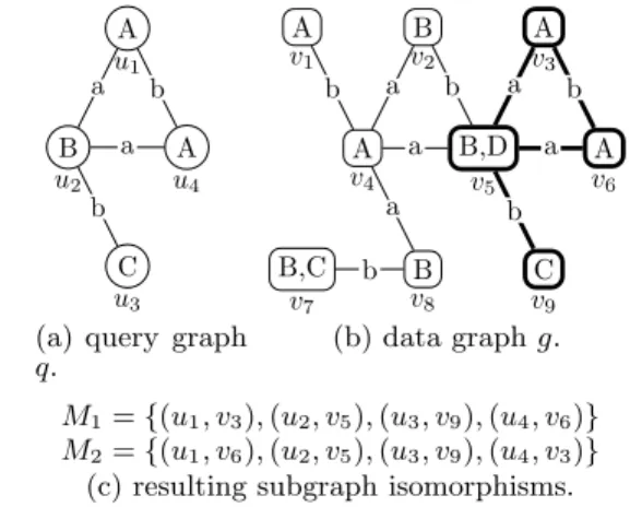
Figure 2 shows an example of query q and data graph
g. We have two embeddings M1 and M2 for this subgraph isomorphism query. A B C A a b b a u1 u2 u3 u4
(a) query graph
q. A B A A B,D A B,C B C b a b a b a a a b b v1 v2 v3 v4 v5 v6 v7 v8 v9 (b) data graphg. M1={(u1, v3),(u2, v5),(u3, v9),(u4, v6)} M2={(u1, v6),(u2, v5),(u3, v9),(u4, v3)} (c) resulting subgraph isomorphisms.
Figure 2: Example of query and data graphs.
In practice, we may stop the subgraph isomorphism search after the firstkembeddings are found. In [5, 18],kis set to 1000.
2.2 Basic Concepts
We explain the concept of the induced subgraph, the par-tial subgraph isomorphism, the adjacency set, and the k -neighborhood.
A graphqis aninduced subgraph of a graphqiff V(q)⊆ V(q), and E(q) contains only the edges present in q, i.e., E(q) = E(q)∩(V(q)×V(q)). Note that an induced sub-graphqofqcan be defined solely with its vertex set V(q). For example, the induced graph of the verticesv3, v5, v6, v9 is marked with bold lines in Figure 2.
Let g be an induced subgraph of g, and let M be a subgraph isomorphism from g to g. We call M apartial
solution when searching all subgraph isomorphisms fromg
togif V(g)⊂V(g) (as opposed to acomplete solutionsuch that V(g) = V(g)).
Theadjacency set of a vertexvof a graphg, denoted as
adj(v), is a set of vertices directly connected (adjacent) to
v. The k-neighborhood of a vertexvof a graphg, denoted as Nk(v), is a set of vertices ofgwhere for each vertexvin Nk(v), the shortest distance betweenvandvis less than or equal tok. That is, Nk(v) includesvitself.
Consider the vertex v4 in the data graph g from Fig-ure 2(b). The adjacency set adj(v4) is{v1, v2, v5, v8}. The 1-neighborhood N1(v4) is{v1, v2, v4, v5, v8}. The 2-neighborhood N2(v4) contains all vertices in the data graphg.
2.3 Related Work
We can classify existing algorithms into two categories depending on whether or not they use exact search: (1)exact
subgraph matching and (2)approximatesubgraph matching. Each matching has its own important target applications.
Exact subgraph matching algorithms can also be classi-fied into two subcategories depending on the usage of graph indexing techniques. The first subcategory includes Graph-Grep [12], gIndex [16], FG-Index [1], Tree+Δ [19], gCode [20], SwiftIndex [11], and C-Tree [4]. These indexing al-gorithms are based on a two-step filter-and-refine strategy where the filtering step uses graph indexes to minimize the number of candidate graphs, and the refinement step checks if there exists one subgraph isomorphism for each candi-date. The second subcategory includes Ullmann [14], VF2 [2], QuickSI [11], GraphQL [5], GADDI [17], and SPath [18]. These algorithms findallembeddings for a given query graph and a data graph. We will detail each algorithm in the following section. We note that Ullmann, VF2, and QuickSI have been originally designed for handling small
graphs while GraphQL, GADDI, and SPath have been orig-inally designed for handlinglarge graphs.
Approximate subgraph matching algorithms find approx-imate embeddings with their own similarity measures. Rep-resentative algorithms in this area include TALE [13], SIGMA [9], and Ness [6].
3. IMPLEMENTATION
In this section, we describe how we implement the five state-of-the-art algorithms in a common framework. For this purpose, we introduce a generic subgraph isomorphism algorithm so that each algorithm can be implemented by extending this generic algorithm according to its specifics.
3.1 Generic Subgraph Isomorphism Algorithm
The generic subgraph isomorphism algorithm is imple-mented as a backtracking algorithm [7] which finds solutions by incrementing partial solutions or abandoning them when it determines they cannot be completed.
Algorithm 1 shows a generic subgraph isomorphism algo-rithm,GenericQueryProc. Its inputs are a query graph q and a data graph g, and its output is a set of subgraph isomorphisms (or embeddings) ofqin g. Here, to represent an embedding, we use a list M of pairs of a query vertex and a corresponding data vertex.
For each vertexuinq,GenericQueryProcfirst invokes
FilterCandidatesto find a set of candidate verticesC(u)
(⊆ V(g)) such that L(u) ⊆ L(v) (Line 3). Note that we place logical expressions in double square brackets to show
thenecessary post-conditions for each subroutine. If C(u)
is empty, we can safely exit, making early termination pos-sible (Line 5). After that, GenericQueryProcinvokes a
recursive subroutine, SubgraphSearch, to find mapping
pairs of a query vertex and matching data vertices at a time (Line 8). Note thatSubgraphSearch of SPath matches
one query path at a time for each recursive call.
SubgraphSearchSubroutine
SubgraphSearchtakes as parameters a query graphq, a
data graph g, and a partial embeddingM and reports all embeddings ofqing.
The recursion stops when the algorithm finds the complete solution (i.e., when|M|=|V(q)|) (Line 1). Otherwise, the
algorithm callsNextQueryVertexto select a query vertex u∈V(q) which is not yet matched (Line 4). After that, it callsRefineCandidatesto obtain a refined candidate
ver-tex set CR fromC(u) by using algorithm-specific pruning rules (Line 5). Next, for each candidate data vertexv∈CR such thatvis not matched yet, theIsJoinablesubroutine
checks whether the edges between u and already matched query vertices ofqhave corresponding edges betweenvand already matched data vertices ofg(Line 7). Ifvis qualified, it is matched to u, and SubgraphSearch updates status
information by calling UpdateState(Line 9), and the
al-gorithm proceeds to match the remaining query vertices of
qby recursively callingSubgraphSearch(Line 10). Next,
all changes done by UpdateStateare restored by calling
RestoreState(Line 11). The algorithm terminates when
all possible embeddings are found.
Algorithm 1GenericQueryProc
Input: query graphq Input: data graphg
Output: all subgraph isomorphisms ofqing 1: M:=∅; 2: for eachu∈V(q)do 3: C(u) :=FilterCandidates(q, g, u, . . .); [[∀v∈C(u)((v∈V(g))∧(L(u)⊆L(v))) ]] 4: ifC(u) =∅then 5: return; 6: end if 7: end for 8: SubgraphSearch(q, g, M, . . .); SubroutineSubgraphSearch(q, g, M, . . .) 1: if|M|=|V(q)|then 2: reportM; 3: else 4: u:=NextQueryVertex(. . .); [[u∈V(q)∧ ∀(u, v)∈M(u=u) ]] 5: CR:=RefineCandidates(M, u, C(u), . . .); [[CR⊆C(u) ]]
6: for eachv∈CRsuch thatvis not yet matcheddo
7: ifIsJoinable(q, g, M, u, v, . . .)then 8: [[∀(u, v)∈M((u, u)∈E(q) =⇒ (v, v)∈E(g)∧L(u, u) = L(v, v)) ]] 9: UpdateState(M, u, v, . . .); [[ (u, v)∈M]] 10: SubgraphSearch(q, g, M, . . .); 11: RestoreState(M, u, v, . . .); [[ (u, v)∈/M]] 12: end if 13: end for 14: end if
The SPath algorithm grows partial solutions with one path at a time rather than a vertex at a time. Thus, al-though our generic recursive algorithm accommodates the characteristics of SPath, we will explain SPath separately in Section 3.7 for ease of understanding.
Common Graph Storage
Depending on the size of a data graph, we store the graph as a tuple in a heap file or a large object in a BLOB file as in iGraph. We also use a B+-tree to efficiently find a data graph using a graph ID.
For each subgraph isomorphism algorithm, we tune the disk representation of a data graph in order to support fast retrieval and construction of its main memory data tures. In subsequent subsections, we describe data struc-tures for each method.
3.2 Ullmann Algorithm
FilterCandidates: FilterCandidates returns a set of
data graph vertices with a matching labelu.
NextQueryVertex:NextQueryVertexreturns one
ver-tex at a time from the vertices in the order they appear in the input. It is clear that the performance of the Ullmann algorithm highly depends on the input order of the query vertices. We will describe this issue in detail when we de-scribe theNextQueryVertexfunction of VF2.
RefineCandidates:RefineCandidatesprunes out all
can-didate verticesv∈C(u) that have a smaller degree thanu.
IsJoinable:IsJoinableiterates throughalladjacent query
vertices of u. If the adjacent query vertex u is already matched, i.e., (u,v) ∈M, then it checks whether there is a corresponding edge (v,v) in the data graph. Note that, since IsJoinable is called in a most inner loop, we must
carefully design this function. If there is no edge between
uand already matched query vertices, we can optimize this process by skipping this checking process. Such optimiza-tion will be explained inIsJoinableof QuickSI.
UpdateState, RestoreState: UpdateStateappends a
pair (u, v) toMwhileRestoreStaterestoresM by
remov-ing the pair (u, v) fromM.
In the following algorithms, we describe only the subrou-tines which are different from those in Ullmann.
3.3 VF2 Algorithm
NextQueryVertex: Unlike Ullmann, VF2 starts with the
first vertex and selects a vertexconnected from the already matched query vertices. Note that the original VF2 algo-rithm does not define any order in which query vertices are selected.
RefineCandidates: VF2 uses the following three pruning
rules to prune out data vertex candidates: (1) Prune out any vertex v in C(u) such that v is not connected from already matched data vertices; (2) LetMq andMg be a set of matched query vertices and a set of matched data vertices, respectively. Let Cq and Cg be a set of adjacent and not-yet-matched query vertices connected fromMq and a set of adjacent and not-yet-matched data vertices connected from
Mg, respectively. Let adj(u) be a set of adjacent vertices to a vertexu. Then, prune out any vertexvinC(u) such that |Cq∩adj(u)|>|Cg∩adj(v)|; (3) prune out any vertexvin
C(u) such that|adj(u)\Cq\Mq|>|adj(v)\Cg\Mg|. For example, consider again the query graph q and the data graphgfrom Figure 2. Suppose that the current par-tial solution M = {(u1, v4)} and that u2 is the next ver-tex returned byNextQueryVertexwithC(u2) ={v2,v5, v7, v8}. Then, Mq = {u1}, Mg = {v4}, Cq = {u2, u4},
Cg = {v1, v2, v5, v8}. The RefineCandidatessubroutine
prunes out v7 using the pruning rule (1), because v7 is not connected to any vertex in Mg. The subroutine also prunes outv8 fromC(u2) using the pruning rule (2), since adj(u2)∩Cq={u4}and adj(v8)∩Cg={}. The subroutine prunes out v2 fromC(u2) using the pruning rule (3) since adj(u2)\Cq\Mq={u3}and adj(v2)\Cg\Mg ={}.
Improvements
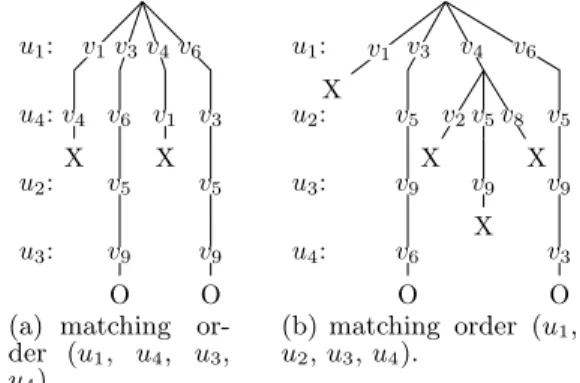
We note that the matching order driven by NextQueryVer-texsignificantly impacts the query performance by reducing
the size of the recursive call tree. For instance, consider the query and data graphs from Figure 2. If we match query vertices in order (u1, u2, u3, u4), SubgraphSearch of the
generic algorithm is called 14 times (Figure 3(b)). However, if we match query vertices in order (u1, u4, u2, u3),
Sub-graphSearch is called 12 times (see Figure 3(a)). Note
that in both cases, at least eight recursive calls are neces-sary to output two complete solutions.
u3: u2: u4: u1: X v4 v1 O v9 v5 v6 v3 X v1 v4 O v9 v5 v3 v6
(a) matching or-der (u1, u4, u3, u4). u4: u3: u2: u1: X v1 O v6 v9 v5 v3 X v2 X v9 v5 X v8 v4 O v3 v9 v5 v6 (b) matching order (u1, u2,u3,u4).
Figure 3: Recursion trees using the generic sub-graph isomorphism algorithm for the query and data graphs in Figure 2.
The original VF2 version used in iGraph uses a reorder-ing technique which sortsquery vertices by the frequency of the query vertex label and then feeds these reordered query vertices as input to VF2. This technique could be effective when the reordered vertex sequence is similar to the one or-dered by the frequency of the data vertex label. We also optimize the original VF2 version in several ways: 1) On comparing labels of two vertices, we directly compare the label IDs (i.e., integer comparison) of those vertices instead of calling expensive virtual function calls. 2) By exploiting the inverse vertex label list, we accelerate the search per-formance of finding vertices having a given vertex label. 3) When returning from each recursive call,CqandCgmust be restored. By maintaining additional stacks, this process can also be accelerated efficiently. By putting these optimiza-tions including the reordering technique all together, our VF2 version outperforms the original by up to 29.86 times.
Disk Representation
VF2 represents a graph using three structures: 1)vertex
la-bel list that allows access to the ordered vertex label list of
a vertex by a given ID (see Figure 4(a)); 2) inverse vertex
label list that allows access to the ordered vertex ID list by
a given vertex label (see Figure 4(b)); and 3)adjacency lists
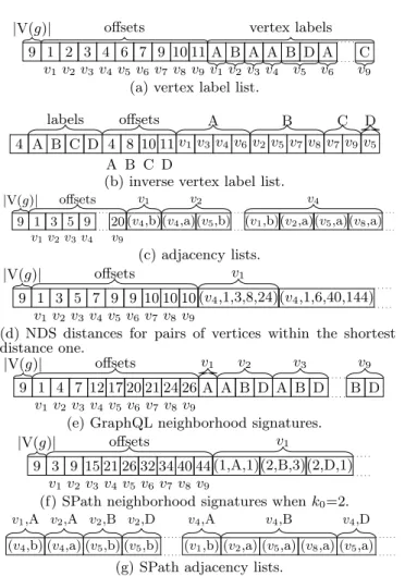
(see Figure 4(c)) of each vertex which store adjacency infor-mation, i.e., a list of pairs (vertex ID, edge label) ordered by the vertex ID. Note that we materialize the inverse vertex label list in the graph database for speedup, although it can be constructed from the vertex label list.
3.4 QuickSI Algorithm
NextQueryVertex: QuickSI tries to access vertices
hav-ing infrequent vertex labels and infrequent, adjacent edge labels as early as possible. Specifically, instead of using la-bel frequency information from a query graph as in VF2, QuickSI pre-processes data graphs to compute the frequen-cies of vertex labels and the frequenfrequen-cies of a triple (source vertex label, edge label, target vertex label). By using the computed edge label frequencies, we assign a weight to each query edge and obtain a minimum spanning tree using a modified Prim algorithm. QuickSI creates a sequence by using the order in which the vertices are inserted into the
9 |V(g)| 1 v1 2 v2 3 v3 4 v4 6 v5 7 v6 9 v7 10 v8 11 v9 offsets A B A A B D A C vertex labels v1v2v3v4 v5 v6 v9 (a) vertex label list.
4 A B C D labels 4 8 10 11 A B C D offsets v1v3v4v6v2v5v7v8v7v9v5 A B C D
(b) inverse vertex label list. 9 |V(g)| 1 v1 3 v2 5 v3 9 v4 20 v9 offsets
(v4,b)(v4,a)(v5,b) (v1,b)(v2,a)(v5,a)(v8,a)
v1 v2 v4 (c) adjacency lists. 9 |V(g)| 1 v1 3 v2 5 v3 7 v4 9 v5 9 v6 10 v7 10 v8 10 v9 offsets (v4,1,3,8,24)(v4,1,6,40,144) v1
(d) NDS distances for pairs of vertices within the shortest distance one. 9 |V(g)| 1 v1 4 v2 7 v3 12 v4 17 v5 20 v6 21 v7 24 v8 26 v9 offsets A A B D A B D B D v1 v2 v3 v9
(e) GraphQL neighborhood signatures. 9 |V(g)| 3 v1 9 v2 15 v3 21 v4 26 v5 32 v6 34 v7 40 v8 44 v9 offsets (1,A,1)(2,B,3)(2,D,1) v1
(f) SPath neighborhood signatures whenk0=2.
(v4,b) (v4,a) (v5,b) (v5,b) (v1,b) (v2,a) (v5,a) (v8,a) (v5,a) v1,A v2,A v2,B v2,D v4,A v4,B v4,D
(g) SPath adjacency lists.
Figure 4: Disk representation of the data graph from Figure 2.
minimum spanning tree. When the algorithm selects a start-ing edge (u1,u2), the algorithm uses u1 as the first vertex in the sequence if the vertex label frequency ofu1 is lower than that ofu2. Otherwise, u2 is used as the first vertex. For detailed explanation, we refer readers to [11].
RefineCandidates: For the first query vertexu, QuickSI
does not refine u. For the subsequent vertices u returned
byNextQueryVertex, letupar be the parent vertex ofu
in the minimum spanning tree andvbe the matching data vertex ofupar. Then, QuickSI prunes outvinC(u), if there is no edge betweenvandv.
IsJoinable: UnlikeIsJoinable of Ullmann which blindly
iterates throughalladjacent query vertices ofu,IsJoinable
of QuickSI iterates through adjacent and already matched query vertices ofu.
Although this important property is not elaborated in [11], our empirical analysis shows that this mechanism con-tributes to speedups of QuickSI, making the invocation cost of theSubgraphSearch of QuickSI the lowest among all
five algorithms.
Disk Representation
QuickSI stores a graph in the same format as the VF2 algo-rithm. In addition, QuickSI uses two B+-trees, one B+-tree for storing all distinct vertex labels along with their fre-quencies and the other for storing all distinct triples (source vertex label, edge label, target vertex label) along with their frequencies.
3.5 GADDI Algorithm
Before explaining each subroutine specific to GADDI, we first need to understand the concept of theneighboring
dis-criminating substructure (NDS) distance.
The NDS distance between v1 and v2 using a subgraph
P, denoted as ΔNDS(v1, v2, P), is defined as the number of embeddings ofP in an induced subgraph of Nk(v1)∩Nk(v2). Noth thatkis a given parameter of GADDI.
Figure 5 displays the data graph g from Figure 2 with the induced subgraph of N2(v1)∩N2(v4) drawn with thicker lines. For the substructures P1, P2, and P3 shown in the same figure, the NDS distances are calculated as follows: ΔNDS(v1, v4, P1) = 3; ΔNDS(v1, v4, P2) = 8; and ΔNDS(v1, v4, P3) = 24. A B A A B,D A B,C B C b a b a b a a a b b v1 v2 v3 v4 v5 v6 v7 v8 v9 P1 P2 P3 ΔNDS(v1, v4, P1) = 3, ΔNDS(v1, v4, P2) = 8, ΔNDS(v1, v4, P3) = 24
Figure 5: The NDS distances between v1 and v4
whenk = 2.
Now, we explain how GADDI selects substructures for calculating NDS distances. For this purpose, GADDI sam-ples 100 pairs of vertices from the data graph, and for each pair (v1,v2), we construct an induced unlabeled graph1 of Nk(v1)Nk(v2). For those induced graphs, [17] suggests selecting top ten frequent subgraphs using a frequent sub-graph mining algorithm such as gSpan [15]. We construct a matrixLwhere each row corresponds to an induced graphg, and each column corresponds to a subgraph selectedP, and each entry inLcorresponds to the number of embeddings of
P in g. We select the three columns (i.e., subgraphs) that have the largest numbers of distinct values as substructures.
NextQueryVertex: GADDI first selects a query vertex
appearing first in the input and then performs a depth-first search to find next query vertices.
RefineCandidates: RefineCandidates of the GADDI
algorithm prunes out v in C(u), if, for each query vertex
u ∈ Nk(u), there is no data vertex v ∈ Nk(v) satisfying the following three conditions: 1) L(u) ⊆ L(v); 2) for each Pi in a given set of substructures, ΔNDS(u, u, Pi) ≤ ΔNDS(v, v, Pi); and 3) the shortest distance betweenuand
uis greater than or equal to the shortest distance between
v andv.
UpdateState,RestoreState: GADDI uses an additional
pruning technique that reduces the candidate sets of all query vertices. For each data vertex v in Nk(v), if there does not exist a query vertex u in Nk(u) satisfying the three conditions used inRefineCandidates, we can prune v from all the current candidate sets exceptC(u). There-fore, UpdateStateidentifies those prunable data vertices
and additionally removes them from allC(ui)s exceptC(u) (1≤i≤ |V(q)|), andRestoreStateadditionally restores
the removed vertices.
1We have communicated with one of the original authors to learn how to construct such induced graphs.
Improvements
We use the reordering technique which is used in the im-proved VF2 version to reduce the size of the recursive call tree ofSubgraphSearch.
According to [17], subgraphs selected for computing NDS distances are connected, unlabeled graphs having three or four edges. Thus, there are only eight different connected graphs having three or four edges. By exploiting this impor-tant fact, we can safely skip the expensive frequent subgraph mining.
Disk Representation
GADDI stores a graph in the same representation as it does for the VF2 algorithm. In addition, for each pair of data vertices of a graph, we store the precomputed NDS and the shortest distances along with the graph. Specifically, for each pair (vi, vj) of vertices (i < j) within a given shortest distance, we store an entry storing the shortest distance and three NDS distances. These entries are ordered by the IDs of the first and the second vertices, and we use binary search to locate the distances between the given pair of vertices. Fig-ure 4(d) shows a fragment of the disk representation of the data graphg in Figure 2 storing the precomputed shortest distance and three NDS distances for the pairs of vertices within the distance of one. In this fragment,v1 has just one vertexv4within distance one fromv1, and the corresponding entry stores the NDS distances from Figure 5.
3.6 GraphQL Algorithm
FilterCandidates: The GraphQL algorithm uses two
ad-ditional pruning rules to reduce the size of the candidate sets: 1) neighborhood signature based pruning and 2) the pseudo subgraph isomorphism test based pruning.
We first explain the concept of theGraphQL neighborhood signatureof a vertexv, denoted as sigGraphQL(v). sigGraphQL(v) is a multiset of labels of adj(v). For example, sigGraphQL(u2) in Figure 2 is{A, A, C}, and sigGraphQL(v2) is{A, B, D}.
The neighborhood signature based pruning prunes out a candidate vertex v if sigGraphQL(u) sigGraphQL(v). For example, assume thatuisu2(Line 3 of Algorithm 1). Then,
v2 is pruned since sigGraphQL(u2)sigGraphQL(v2). Now, we explain the concept of the pseudo isomorphism test, which is an iterative algorithm using the depthdas a parameter. At first iteration, we obtain two breadth first search treesTuandTvforuandvrespectively, where their depth is 1(i.e.,d= 1). Then, we can prune outvifTuis not contained inTv. We can iterate this process by increasing
dby one untild=r, wherer is called therefinement level. For detailed explanation, we refer readers to [5].
NextQueryVertex: The GraphQL algorithm finds next
query vertices by using a greedy strategy similar to the heuristic-based join order optimization based on the cardi-nality of intermediate joined results. NextQueryVertex
of GraphQL first selects a query vertex u which has the smallest candidate set size|C(u)|. In the subsequent calls,
NextQueryVertexreturns a query vertexu that is
con-nected already matched query vertices and that makes the smallest size of intermediate results.
Improvements
For graphs having labeled edges, we extend GraphQL neigh-borhood signature ofvwith labels of the adjacent edges to
v to improve pruning power. For instance, sigGraphQL(v2) from Figure 2 becomes{(a,A), (b,B), (b,D)}.
Disk Representation
GraphQL stores a graph using an inverse vertex label list (see Figure 4(b)), an adjacency list(Figure 4(c)), and a GraphQL neighborhood signature (Figure 4(e)). GraphQL does not use the vertex label list, since it can construct candidate vertex lists during the neighborhood signature based prun-ing. Note that GraphQL materializes GraphQL neighbor-hood signatures of all vertices for a data graph, which is more efficient than constructing such signatures on the fly during query processing. Figure 4(e) illustrates the disk rep-resentation of GraphQL signatures of the data graph from Figure 2.
3.7 SPath Algorithm
The SPath algorithm also uses theGenericQueryProc,
though it invokes a differentSubgraphSearchin order to
match a querypathrather than a query vertex per recursive call. Thus, it may minimize the depth of the recursion tree by matching a path per call [18]. However, as we will see in our experiments, the selection order of paths significantly impacts the query performance, and the selection order of SPath is far from optimal for most data sets.
FilterCandidates: Similar to the GraphQL algorithm,
SPath uses neighborhood signatures to minimize candidate sets. However, it attempts to exploit more neighborhood information. The SPath neighborhood signature of a given vertexu, denoted as sigSPath(u), is a set of triples where each triple (d, l, c) is constructed from the vertices in Nk0(u). The
triple (d, l, c) represents the fact that there arecvertices in Nk0(u) containing the labellsuch that the shortest distance fromuis d. Here, k0 is called the neighborhood scope. For instance, if k0 = 1, the signature of vertex v7 in Figure 2 is sigSPath(v7) ={(1, B,1)}. Ifk0= 2, the signature of the same vertexv7 is sigSPath(v7) ={(1, B,1), (2, A,1)}.
Now, we explain how to use the SPath neighborhood sig-nature. We first define a function Sl
d(v) to represent the containment relationship between two SPath neighborhood signatures. If there exists a triple (d, l, c) in sigSPath(v),
Sl
d(v) =c. Otherwise,Sdl(v) = 0. Next, we define a rule for pruning data vertices using the SPath neighborhood signa-ture. For the given signatures sigSPath(u) and sigSPath(v) of query vertexuand data vertexv, we can prune out the data vertex vin C(u), if it does not satisfy the following condi-tion: for allk ≤k0 and all possible labels lin sigSPath(u),
k
i=1Sil(u) ≤
k
i=1Sil(v). For example, assume that u is
u3 (Line 3 of Algorithm 1) and that k0 = 2. Here, the sig-nature of u3 is ((1, B,1),(2, A,2)). We can prunev7, since
2
i=1SiA(u3)(= 2)>
2
i=1SAi(v7)(= 1).
Unlike [18] suggesting a large neighborhood scope (k0 = 4), we observe that, if we increase the neighborhood scope of SPath, the performance can decrease. This phenomenon is explained as follows. A larger neighborhood scope in-creases filtering power, but also inin-creases the size of SPath neighborhood signature and the filtering time. The optimal neighborhood scope, which is difficult to choose, lies in a balance between filtering power and filtering time.
The following subroutine showsSubgraphSearchof SPath.
Note that the neighborhood scopek0is used as an additional parameter in order to limit the radius of the SPath neigh-borhood signature of a vertex.
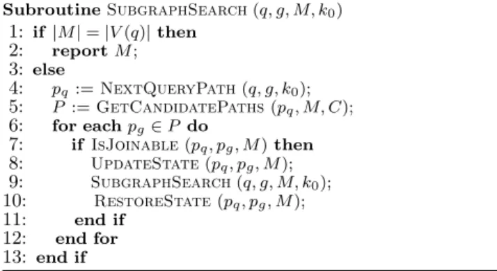
The subroutine stops this recursion when the algorithm finds the complete solution (i.e., when|M|=|V(q)|) (Line 1). Otherwise, the subroutine callsNextQueryPathto
se-lect a next querypath pq whose length is shorter than or equal tok0, and whose vertices except the first vertex are not yet matched. (Line 4). After that, it calls
GetCan-didatePathsto obtain all data paths matching the query
pathpq in the data graphg(Line 5). Next, for each candi-date data pathpg ∈P, theIsJoinable subroutine checks
whether the edges between the vertices in the pq and al-ready matched query vertices ofqhave corresponding edges between the vertices in the pg and already matched data vertices of g (Line 7). Note that the first vertex of pq is already matched, so all the resulting candidate data paths should start from the matched data vertex. Ifpg is quali-fied, it is matched topq, andSubgraphSearchupdates the
partial solutionM by calling UpdateState(Line 8), and
the algorithm proceeds to match the remaining query paths ofq by recursively callingSubgraphSearch(Line 9).
SubroutineSubgraphSearch(q, g, M, k0) 1: if|M|=|V(q)|then 2: reportM; 3: else 4: pq:=NextQueryPath(q, g, k0); 5: P :=GetCandidatePaths(pq, M, C); 6: for eachpg∈P do 7: ifIsJoinable(pq, pg, M)then 8: UpdateState(pq, pg, M); 9: SubgraphSearch(q, g, M, k0); 10: RestoreState(pq, pg, M); 11: end if 12: end for 13: end if
Now, we explain the subroutine NextQueryPath
fur-ther, which is most important in query performance of SPath.
NextQueryPath: The SPath algorithm first selects a query
vertexuwhich has the smallest candidate set size|C(u)|. In the subsequent call, SPath returns the most selective path which starts from an already matched query vertex. Here, the selectivity functionsel(p) for a given pathpis calculated as 2|V(p)|
u∈V(p)|C(u)|, where V(p) denotes all vertices in a path p. Note that the denominator represents the join cardinality of the candidate sets for all query vertices in p. However, this overestimate leads to significant errors in estimating the join cardinality. Thus, in many query and datasets, SPath is bound to choose a suboptimal join order.
Disk Representation
Like the GraphQL algorithm, SPath stores only the inverse vertex label list for accessing vertices by label and does not store the vertex label list, which is constructed in memory from the inverse vertex label listduring the SPath neighbor-hood signature based pruning. Each SPath neighborneighbor-hood signature for the data vertexvi is stored as a list of triples (d, l, c) ordered bydandl(Fig. 4(f)). As a distinction from all other methods, SPath adjacency lists are grouped by la-bels of target vertices. For example, in Fig. 4(g), the ad-jacency list of the vertex v4 is split into three sublists: 1) the adjacent vertices with label A ((v1, b)), 2) the adjacent vertices with label B ((v2, a),(v5, a),(v8, a)), and 3) the ad-jacent vertices with label D ((v5, a)).
4. EXPERIMENTS
In this section, we evaluate the performance of the five representative subgraph isomorphism algorithms VF2 [2], QuickSI [11] (in short, QSI), GraphQL [5] (in short, GQL), GADDI [17] (in short, GAD), and SPath [18] (in short,
SPA). We use best-effort reimplementations based on the original papers and on email communications with the orig-inal authors. As for GraphQL, we re-implement and opti-mize it in C++ by analyzing the original implementation using a java bytecode analyzer.
Datasets: We use four real datasets referred to here as AIDS, NASA, Yeast, and Human. The AIDS dataset was used in [11]. The Yeast dataset was used in [5, 18]. The NASA dataset was produced from a popular XML dataset [8] used in the XML research field. Since the Human dataset used in [17] could not be obtained from the original authors, we re-created it using the same process described in [17], which is straightforward. We also experimented with the synthetic datasets used in [5, 17]. However, there were no significant differences in overall performance trends of the algorithms, and thus, we omit them to save space.
Note that these datasets have different characteristics. The AIDS dataset contains a set ofsparsegraphs where the average graph size is small (= 27.4 in terms of the number of edges), and the number of unique labels is small (=51). The NASA dataset contains a set oftreeswhere the average tree size is 32.2, and the number of unique labels is much larger (=117,302) than AIDS. The Yeast dataset contains only one large graph having 3112 vertices and 12519 edges. A ver-tex corresponds to a protein, and an edge corresponds to an interaction between two proteins. Since one protein can ap-pear in several cellular components and biological processes, a vertex can have multiple labels. This graph isdenserthan graphs in AIDS and NASA. The Human dataset contains a large graph modeling a protein interaction network of 4675 proteins and 86282 interactions, which is larger and denser than Yeast. This graph has a fewer number of labels and a larger average degree than Yeast. Table 1 summarizes the properties of the four datasets.
Table 1: Summary of the real-world datasets.
Dataset AIDS NASA Yeast Human
# of graphs 10000 36790 1 1 # of vertices 2∼214 2∼889 3112 4675 # of edges 1∼217 1∼888 12519 86282 Avg. degree 1.95 1 8.05 36.82 Max. degree 11 245 168 771 # of distinct v. labels 51 117302 184 90 # of distinct e. labels 4 0 0 0
Avg. # of labels per vertex
1 1 7.55 4.63
Query sets: For AIDS, we use the existing query sets which are currently downloadable together with the iGraph frame-work2. There are six query sets. Each query set contains 1000 query graphs of the same size in terms of the number of edges. The query sizes are 4, 8, 12, 16, 20, and 24 edges. To generate queries of size 24, we randomly select connected subgraphs of size 24 from data graphs. We then generate the other query sets so that the following containment relation-ship is satisfied. That is, a small size query graph qof size
sis constructed from a large size query graphq of sizes+ 4 by removing edges untilqis still connected and contains
s edges. For the other datasets, we generate query sets by using this query generation process. In addition, we use two types of query sets for Yeast and Human which were used in [5]. These query sets were generated with a tool provided 2http://www.igraph.or.kr/
by the GraphQL authors and do not satisfy the containment relationship.
Suppose that a large query graph q is a supergraph of a small graphq. Then, the number of embeddings for qis typically smaller than or equal to the number of embeddings for q. Thus, the performance of a good subgraph isomor-phism algorithm would decrease as we increase the query size. In contrast, the search space for a graph q exponen-tially increases as we increase the query size. If a queryqhas
nvertices,u1,u2,· · ·,un, then the size of its search space becomes |C(u1)|×|C(u2)|×· · · ×|C(un)|. Thus, the perfor-mance of a good subgraph isomorphism algorithm is likely to decrease as we increase the query size by exploiting pow-erful pruning rules and optimal join orders.
Setup: For all experiments, we use a PC with Intel Xeon Quad Core 2.27GHz , 8 GB of main memory, and 1 TB 7200 RPM hard disk, running Windows Vista. We imple-ment all algorithms in the iGraph framework using C++ and compile them using Microsoft Visual-C++ compiler. We run all algorithms with best possible parameter values for each dataset. We stop subgraph isomorphism search after the first 1000 subgraph isomorphisms are found, as it was done in [5, 18]. The size of the database buffer is set to 500 MB, which allows the once read data from the database to be kept in main memory.
We use the number of I/Os and the elapsed time as the performance metrics for database construction. We use the average elapsed time and the average number of
Subgraph-Searchcalls (# of recursive calls) as the performance
met-rics for query execution. Specifically, if there is more than one data graph in a database, the elapsed time for a query means the accumulated elapsed time for processing all data graphs for that query. Thus, we average the total elapsed times for all queries to calculate the average elapsed time. Note that each algorithm has the significantly different cost
of aSubgraphSearchcall.
We divide our experimental section into four parts for each dataset and give more details on each dataset in the corresponding subsections.
4.1 AIDS Dataset
4.1.1 Database Construction
Table 2 shows the database sizes and database building times for all five algorithms using the AIDS dataset. Note that the number of read I/Os for all algorithms is 588. SPath was run with the best neighborhood scope k0 = 2. The GADDI algorithm was run with the shortest distanced= 1 and the neighborhood scope k0 = 2. Setting d = 1 and
k0= 2 produced the best performance results as in [17]. The VF2 database has the smallest disk space, and its building time is the fastest, since the VF2 algorithm does not use any auxiliary information. QuickSI has the same disk representation as VF2 along with two additional B+-trees to store the frequencies of 51 unique vertex labels and 240 unique edge features. However, the space of the frequency information of QuickSI for the AIDS dataset is negligible. Thus, the database sizes of both algorithms are almost the same. However, in QuickSI, for each data graph, we first count unique vertex labels and unique edge features and update the frequencies in the corresponding B+-trees, re-sulting in 33582 + 60214 updates to both B+-trees. Thus, the building time for QuickSI is 1.61 times slower than VF2. GraphQL and SPath use additional neighborhood signatures
which are pre-computed and stored together with graphs, al-though they do not use the vertex label list as explained in Section 3.6. Since the AIDS dataset has a small average de-gree, the database of GraphQL is only 1.36 times larger than that of VF2. However, the database of SPath is 2.31 times larger than that of VF2 due to a larger signature size than GraphQL. GADDI stores pre-computed NDS and shortest distances between data vertices. The size of these distances is comparable to that of SPath signature.
Table 2: Database size and construction time for AIDS dataset.
Alg. Size(MB) # of total I/Os Time(msec.)
VF2 9.25 1774 418 QuickSI 9.28 1780 671 GraphQL 12.59 2202 684 SPath(k0= 2) 21.40 3330 1420 GADDI 21.47 3339 9064
4.1.2 Query Processing
Figure 6 shows the subgraph isomorphism search perfor-mance using the AIDS dataset. SPath was run with the best signature neighborhood scope k0 = 2, which is contradic-tory to [18] suggesting a large neighborhood scope (k0= 4). However, in this experiment, GraphQL was run with the best refinement levelr= 1. The GADDI was run with the shortest distanced= 1 and the neighborhood scopek0 = 2.
0 20 40 60 80 100 120 140 4 8 12 16 20 24
Avg. elapsed time (msec.)
Subgraph size(# of edges) QSI VF2 GQL(r=1) SPA(k=2) GAD
(a) average elapsed time.
0 50 100 150 200 4 8 12 16 20 24
Avg. # of rec. calls (x 1000)
Subgraph size(# of edges) QSI VF2 GQL(r=1) SPA(k=2) GAD
(b) avg. # of recursive calls.
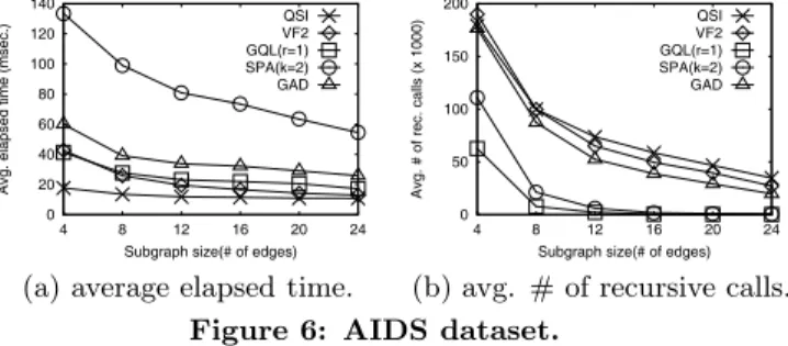
Figure 6: AIDS dataset.
The average number of recursive calls for every algorithm decreases as we increase the query size. Thus, all algorithms behave well despite their inherent exponential time complex-ity by choosing good join orders and by exploiting effective pruning rules. In terms of the average number of recursive calls, the ranking order is GraphQL, SPath, GADDI, VF2, and QuickSI. GraphQL and SPath exploit signature-based pruning before callingSubgraphSearch, and thus, the size
of the candidates (i.e., the search space) is the smallest. Note that the number of recursive calls for GraphQL is 6.7 and 6.4 smaller than those for QuickSI and VF2, respectively.
However, in terms of the average elapsed time, the rank-ing order is completely different. QuickSI is the fastest algo-rithm. VF2, GraphQL, GADDI and, SPath are 1.73, 1.99, 2.88, and 6.62 times slower than QuickSI on average, respec-tively. We analyze this surprising phenomenon in depth as follows: Although the average number of recursive calls for VF2 is 1.05 times smaller than QuickSI, the average cost of recursive calls for VF2 is 2.82 times larger than that of QuickSI. This is due to QuickSI’s optimized design of
IsJoinableas we pointed out in Section 3.4. In GraphQL,
the filtering time spent for GraphQL neighborhood signa-ture based filtering and pseudo-isomorphism based pruning constitutes 63.16% of the total elapsed time while the filter-ing time for QuickSI is zero. Note that the filterfilter-ing is exe-cuted before starting to callSubgraphSearch. In addition,
the average cost of recursive calls for GraphQL is 1.94 times larger than VF2. This is because 1) the query optimization time of GraphQL constitutes 10.6% of SubgraphSearch
since the sizes of query graphs are relatively large compared with the sizes of data graphs, and 2) GraphQL does not use any pruning rule forRefineCandidates.
In SPath, the filtering time spent for SPath neighbor-hood signature based filtering constitutes 61.23% of the to-tal elapsed time. The average cost of recursive calls for SPath is 5.18 times larger than that of GraphQL due to the overhead in path-based matching. Furthermore, the larger size of SPath neighborhood signature, compared to the GraphQL neighborhood signature leads to slower read-ing times for accessread-ing data graphs. In GADDI, for each query, calculating NDS distances for every pair of vertices of the query graph is very expensive. The average cost of recursive calls for GADDI is 3.76 times larger than that of GraphQL since the data graphs are sparse, and thus the NDS distances are often equal to zero, which does not help to refine candidates. Note that, unlike GraphQL and SPath, there is no additional filtering step for GADDI.
4.2 NASA Dataset
4.2.1 Database Construction
Table 3 shows the database size and database building times for all five algorithms using the NASA dataset. Note that the number of read I/Os for all algorithms is 3,077. The size of the database for QuickSI is 1.34 times large than that of VF2, since the sizes of the two B+-trees storing the frequency information become large due to the large number of unique labels (= 117,302). The size of the database for SPath is 5.85 times larger than VF2 since the value of neigh-borhood scopek0is set to four instead of two. Note that set-tingk0to four shows the best query performance for NASA. The increasing rate of GADDI over VF2 in NASA in terms of the database size and the elapsed time is smaller than that in AIDS since the average degree of NASA is smaller than that of AIDS. The GADDI was run with the shortest distanced= 1 and the neighborhood scopek0= 2.
Table 3: Database size and construction time for NASA dataset.
Alg. Size(MB) # of total I/Os Time(msec.)
VF2 44.04 8718 1697 QuickSI 58.99 10634 3769 GraphQL 57.65 10461 1950 SPath(k0=4) 257.68 36089 21737 GADDI 95.33 15288 32167
4.2.2 Query Processing
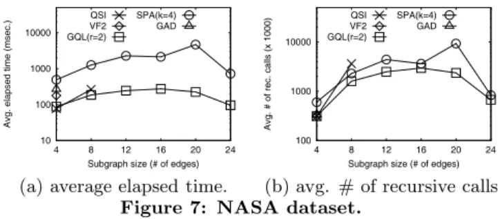
Figure 7 shows the subgraph isomorphism search perfor-mance using the NASA dataset. SPath was run with the best signature neighborhood scope k0 = 4, and GraphQL was run with the best refinement levelr= 2. The GADDI was run with the shortest distanced= 1 and the neighbor-hood scopek0= 2.
The purpose of this experiment is to see if those five algo-rithms exploit this important characteristics of the dataset. VF2,QuickSI, and GADDI show exponential behaviors at the sizes of query sets 8, 12, and 8, respectively. Only GraphQL and SPath complete their query execution in a reasonable time. This striking phenomenon is due to the se-rious problems both in their join order selection and in the absence of signature-based pruning. To verify our claim,
10 100 1000 10000
4 8 12 16 20 24
Avg. elapsed time (msec.)
Subgraph size (# of edges) QSI
VF2 GQL(r=2)
SPA(k=4) GAD
(a) average elapsed time.
100 1000 10000
4 8 12 16 20 24
Avg. # of rec. calls (x 1000)
Subgraph size (# of edges) QSI
VF2 GQL(r=2)
SPA(k=4) GAD
(b) avg. # of recursive calls.
Figure 7: NASA dataset.
we first changed the join orders of QuickSI with those of GraphQL for some slow queries, and this modified version of QuickSI completed these queries in a reasonable time. We note that QuickSI uses statistics for label frequencies for all data graphs in the database while GraphQL and SPath use statistics for label frequencies for each data graph. Thus, GraphQL and SPath can generate a better join order than QuickSI for these queries. However, for the other slow queries, especially, those having star-shaped subgraphs with many same labeled vertices, although QuickSI uses the join orders of GraphQL, it still shows exponential behavior. Note that QuickSI compares one query vertex with one data ver-tex at a time, and thus, it tries to explore all combinations of query vertices and data vertices of the same label for such star-shaped subgraphs. However, GraphQL and SPath can efficiently prune such subgraphs if query vertex signatures are not contained in the corresponding data vertex signa-tures. Thus, both GraphQL and SPath efficiently process such star-shaped queries, significantly reducing the number of candidates. This indicates that we need to combine good join order strategies with signature-based pruning for the NASA query/data sets.
It should be noted that, at the query sizes 20, unlike GraphQL, SPath shows jumps both in the number of recur-sive calls and the elapsed time. This is due to serious prob-lem in its join order selection. However, at the query size 24, we observe that signature-based pruning significantly prune candidate sets. For example, u∈V(q)|C(u)| for the 61st query of size 24 is 71.01 times smaller thanu∈V(q)|C(u)| for the 61st query of size 20. Thus, in spite of the inherent problem in join order selection of SPath, the elapsed time of SPath significantly is reduced for the query size 24 by exploiting the signature-based pruning of SPath.
The average number of recursive calls for GraphQL in-creases as we increase the query size up to 16. This is due to search space increments. However, when we increase the query size further, the average number of recursive calls de-creases. This phenomenon is explained as follows. As we increase the size of a query, the search space also increases. However, when a larger query has vertexes having infrequent labels, the signature-based pruning of GraphQL significantly prunes candidates, thereby significantly reduce the average number of recursive calls.
In terms of the average elapsed time, the performance of GraphQL is 10.38 times faster than SPath on average since 1) the loading time including in-memory signature construc-tion time for GraphQL is 5.55 times faster than that for SPath, 2) the filtering time for GraphQL is 2.45 times faster than that for SPath since SPath usesk0= 4, and 3) the to-tal cost of recursive calls for GraphQL is 14.33 times smaller than that for SPath. Note that settingrto two in GraphQL filters the number of candidates very effectively. In order to
compensate for the lack of the additional filtering step using pseudo-subgraph isomorphism of the GraphQL algorithm, we have to use a larger neighborhood scope (k0=4) for the SPath algorithm. Thus, u∈V(q)|C(u)| of SPath is 1.21 times smaller than that of GraphQL. However, due to the overhead of computing a larger SPath neighborhood signa-ture, the filtering time of SPath is 2.45 times larger than that of GraphQL.
4.3 Yeast Dataset
In this experiment, we use three types of query sets: sub-graph, clique, and path. The query sets of the first type are generated as is done for AIDS. The other types of query sets are provided by the original authors of GraphQL. The query sets of the second type contain clique queries (com-plete graphs) that correspond to protein complexes. The queries of the last type correspond to biological pathways. The vertices of the last two types are randomly assigned with the top 40 most frequent vertex labels, and each query graph vertex has only one label. Note that, unlike subgraph queries, path and clique queries do not satisfy the contain-ment relationship since they are randomly generated.
4.3.1 Database Construction
Table 4 shows the database sizes and database building times for all five algorithms using the Yeast dataset. The SPath database is built with the best neighborhood scope
k0 = 1. That is, a larger neighborhood scope (i.e.,k0 >1) decreases the query performance of SPath due to the over-head of larger SPath neighborhood signatures, which is con-trary to [18] suggesting a larger neighborhood scope for bet-ter query performance. The GADDI was run with the short-est distanced= 1 and the neighborhood scopek0= 2.
Note that the number of read I/Os for all algorithms is 33. The size of the database for QuickSI is 2.58 times large than that of VF2, because of the large size of the B+-tree storing the frequencies. In the Yeast dataset, each vertex has 7.55 labels on average. Therefore the number of all distinct triples (source vertex label, edge label, target ver-tex label) which we need to store in a B+-tree can increase quadratically3. The size of the database for SPath is 9.02 times larger than that of VF2 since the number of triples
(d, l, c) in the SPath neighborhood signature and the
num-ber of adjacency lists in the SPath adjacency list increase with the average number of vertex labels. The increasing rate of GADDI over VF2 in terms of the average elapsed time is much larger than that for the AIDS dataset since the number and the cost of NDS distance calculations in-crease due to the larger degree of Yeast. Note that the cost of calculating an NDS distance depends on the size of the neighborhood. The increasing rate of GraphQL over VF2 in Yeast in terms of the database size and elapsed time is larger than that of AIDS because of the larger average degree and multiple labels for each vertex.
4.3.2 Subgraph Queries
The purpose of this experiment is to analyze the trends in query performance for Yeast using the same query gener-ation technique as for AIDS and NASA datasets. We used ten subgraph query sets with sizes ranging from one to ten. These query sets have the same containment property as for AIDS and NASA.
3i.e., =O(the average number of vertex labels)2
Table 4: Database size and construction time for Yeast dataset.
Alg. Size(MB) # of total I/Os Time(msec.)
VF2 0.41 89 46
QuickSI 1.07 175 378
GraphQL 2.03 296 284
SPath(k0=1) 3.73 514 437
GADDI 0.91 152 25272
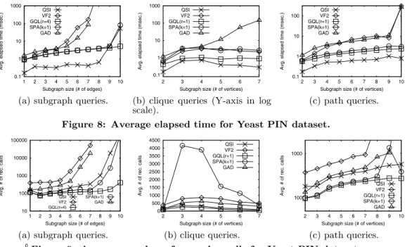
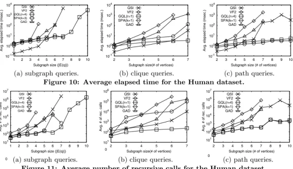
Figure 8(a) and Figure 9(a) show the subgraph isomor-phism search performance using subgraph queries for Yeast dataset. SPath was run withk0= 1, and GraphQL was run withr = 4. Note that if we increase k0 further, the query performance decreases due to the increased filtering cost. The GADDI was run withd= 1 andk0= 2. Only QuickSI, GraphQL, and SPath complete their query execution in a reasonable time. VF2 and GADDI show exponential behav-ior at query sizes nine and eight, respectively. This is due to the combined factors of increased search space and inefficient join ordering strategies of both algorithms. The average number of recursive calls increases with the size of queries. Note that such a trend is different from the results of the experiments on AIDS and NASA datasets. In terms of aver-age elapsed time, QuickSI is the fastest algorithm until query size eight. However, on average, QuickSI, SPath, GADDI, and VF2 are 2.20, 3.78, 5.89, and 369.50 times slower than GraphQL, respectively. Although QuickSI is designed for handling small graphs, it often outperforms the more re-cent algorithms GraphQL and SPath which are designed for handling large graphs. This indicates that signature-based pruning might not be very effective for the Yeast dataset. To analyze this phenomenon, we calculate the size of u∈V(q)|C(u)| for QuickSI, GraphQL, and SPath. The size ofu∈V(q)|C(u)|for QuickSI is only 2.01 and 2.78 times larger than those for SPath and GraphQL on average, re-spectively. However, increased filtering and loading times of SPath and GraphQL negate the advantage of signature-based pruning.
4.3.3 Clique Queries
Figure 8(b) and Figure 9(b) show the subgraph isomor-phism search performance using clique queries for the Yeast dataset. We use the same parameter values as used in sub-graph queries except for settingr= 1.
The average number of recursive calls for every algorithm increases as we increase the query size until three or four, then it decreases, if we increase the query size further. This trend is similar to that for NASA. Thus, all algorithms be-have well despite their inherent exponential time complex-ity by choosing good join orders and by exploiting effective pruning rules. In terms of the average number of recursive calls, the ranking order is GraphQL, QuickSI, GADDI, VF2, and SPath.
In terms of the average elapsed time, the ranking order is QuickSI, GraphQL, VF2, SPath, and GADDI. This is due to the lower cost of a recursive call of QuickSI and VF2. Note that, although the numbers of recursive calls of GraphQL and SPath decrease as we increase the size of queries from five to seven, the elapsed times of GraphQL and SPath slightly increase. This is due to increasing over-head of filtering in GraphQL and SPath. As for GADDI, since the data graphs are dense, the comparison costs based on the NDS distance and the shortest path exponentially
0.1 1 10 100 1000 1 2 3 4 5 6 7 8 9 10
Avg. elapsed time (msec.)
Subgraph size (# of edges) QSI
VF2 GQL(r=4) SPA(k=1) GAD
(a) subgraph queries.
0.1 1 10 100 1000 2 3 4 5 6 7
Avg. elapsed time (msec.)
Subgraph size (# of vertices) QSI
VF2 GQL(r=1) SPA(k=1) GAD
(b) clique queries (Y-axis in log scale). 0.1 1 10 100 2 3 4 5 6 7 8 9 10
Avg. elapsed time (msec.)
Subgraph size (# of vertices) QSI VF2 GQL(r=1) SPA(k=1) GAD (c) path queries.
Figure 8: Average elapsed time for Yeast PIN dataset.
10 100 1000 10000 100000 1 2 3 4 5 6 7 8 9 10
Avg. # of rec. calls
Subgraph size (# of edges)
0 QSI VF2 GQL(r=4) SPA(k=1) GAD
(a) subgraph queries.
0 500 1000 1500 2000 2500 3000 3500 4000 4500 2 3 4 5 6 7
Avg. # of rec. calls
Subgraph size (# of vertices) QSI VF2 GQL(r=1) SPA(k=1) GAD (b) clique queries. 100 1000 2 3 4 5 6 7 8 9 10
Avg. # of rec. calls
Subgraph size (# of vertices) QSI VF2 GQL(r=1) SPA(k=1) GAD (c) path queries.
Figure 9: Average number of recursive calls for Yeast PIN dataset.
crease as the size of a query increases. Thus, GADDI shows the worst performance in terms of the average elapsed time.
4.3.4 Path Queries
Figure 8(c) and Figure 9(c) display the subgraph isomor-phism search performance using path queries for the Yeast dataset. We use the same parameter values as used in sub-graph queries except for settingr= 1.
The performance results of all the algorithms increase as the query size increases. In terms of the average elapsed time, the ranking order is QuickSI, GraphQL, SPath, GADDI, and VF2. This is because 1) QuickSI generates reasonably good join orders for path queries, and 2) the cost of a recur-sive call for QuickSI is the lowest. In terms of the average elapsed time, QuickSI is 2.53, 3.22, 56.96, and 65.12 times faster than GraphQL, SPath, GADDI, and VF2 on average. The VF2 and GADDI algorithms show exponential behav-iors at query size ten because of the serious problems in their join order selection.
4.4 Human Dataset
4.4.1 Database Construction
Table 5 shows the database sizes and database building times for all five algorithms. Note that the number of read I/Os for all algorithms is 148. SPath was run withk0= 3 for subgraph queries. Otherwise, it was run withk0 = 1. The GADDI was run withd= 1 andk0= 2. The ratio of the size of a QuickSI database over a VF2 database is 1.11, which is smaller than the ratio for the Yeast dataset. This is due to the smaller number of distinct vertex labels. Since this dataset has a larger average degree than Yeast, the database sizes of GraphQL and SPath are 5.27 and 13.58 times larger than that of VF2. Due to a larger degree than Yeast, the cost of calculating NDS distances sharply increases, and thus, the ratio of the building time of GADDI over VF2 accordingly increases compared with that for Yeast.
4.4.2 Subgraph queries
Figures 10(a) and 11(a) show the results of subgraph iso-morphism search test using subgraph queries for the Human
dataset. SPath was run withk0= 3, and GraphQL was run withr= 4. The GADDI was run withd= 1 andk0= 2.
Table 5: Database size and construction time for Human dataset.
Alg. Size(MB) # of total I/Os Time(msec.)
VF2 1.55 349 93 QuickSI 1.72 373 964 GraphQL 8.13 1193 774 SPath(k0=1) 11.28 1596 1669 SPath(k0=3) 17.09 2340 3323 GADDI 4.88 775 624265
In terms of the average elapsed time and the average num-ber of recursive calls, the performance of all algorithms in-creases as the query size inin-creases. Although QuickSI shows the best performance in terms of the average elapsed time until the query size four, all algorithms except GraphQL fail to complete the subgraph queries due to their exponential behaviors at query sizes five, seven, eight, and eight for VF2, GADDI, QuickSI, and SPath, respectively. This is due to 1) the increasingly large search space size with increasing query sizes and 2) the join order selection problem. Note that this dataset has a higher density and fewer unique vertex labels than those of Yeast.
4.4.3 Clique and Path Queries
Figures 10(b) and 11(b) show the performance results for the clique queries. Figures 10(c) and 11(c) show the perfor-mance results for the path queries. We also use the same parameter values except for setting r = 1 and k = 1 for clique queries and settingr= 4 andk= 1 for path queries. The performance trend of both types of queries for the Human dataset is similar to that of path queries for the Yeast dataset. The only notable difference is that, in path queries, the performance of QuickSI at query size ten is bet-ter than that at query size nine. This is because QuickSI fortunately selects better join orders at query size ten.
5. CONCLUSION
In this paper, we provide a fair comparison of subgraph isomorphism algorithms by using a common framework. We