University of Nebraska - Lincoln
DigitalCommons@University of Nebraska - Lincoln
Sociology Department, Faculty Publications Sociology, Department of
2012
Macrostructure from Microstructure: Generating
Whole Systems from Ego Networks
Jeffrey A. Smith
University of Nebraska-Lincoln, [email protected]
Follow this and additional works at:http://digitalcommons.unl.edu/sociologyfacpub Part of theSocial Statistics Commons, and theSociology Commons
This Article is brought to you for free and open access by the Sociology, Department of at DigitalCommons@University of Nebraska - Lincoln. It has been accepted for inclusion in Sociology Department, Faculty Publications by an authorized administrator of DigitalCommons@University of Nebraska - Lincoln.
Smith, Jeffrey A., "Macrostructure from Microstructure: Generating Whole Systems from Ego Networks" (2012).Sociology Department, Faculty Publications. 247.
Generating Whole Systems from Ego Networks
Macrostructure from Microstructure: Generating Whole Systems from Ego Networks* Jeffrey A. Smith, Duke University
Word Count 15668
* Please send all correspondence to Jeffrey A. Smith at [email protected]. The key questions in this paper emerged out of discussion with Miller McPherson. James Moody, Lynn Smith-Lovin, Robin Gauthier and the network working group at Duke also provided helpful feedback. The author would also like to thank James Moody for providing the code and assistance to create the Sociology Coauthorship network used in this paper. Parts of this paper were presented at the 2011 Sunbelt Social Networks Conference. This research uses data from Add Health, a program project designed by J. Richard Udry, Peter S. Bearman, and Kathleen Mullan Harris, and funded by a grant P01-HD31921 from the Eunice Kennedy Shriver National Institute of Child Health and Human Development, with cooperative funding from 17 other agencies. Special
acknowledgment is due Ronald R. Rindfuss and Barbara Entwisle for assistance in the original design. Persons interested in obtaining data files from Add Health should contact Add Health, Carolina Population Center, 123 W. Franklin Street, Chapel Hill, NC 27516-2524
Bio: Jeffrey Smith is a doctoral candidate in sociology at Duke University. His research focuses on networks, quantitative methodology and stratification. He is particularly interested in
1 Macrostructure from Microstructure: Generating Whole Systems from Ego Networks
Abstract:
This paper presents a new simulation method to make global network inference from sampled data. The proposed simulation method takes sampled ego network data and uses Exponential Random Graph Models (ERGM) to reconstruct the features of the true, unknown network. After describing the method, the paper presents two validity checks of the approach: the first uses the 20 largest Add Health networks while the second uses the Sociology Coauthorship network in the 1990’s. For each test, I take random ego network samples from the known networks and use my method to make global network inference. I find that my method successfully reproduces the properties of the networks, such as distance and main component size. The results also suggest that simpler, baseline models provide considerably worse estimates for most network properties. I end the paper by discussing the bounds/limitations of ego network sampling. I also discuss possible extensions to the proposed approach.
2 1. INTRODUCTION
Global network measures are notoriously difficult to measure with sampled, or incomplete, information. It is difficult to describe the cohesion (Moody 2004), group structure (Frank and Yasumoto 1998) or diffusion potential (Watts 2002) of a network if we cannot capture the direct and indirect connections among all individuals.1
Unfortunately, it is often practically impossible to collect full network data on many populations of interest. For example, it may be impossible to interview everyone in a very large network, while an electronic (or easily collected) data source may not exist (Lewis et al. 2008). A smaller network may also prove difficult if one has limited resources or if the population is not institutionally bounded (e.g. adolescents in schools). The problem only becomes worse if one is interested in multiple networks at different locations. In short, while we may be interested in global network features, it is often impossible to collect complete data on the population of interest.
This paper offers a new, practical approach for researchers interested in global network structure where only sampled data can be collected (Frank 1971; Granovetter 1976). There are a number of ways to sample a network, including subgraph (Frank 1971) and snowball sampling (Goodman 1961; Handcock and Gile 2010; Koskinen, Robins and Pattison 2010), but this paper focuses on the simplest possible option—an independent sample of ego networks (Marsden 1987; Krivitsky, Handcock, and Morris 2011). Here, respondents are randomly sampled from the population and describe themselves and their local social network. Ego network data are easy to collect and
1 Complete census data are, however, unnecessary to make inference about most network statistics (Borgatti, Carley and Krackhardt 2006; Kossinets 2006).
3 already found on many social surveys. It is, unfortunately, often infeasible to analytically estimate network properties from ego network data, and past studies have typically used simulation instead (Lee 2004; Morris et al 2009).
This study builds on the ego network simulation tradition, offering a new method for global network inference. The approach takes ego network data and uses two models, Exponential Random Graph Models (Robins et al. 2007) and case control logistic
regression (McPherson, Smith and Smith-Lovin 2011), to generate full networks
consistent with the sampled data. The method also assumes that the size of the network is known. The simulated networks are then used to estimate the features of the true network. Intuitively, ego network data are drawn randomly from the population: any network consistent with the sampled information is thus a possible construction of the true network.
The method extends past work by exploiting the sampled information more fully. The simulation is built around a new measure of ego network structure, as well as more traditional measures, like homophily. The measure of ego network structure captures the full distribution of ego network types, and is thus more precise than existing options. The paper also assess the validity of the proposed method on known networks.
I begin the paper with background sections on network sampling, simulation and ego network data. I then describe my method of generating full networks from ego network data. I follow the methods section with two validity checks. The first check uses data from the National Longitudinal Study of Adolescent Health, or Add Health, a nationally representative study of adolescents covering grades 7-12 in 1994-1995 (Harris
4 2009). The analysis uses the 20 largest Add Health networks (N between 1000 and 2200) and compares the estimates produced by my method with the empirically known values. I test my method on a series of network features, including typical measures of
connectivity (e.g. distance) and clustering (e.g. modularity). The paper then moves to a larger network, describing the same analysis on the Sociology Coauthorship network in
the late 1990’s (~60,000 nodes).
2. A SHORT SUMMARY OF NETWORK SAMPLING
Much of the work on network sampling stems from the pioneering analysis of Frank (Frank 1971; 1977; 1978a). Frank derived formulas to estimate network-level measures from a sample (Frank 1971; 1978b). The formulas were often based on a random sample of nodes in the network, or a subgraph sample, where all ties between sampled respondents are recorded. Unfortunately, a subgraph sample is impractical for many, if not most, network settings. For example, a subgraph sample on a large network may yield few, or even zero, ties between sampled respondents unless the sample is very large or the density is very high. A subgraph sample without ties tells the researcher the network is not very dense, but not much else.
As an alternative, researchers have employed sampling schemes that capture more local information, such as ego network sampling (Marsden 1987) and snowball sampling (see Thompson and Frank 2000; Handcock and Gile 2010; Koskinen et al. 2010;
Goodman 2011). Both of these sampling strategies record local tie information, thus avoiding the large N problem of subgraph samples. In a snowball sample, researchers
5 interview respondents, the friends of respondents, the friends of the friends, and so on.2 Snowball sampling avoids the limitations of subgraph sampling but is quite complex in its own right—as one must identify, find, and interview the associates of the respondents. Additionally, a snowball sample is not easily embedded in an existing survey.
Ego network data, in contrast, are easy to collect and already widely used by network scholars (e.g. Moore 1990; McPherson, Smith-Lovin and Brashears 2006). The survey randomly samples individuals from a known population (i.e. the population is not hard-to-reach). The survey then gathers information about the respondents and their local social network: we know the number of associates, or alters, per respondent; the
characteristics of those alters; the characteristics of the respondent; and the presence of ties between alters.3 The ego networks are completely independent and the alters are not identified. Ego network data are also easily added to existing surveys, even if that survey was not designed with networks in mind. The promise of ego network sampling is thus considerable: for it becomes possible to make global network inference from data that are, potentially, already at hand (or at least easily collected).
I design my method with these practical issues in mind, focusing solely on an ego network sampling scheme (Marsden 1987). I do, however, consider snowball sampling more thoroughly in the conclusion, noting where the extra information from a snowball sample will be particularly useful.
2 We can assume here that the population is not hard-to-reach (e.g. not sex workers) (Heckathorn 2011). The initial respondents can then be randomly sampled from a known sampling frame (Goodman 2011), although the initial respondents can also be drawn from a convenience sample (see Goodman 2011and Handcock and Gile 2011 for a more detailed discussion).
6 Past work on ego network sampling has employed simulation techniques as a means of analysis, and the proposed method follows in this simulation tradition (Morris and Kretzschmar 2000; Lee 2004; Lee 2008; Morris et al. 2009). Simulation based inference is an ideal option as analytical solutions are infeasible: one can explore the properties of the network by generating full networks consistent with the local ego network information. It is important to recognize that the generated networks are consistent with the local information in the sample, but need not, necessarily, be consistent with the macro properties of the true network. Despite this limitation,
simulation methods can produce excellent approximations of the full network: for ego network data provide a surprisingly large amount of information about the network.
Some network types will yield more accurate estimates than others, however, and I describe the networks most appropriate for the simulation method in the conclusion.4 Briefly, the method will be most appropriate for networks that exhibit homophily (as the simulations rely on group mixing patterns), are undirected (as there is no asymmetry information) and capture strong tie relationships (as it is impractical for a respondent to list every person they know or recognize).
3. EGO NETWORK DATA AND THE SIMULATION APPROACH
The proposed method proceeds in three steps. First, it calculates the local information available from the sampled data. Second, it uses the local information to simulate full networks consistent with the sampled data. And third, it uses the generated
4 It is important to note that many of these limitations are practical limitations, and not theoretical ones. The limitations may be less restrictive under different sampling schemes and I discuss possible extensions in the conclusion.
7 networks to calculate the statistics of interest. The key to the simulation approach is extracting the maximum amount of information from the sample.
Ego network data provide information on the local social world of respondents, but also provide a wealth of information about the full, unknown network from which the ego networks were drawn. At the simplest, an ego network sample provides
compositional information about the true network. Respondents answer basic
demographic questions, thus providing a count of males/females, blacks/whites, etc. in the network.5
More importantly, ego network surveys ask respondents to nominate their alters.6 The list of alters provides an estimate of the degree distribution, or the number of alters per person.7 The list of alters also provides information on differential degree, or the average degree by demographic group (as we know the demographic characteristics of the respondents). Some surveys may employ a truncated naming scheme, where a respondent can name a maximum of X alters (say 10). A truncated naming scheme will yield biased estimates of the degree distribution (although one could possibly simulate, or project, the truncated part). I assume, for the sake of this paper, that that the degree distribution is not truncated: respondents are allowed to name a small but non-trivial number of alters.8
5 The alter demographic information is not used in the calculation. I do not use the alter information as the alters do not represent a random sample of the population.
6 Respondents describe their alters but do not formally identify them.
7 The alter-alter ties are not used when calculating the degree distribution. I do not include the alter ties as they do not capture the true degree of the alters—who could have ties to individuals not included in the respondent’s ego network.
8
I have, however, performed supplementary robustness checks on a set of Add Health networks (not reported here for space considerations). I compared the estimates produced under truncation to those
8 Ego network data also provide information about homophily. Respondents report on their own demographic characteristics as well as the characteristics of their alters. The paired respondent/alter information captures the demographic similarity among social contacts.9
The measures described so far, including composition, degree distribution, differential degree and homophily, can be measured unbiasedly from ego network data. The measures are unbiased as they depend on node or dyad level information, and thus do not depend on information outside the ego network. Past sampling/simulation studies have measured homophily and the degree distribution from ego network data and used those estimates to generate full networks consistent with the sampled data (Lee 2008; Morris et al. 2009; Krivitsky, et al. 2011).
Past simulation methods have made less use of the structural information, which captures the pattern of social ties among alters. In ego network data, the respondent describes the relationship between each alter pair (is there a tie between alter one and two, one and three…?). This structural information has rarely been the focus of past
produced under no truncation. I first took random ego network samples from the largest five Add Health networks. With the truncation sample, I only allowed respondents to name up to 10 friends (rather than full amount, where the maximum is upwards of 25). The sampled data yielded a biased degree distribution, and I thus tried to “fill out” the truncated part before running the simulation. Specifically, I took those with 10 alters and assigned them a value equal to or above 10. I assigned the value by taking draws from a negative binomial distribution (with shape and mean parameters that yielded a distribution closest to the empirical distribution, after the full simulated distribution was truncated to 10 or lower). After I assigned those with 10 alters a value equal to or above 10, I ran the simulation method, generating estimates for the macro network features of interest. I then compared those estimates to the estimates produced with the full degree distribution. The results are, on the whole, quite similar between the two sets, although the truncated results yield slightly higher bias for distance based measures and for the triad census.
In interpreting these results, one must bear in mind that my analysis ignores the measurement error induced by the original study design—where individuals were only allowed to nominate a limited number of male and female friends. It is possible that the bias in my analysis would have been larger if the “true” network
(with no truncating in the original design) had been available.
9 The alter-alter ties are not considered in the homophily measurement as the alters do not comprise a random sample of the population.
9 work, although some studies have discussed the limitations of the data (Newman 2003; Grannis 2010). For example, transitivity (where a friend of friend tends to be a friend) is estimated inaccurately because it depends on information outside the ego network, such as the degree of the named alters (Soffer and Vazquez 2005; Bansal, Khandelwal and Meyers 2009). In a similar manner, we cannot estimate the rate of assortative degree mixing, or the tendency for individuals with similar degree to be socially tied.
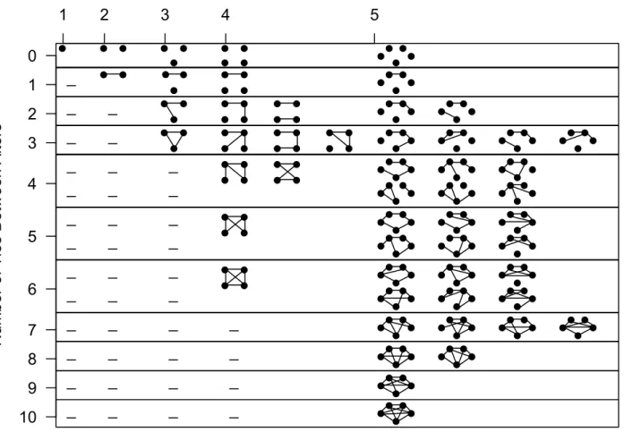
Given these limitations, this paper offers a new measure of ego network structure that makes the most of the available data.10 Specifically, I take the alter-alter tie data and form a distribution of ego network patterns, or a distribution of ego network
configurations (see Holland and Leinhardt 1976 and Middendorf et al. 2005 for related intuition).11 Figure 1 summarizes the 53 possible ego network configurations of size 5 and below (see Freeman 1979). The distribution of ego network configurations is formed by placing each respondent in the appropriate structural category. Ego networks are placed in a unique category based on three attributes: size; the degree distribution among alters (ignoring ego); and the number of triangles (ignoring ego).12 We can write this formally as:
10The simplest structural measure is local density, or the number of ties in the ego network relative to the
number possible (ignoring ego in the calculation). Local density can be averaged over all cases (with degree greater than two) to calculate the clustering coefficient, or the mean local density (Watts and Strogatz 1998). The clustering coefficient, unfortunately, proves a poor measure for my purpose. There may be many sets of ego networks that have the same overall mean density but different structural patterns across the ego networks. Average density thus does not offer a precise enough measure, or signal, of ego network structure, so that we cannot easily compare the structural types in the generated networks to the sampled data.
11 Note that the alter-alter ties are used to construct the ego network configurations but are not used in the homophily or degree distribution measures (see note 7 and 9).
12 These three pieces of information will uniquely identify the configuration for small ego networks (i.e. less than six). For larger ego networks, the three measures will reduce the number of possible
10 𝐿𝑒𝑡 𝑋 𝑏𝑒 𝑎 𝑠𝑞𝑢𝑎𝑟𝑒 𝑚𝑎𝑡𝑟𝑖𝑥 𝑜𝑓 𝑑𝑖𝑚𝑒𝑛𝑠𝑖𝑜𝑛𝑠 𝑚 𝑥 𝑚, 𝑐𝑜𝑛𝑠𝑖𝑠𝑡𝑖𝑛𝑔 𝑜𝑓 𝑡ℎ𝑒 𝑎𝑙𝑡𝑒𝑟𝑠 𝑖𝑛 𝑡ℎ𝑒 𝑒𝑔𝑜 𝑛𝑒𝑡𝑤𝑜𝑟𝑘 𝑜𝑓 𝑟𝑒𝑠𝑝𝑜𝑛𝑑𝑒𝑛𝑡 𝑝. 𝐿𝑒𝑡 𝑋 = 1 𝑖𝑓 𝑎 𝑡𝑖𝑒 𝑒𝑥𝑖𝑠𝑡𝑠 𝑏𝑒𝑡𝑤𝑒𝑒𝑛 𝑎𝑙𝑡𝑒𝑟 𝑖 𝑎𝑛𝑑 𝑎𝑙𝑡𝑒𝑟 𝑗. 𝐷𝑒𝑓𝑖𝑛𝑒 𝑒𝑔𝑜 𝑛𝑒𝑡𝑤𝑜𝑟𝑘 𝑐𝑜𝑛𝑓𝑖𝑔𝑢𝑟𝑎𝑡𝑖𝑜𝑛 𝑝 𝑏𝑦 𝑡ℎ𝑒 𝑢𝑛𝑖𝑞𝑢𝑒 𝑐𝑜𝑚𝑏𝑖𝑛𝑎𝑡𝑖𝑜𝑛 𝑜𝑓: ⎩ ⎪ ⎨ ⎪ ⎧1. 𝑆𝑖𝑧𝑒𝑝= 𝑚 2. (𝑑𝑖)𝑝= 𝑋𝑖+, 𝑤ℎ𝑒𝑟𝑒 𝑑𝑖 𝑖𝑠 𝑡ℎ𝑒 𝑑𝑒𝑔𝑟𝑒𝑒 𝑜𝑓 𝑎𝑙𝑡𝑒𝑟 𝑖 (1) 3. 𝑇𝑝 = 𝑋𝑖𝑗∗ 𝑋𝑗𝑘∗ 𝑋𝑖𝑘 , 𝑤ℎ𝑒𝑟𝑒 𝑡 𝑖𝑠 𝑡ℎ𝑒 𝑠𝑒𝑡 𝑜𝑓 𝑎𝑙𝑙 𝑡𝑟𝑖𝑎𝑑𝑠 𝑖𝑛 𝑋. 𝑡 = 𝑡123, 𝑡124, … , 𝑡(𝑖−2),(𝑖−1),𝑖 . 𝑡
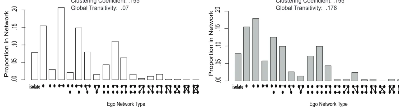
Figure 2 offers two example distributions. The figure plots the proportion of (hypothetical) respondents in each ego network category.13 The left hand panel plots the ego network distribution from a random network (with a specified degree distribution), while the right hand panel plots the ego network distribution from a clustered network—
where there are group divisions and moderate transitivity. It is clear from this simple example that networks with different structural features yield very different ego network distributions (see Johnsen 1985 for this same idea applied to the triad distribution).
(Figure 1 about here)
More generally, the ego network distribution is a reflection of the larger network: for the distribution faithfully mirrors the data generating process and captures the
structural heterogeneity across respondents. For example, the distribution captures the structural heterogeneity around size, where smaller ego networks may be denser than larger ego networks. The distribution also captures more subtle heterogeneity, where ego
increases non-linearly as size increases). For simplicity, I focus on smaller configurations, although a researcher may, in practice, have alter tie information for a large number of alters (i.e. more than five). Also note that it is possible to know the total number of alters but collect alter-alter tie data for a subset of all alters.
11 networks of the same size and density may have very different structural patterns.14 The
measure’s precision is ultimately crucial for the simulation: for the algorithm uses the distribution to choose between seemingly similar networks. A simple density score would obscure such differences.
(Figure 2 about here)
More substantively, the ego network distribution serves as a latent signal for many properties not captured by ego network data. For the same underlying forces that structure the real network (e.g. structural balance) similarly constrain the ego network configurations. Simulated networks with the right ego network patterns are thus shaped by the same local processes as the real network, and are thus more likely to have the right structural features—even if those features are not directly captured by the individual level data.
For example, a network with the right ego network configurations is likely to have the right level of transitivity, even though ego network data cannot directly measure transitivity without bias. The key is fitting the entire ego network distribution, where the local clustering patterns (by degree) aggregate to create global transitivity. We can see this in Figure 3, which plots the ego network distributions from two networks with the same local density (i.e. the density of the ego networks) but different levels of global transitivity. The ego network distributions are significantly different across the two networks. The ego network distribution thus differentiates the networks in terms of
12 transitivity, even though the ego networks offer the same direct, local estimate of
clustering.
(Figure 3 about here) 4. METHODS: BACKGROUND
The methods section is divided into two parts. In the first section, I describe the models employed during the simulation, Exponential Random Graph Models (ERGM) and case control logistic regression. In the second part, I describe the simulation process itself.
4.1. ERGM
ERGMs are statistical models used to test hypotheses about the structural features of a network (Holland and Leinhardt 1981; Frank and Strauss 1986; Wasserman and Pattison 1996; Snijders et al. 2006; Handcock et al. 2008). Formally, for each pair of
actors, or nodes, i,j in the set N (N=1,2…n), let Yij= 1 if there exists a tie from i to j and Yij=0 if no tie exists (all Yii are definitionally assumed to be zero). Yij=Yji in undirected networks (the focus in this paper). Furthermore, let yij be the observed values of Yij while
y is the observed, or realized, network. Y is then a random graph on N, where each possible network tie may be seen as a random variable Yij. The ERG models the Pr(Y=y) to capture the structural features of the network. The independent variables are counts of network measures (e.g. number of edges) and take a variety of forms, including
individual, dyadic and higher order terms (Robins et al. 2007; Goodreau, Kitts and Morris 2009). We can write the model as:
𝑃(𝒀 = 𝒚) =𝑒𝑥𝑝 𝜃 𝑔(𝒚)
13 where 𝑔(𝒚) is a vector of network statistics, 𝜃 is vector of parameters, and 𝜅(𝜃) is a normalizing constant.
ERG models are particularly useful for testing hypotheses about the formation, or generation, of a network, but can also be used to simulate networks (Robins, Pattison, and Woolcock 2005). The model coefficients measure the strength of various micro processes shaping the formation of the network. One can take those coefficients and (stochastically) predict the presence or absence of a tie between pairs of people.
Traditionally, ERG models have been estimated on full networks without missing data, but more recent work has extended the model to sampled data. For example,
Handcock and Gile (2010), estimated ERG models under a two wave link tracing design (or a snowball sample on a not hard-to-reach population—Goodman 2011). They
compared the estimated parameters from the sample to the parameters from the complete network (N=36), finding the bias to be relatively small. In a similar manner, Koskinen et al. (2010) introduced a Bayesian approach for estimating ERGMs with missing data. Unlike Handcock and Gile (2010), they also used the ERGM coefficients to make
inference about global network measures: where the estimated parameters were first used for missing link prediction;; once the missing data was “filled in”, the network was used to calculate various measures of interest, such as betweenness. They also considered their model in the context of snowball sampling on a not hard-to-reach population.
Both papers estimated the properties of a network from sampled data, and thus had similar goals as this paper. The sampling schemes employed by Handcock and Gile (2010) and Koskinen et al. (2010) are, however, more complex than the ego network
14 sampling scheme considered here. Still, the work on snowball sampling highlights a crucial idea: if one can estimate parameters from sampled data, the model can be used to simulate networks based on the estimated coefficients.
Past work on ERG models and ego network sampling has explored this idea (primarily) using degree and homophily terms (Morris et al. 2009; Krivitsky et al. 2011). For example, Morris et al. (2009) used an ERGM to simulate sexual networks from ego network data, including terms in the model for racial mixing, differential degree and the degree distribution. Sexual ego network data do not provide configurational information (i.e. did the alters share other sexual partners?) and the model was specified without a local clustering term (transitivity, for example). The parameters could then be estimated from ego network data and used to simulate synthetic networks. A degree/homophily approach is appropriate for sexual networks as the structure is likely to be captured through the degree distribution, differential degree and mixing rates.15 A model without a local clustering term is not, however, appropriate for many other network types of interest—say a friendship network, where there is strong transitive closure.
4.2. Case Control Logistic Regression
The case control framework is used for two tasks: to estimate homophily on the ego network data; and, more crucially, toupdate the homophily coefficients as the
15
Heterosexual networks are unlikely to have strong tendencies towards local clustering. It is unlikely, for example, for two women to share multiple male partners (so we see chains rather than diamonds). Thus a researcher could afford to not explicitly model local clustering and still capture the global structure of the network—as most of the clustering in the network would be induced, or captured, by correctly modeling group mixing at a macro level.
15 simulation progresses. This ensures that the simulated networks reflect the empirical level of homophily.
Past work on network sampling has typically used log-linear models to estimate homophily (Mare 1991; Morris 1991). Log-linear models compare the frequency of observed ties between categories (e.g. blacks and whites) to the frequency expected by chance. Log-linear models are limited, however, as it is difficult to include a large number of predictors (especially if they are not categorical). Given this practical limitation, McPherson et al. (2011) introduced an extended log-linear model based on case control models. Case control methods are employed in medical research to study rare events, such as having cancer, which are difficult to capture with random sampling (Breslow and Day 1980). Instead, case control methods take the cases, those individuals with the disease, and compare them to individuals without the disease, or the controls, on some behavior or condition of interest (such as smoking).
The case control method is a natural fit for ego network data. Rather than take a random sample of dyads, ego network data capture the rare event of interest, the social ties between individuals. We can then view the cases, or those dyads with a social
relationship, as the respondent-alter ties in the ego network data. The controls, in turn, are dyads that do not have a social relationship. The controls are formed independent of the cases and need not come from the same data source. It is, however, typical to create the controls by randomly pairing respondents together, thus capturing random mixing in the population, or chance expectations. In this case, the “0s”, or non-ties, are a random sample of respondent-respondent dyads.
16 The case control model compares a behavior, or condition, between the cases and the controls. Here the condition of interest is the social distance between i and j in each dyad: for example, absolute distance on age or match/no match on race. For categorical variables, social distance can also take the form of a mixing matrix. A mixing matrix describes the frequency of ties between all categories, where there is one term for every combination of categories a pair could fall into (e.g. black-white, white-white…). The social distance between respondents and alters is then compared to the social distance between individuals in the control part of the dataset. The model takes the form of a
logistic regression, where the “1s” are the respondent-alter pairs and the “0’s” are those
pairs where a tie does not exist. Formally we can write the model as:
ln 1 − 𝑝𝑝(𝑶()𝑶) = 𝜃𝑜𝐗 (3) where 𝑂 is the presence or absence of a tie; 𝑋 is the social distance between i and j for each dyad, and 𝜃𝑜 is the vector of coefficients. The case control model is conceptually close to a dyadic independent ERGM, where both models compare the counts of dyadic properties (e.g. matching on race) to the level expected by chance (see Koehly, Goodreau and Morris 2004 for a related discussion). There are, however, important estimation differences between the models. In an ERGM, chance expectations are constructed from all individuals in the network. In the case control models, chance expectations are constructed independently from the network tie information. Thus, an ERGM on the ego networks would include the alter information in the random baseline, while the case control model would not.
17 More generally, the case control model offers a great deal of flexibility: because the controls are separate from the cases, the controls can easily be constructed to
represent a different comparison. The case control model is ultimately useful because of this flexibility, making it easier to update the homophily coefficients as the simulation proceeds.
5. METHODS: THE SIMULATION APPROACH 5.1. Setup and Assumptions
The proposed simulation approach uses ERGM and case control logistic
regression to generate full networks from ego network data.16 I divide the discussion of the method into three parts: gathering information prior to the simulation; setting up the simulation; and the simulation itself. In the first part, the method extracts the local information from the sampled data; in the second and third parts, the method generates networks consistent with the local information. And more specifically, the method searches for the “best” fitting network, using the empirical ego network distribution as the benchmark (while also maintaining the correct level of homophily). I present the method as a series of steps and offer a summary in Table 1.
For the purposes of discussion, assume that the ego network survey has
demographic information on the respondents and alters. Also assume that the researcher knows the number of alters per respondent, but can only ask alter-alter tie information for
16
I assume that all ERGM estimation and simulation is done in R (2009) using the statnet package (Handcock et al. 2008). The formulas are specified with the statnet package in mind, although the model form is quite general. The case control models are also run in R.
18 a subset of the alters (e.g. for four randomly selected alters).17 Also assume that the size of the true network is known.
5.2. Gathering Information Prior to the Simulation
Step 1: Calculate the degree distribution and differential degree from the sampled data.
Step 2: Calculate the ego network configuration distribution from the sampled data (using Formula 1). See Figure 2 for an example.
5.3. Setting up the Simulation
Step 3: Simulate an initial network of size N (assumed to be known) with the same degree distribution as the sampled data (estimated in Step 1); also assign demographic characteristics to the nodes in the network.18 Specifically, nodes in the simulation are randomly assigned the demographic profile (e.g. black, college graduate) of someone in the sample with the same degree as themselves.19 The initial network will thus have the right size, degree distribution (estimated from the sampled data), and
17
The respondent burden increases non-linearly with the number of alters, and it is more realistic to cap the number of alter-alter tie questions. For example, an ego network of size five yields 10 questions while an ego network of size 10 yields 45 questions.
18 The initial simulation of the random network can be done within the ERGM framework, or alternatively, by using a stub based algorithm (Newman, Strogatz and Watts 2001; Viger and Latapy 2005)
19Technically, the demographic profiles are drawn from the set of individuals with +/-1 of the degree of
the focal node. I include a +/-1 bound for situations where the simulated network is much larger than the sample. Here, it may be the case that in the sample there are very few people with a given degree (say 12) but in the simulated network, with a much larger N, there may be many people with that degree. If one matched exactly by degree, everyone with degree 12 would look demographically the same. I add and subtract one to the degree value in order to induce some uncertainty into the demographic profile of these rare degree cases. This widens the pool, however slightly, of who can be selected for a given degree. One could alternatively draw from among respondents with the exact degree, x. The choice is not likely to be consequential.
19 demographic composition. The network will also reflect differential degree, where some demographic groups have higher degree than others.20
Step 4: Specify an ERG formula from which to simulate the full networks. The ERG formula determines which micro features are used to generate the full network. The model terms should thus capture all of the information available from ego network data: differential degree, homophily and the ego network configuration distribution. The initial coefficients for the terms are set in Step 5, while the degree distribution is handled separately as a constraint in Step 6.
Differential degree: include a nodecovariate term for initial degree, or the degree
of each node from the initial network (from Step 3). A nodecovariate term serves as a main effect: in this case, a tie is more likely if person i has high initial degree and less likely if person i has low initial degree (assuming a positive coefficient). The
nodecovariate term thus maintains the degree of node i throughout the simulations (with some stochastic variation). By holding expected degree constant, the nodecovariate term maintains the empirical correlation between degree and the demographic characteristics (as the demographic characteristics are held fixed and the empirical correlation is reflected in the initial network—see Step 3). Nodes falling into a given category in the simulation will thus have the same mean degree as that category in the sampled data.21
20 By assigning a node, i, with degree x, all of the demographic characteristics of a randomly selected person with that degree, the correlation between the demographic characteristics is maintained. Differential degree is also captured as demographic categories with high degree in the sample will be placed on high degree nodes in the simulated network. The network will also reflect the demographic composition of the population as individuals are randomly selected from the sample (from the set of people with the
appropriate degree).
21 Alternatively, it is also possible to use a series of nodefactor terms for each demographic characteristic observed in the data.
20
Homophily: One should also include homophily terms for each demographic
dimension available in the sampled data. An absolute difference term is appropriate for continuous variables, such as age, while a mixing matrix is appropriate for categorical
variables (“absdiff” or “nodemix” in the statnet package—Handcock et al. 2008). The mixing matrix for race, for example, may include terms for the number of black-black, black-white, white-white, etc. ties in the network.22 Formally, the count of black-white ties (for example) can be written as:
𝑌𝑖𝑗
𝑗∈𝑊 𝑖∈𝐵
2 , 𝑤ℎ𝑒𝑟𝑒 𝒀 𝑖𝑠 𝑎𝑛 𝑢𝑛𝑑𝑖𝑟𝑒𝑐𝑡𝑒𝑑 𝑛𝑒𝑡𝑤𝑜𝑟𝑘. (4)
Ego Network Configuration Distribution: The ego network configuration
distribution offers a more difficult specification problem than homophily or differential degree. There are a large number of configurations, and the model must include a term, or terms, that will reproduce the distribution in the simulated networks. One could include a term for each possible configuration, but this yields a very large number of (similar) clustering terms. Such a model is difficult to estimate and simulate from.
As an alternative, one could specify a model with a single clustering term. This specification has two key advantages: first, the model is considerably simpler; and second, the model is less likely to yield degenerate networks (Handcock 2003), likely under the dummy variable specification (i.e. one term for each configuration).23 The
22 The full mixing matrix is, under most circumstances, the ideal choice as it captures the pattern of ties across all categories. One could alternatively include a match-no match term for each category, effectively including the diagonal of the full mixing matrix. One could also include a simple match/no match term. 23 The simulations are degenerate when they put disproportionate weight on a few networks, often the full or empty graph (Handcock 2003).
21 question is what single term will yield non-degenerate networks with the right ego
network configuration distribution. There are a number of possible options, but I suggest that GWESP (geometrically weighed edgewise shared partner) is the most appropriate choice, where GWESP is a weighted summation of the shared partner distribution (Snidjers et al. 2006). Formally:
𝐺𝑊𝐸𝑆𝑃 = 𝑒 1 − (1 − 𝑒 ) 𝑝 (5) where 𝛼 is a scalar, determining the rate of decay on the summation (where lower values weight the initial shared partners to a much larger extent than the 10th, 11th, etc. shared partner) and 𝑝 is the number of dyads (with an edge) who have i partners in common. A GWESP coefficient is positive when pairs of tied nodes have a high number of shared partners (relative to chance). Substantively, GWESP captures transitivity and higher order clustering in the network (Hunter 2007).
GWESP is a particularly appropriate choice as it mirrors the structural features of the ego networks. For example, the shared partner distribution in an ego network (from
ego’s point of view) is equivalent to the degree distribution of the alters.24 The degree distribution of the alters is largely sufficient to differentiate the ego network
configurations, given size. Similarly, GWESP captures structural heterogeneity through the parameter, while the ego network configurations vary systematically by size. By decreasing , one implicitly decreases the density in larger ego networks relative to smaller ego networks (as adding another shared partner has a smaller effect and larger ego networks have a higher number of possible shared partners).
22 I suggest that GWESP is the most theoretically and technically appropriate option, but there is nothing inherent in the simulation that says GWESP must be used. A
researcher could easily specify another clustering term: for example, one term for each ego network configuration or a triangle term. I only suggest that GWESP is an ideal option; it is certainly not the only one.
Step 5: Set the initial coefficients for the terms specified in Step 4. The
nodecovariate coefficient, for example, must be positive, so that initial degree is highly correlated with final degree. A coefficient that is too large, however, limits the flexibility of the simulation.25 The initial homophily coefficients, defined as 𝜃𝑜, are set using case control logistic regression. The model predicts a tie as a function of social distance (as specified in Step 4).26
Unlike homophily or differential degree, the coefficient for the clustering term (e.g. GWESP) cannot easily be assigned: for it is not possible to analytically solve for the correct coefficient (i.e. the coefficient that will yield networks with the right ego network configuration distribution). The method thus generates an initial (naïve) value by
estimating a dyadic independent ERGM on the ego networks. The model predicts ties as
25 If the constraint on degree is too strong it becomes difficult to simultaneously satisfy other constraints. A value of .5 is appropriate, for example, although the exact value is not especially crucial.
26 One could alternatively estimate the initial homophily coefficients using a dyadic independent ERGM. The proposed method uses case control logistic regression as it is easier to exclude the alters from the baseline comparison, or the null, although the differences across models should be small (Koehly et al. 2004). The alters of the respondents do not represent a random sample from the population, and should thus be excluded when forming the baseline, which represents random mixing in the population.
23 a function of the specified term (e.g. GWESP), and the estimated parameter is used as the initial coefficient.27
Step 6: Set the constraints for the model. The model is constrained on the degree distribution, where only networks consistent with the observed degree distribution (from Step 1) have a non-zero probability of remaining in the set of generated networks.28
(Table 1 about here)
5.4. Simulation Procedure
Step 7: Simulate a network using the model specified in Steps 4-6. The simulation takes the network from Step 3 as the starting point.
Given the simulated network from Step 7, Steps 8-11 adjust the model to find a better fitting network, specifically updating the homophily coefficients and the
coefficient for the clustering term.
Step 8: Compare homophily in the simulated network (from Step 7) to homophily in the sampled data; update homophily coefficients if any error is found. The generated networks may have incorrect mixing rates due to the initial estimation process. The initial homophily model (see Step 5) only includes homophily terms, so that all non-homophily terms are implicitly set to 0. The simulation model, in contrast, is conditioned on a non-zero clustering term. The homophily estimates are therefore biased when they are used to
27 All of the respondents and all of their alters make up the network for the ERG model; although, of course, there will only be ties between respondents and alters.
24 simulate the network (as the initial estimates are not conditioned on the positive value for clustering) (Goodreau et al. 2009).29
The simulation method consequently checks for inconsistencies between the simulated network and the sampled data. The method then updates the homophily coefficients to adjust for any error. A coefficient is decreased if mixing is too strong in the simulated network (between category i and category j) and increased if mixing is too weak.
Formally, the homophily coefficients are updated using case control logistic regression. The method first takes the tied dyads from the simulated network and the respondent-alter dyads from the sampled data and creates a combined dataset. The dataset includes the demographic characteristics of person i and j in each dyad. A 0/1 indicator variable is then created, where the sample dyads are “1s” and the dyads from the
simulated network are “0s”. The method then runs a simple logistic regression, predicting 1s as a function of the social distance between i and j. The regression thus compares the social distance in the sampled data (between respondents and alters) to the social distance in the simulated network (among pairs where a tie exists). The estimated coefficients are then added to the original homophily coefficients, thus scaling the original homophily coefficients up or down, depending on the error in the simulated network. This procedure can be written formally as:
𝐶𝑜𝑛𝑠𝑡𝑟𝑢𝑐𝑡 𝑚𝑎𝑡𝑟𝑖𝑐𝑒𝑠 𝐴 𝑎𝑛𝑑 𝐷 𝑓𝑟𝑜𝑚:
1. 𝑎𝑙𝑙 𝑖, 𝑗 𝑅𝑒𝑠𝑝𝑜𝑛𝑑𝑒𝑛𝑡 𝐴𝑙𝑡𝑒𝑟 𝑝𝑎𝑖𝑟𝑠, 𝑑𝑒𝑓𝑖𝑛𝑒𝑑 𝑎𝑠 𝑅
29 The original homophily coefficients are not conditioned on GWESP or degree (or any term) for practical reasons. The initial homophily estimates are updated throughout the simulation procedure, and this is facilitated by having unbiased initial estimates, which is far easier to calculate when GWESP is set to 0.
25 2. 𝑎𝑙𝑙 𝑖, 𝑗 𝑝𝑎𝑖𝑟𝑠 ∈ 𝑆 == 1 𝑤ℎ𝑒𝑟𝑒 𝑆 𝑖𝑠 𝑡ℎ𝑒 𝑠𝑖𝑚𝑢𝑙𝑎𝑡𝑒𝑑 𝑛𝑒𝑡𝑤𝑜𝑟𝑘. 𝐴 = 0, 𝑖𝑓 𝑖, 𝑗 ∉ 𝑅1, 𝑖𝑓 𝑖, 𝑗 ∈ 𝑅𝑖𝑗 𝑖𝑗 𝐷𝑛 = 𝑆𝑜𝑐𝑖𝑎𝑙 𝐷𝑖𝑠𝑡𝑎𝑛𝑐𝑒 𝑏𝑒𝑡𝑤𝑒𝑒𝑛 𝑖 𝑎𝑛𝑑 𝑗 ln 1 − 𝑝𝑝(𝑨()𝑨) = 𝜃𝑎𝐃 (6) 𝜃 = 𝜃 + 𝜃
where 𝜃 is the original homophily coefficients, 𝜃 is the vector of estimated
coefficients, and 𝜃 is the updated homophily coefficients. For categorical variables (e.g. a racial mixing matrix), 𝜃 will be positive when the simulated network has too few ties for that term (e.g. black-white ties) and will be negative when the simulated network has too many. And more generally, 𝜃 measures the upward or downward error in the original homophily coefficients: for 𝜃 compares the empirical level of homophily to the homophily generated by 𝜃 , conditioned on the other terms in the model. By adding 𝜃 to
𝜃 , the coefficients are brought back into line with the proper values.
Step 9: Simulate a new network using the updated coefficients from Step 8 (starting from the network in Step 7 and using the model formula from Step 4 and 6). Steps 8 and 9 are repeated a small number of times to ensure that homophily is correct in the simulated network.
Step 10: Evaluate the ego network configuration distribution in the simulated network (from Step 9). The generated network from Step 9 will have the correct degree distribution and mixing patterns, but need not, necessarily, have the right ego network configuration distribution. The simulation procedure thus allows the coefficient on the clustering term (e.g. GWESP) to vary, looking for networks that better fit the empirical
26 ego network distribution. The ego network configuration distribution is evaluated in this step, while the coefficient is updated in the next.
There are two steps to evaluating the ego network configuration distribution: first, calculating the ego network configuration distribution from the simulated network; and second, comparing the distribution from the simulated network to the distribution from the sampled data (calculated in Step 3). The method compares the distributions using Pearson’s chi square value:
(𝑂𝑖− 𝐸𝑖)2
𝐸𝑖 𝑛
𝑖=1
(7)
where 𝑂𝑖 is the observed frequency in the simulated network, 𝐸𝑖 is the empirical frequency, and n is the total number of possible configurations (53 in the five alter case). Larger chi square values indicate a worse fit, so that the ego networks in the simulated network do not structurally match the ego networks in the sampled data.
Step 11: Update the coefficient on the clustering term to find a better fitting network (given the chi square value from Step 10). A “better” network has a lower chi
square value, or has an ego network configuration distribution closer to the empirical distribution (estimated from the sampled data). The ego network configuration
distribution thus serves as the benchmark, or ruler, by which the generated networks are judged. The question is what coefficient on the clustering term will yield simulated networks with the lowest chi square value. In updating the model, the nodecovariate
27 coefficient is held constant, while the homophily coefficients are updated using the
framework from Step 8.30
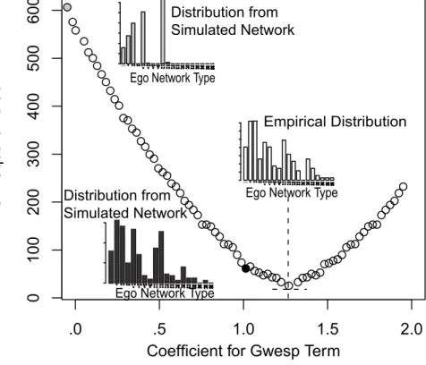
Figure 4 offers a snapshot of the minimization process. Assume, for this example, that the researcher has included a GWESP term in the model. The x-axis represents a (restricted) range of GWESP coefficients. The y-axis represents the chi-square value associated with that GWESP coefficient. The GWESP coefficient is used to simulate a network (along with the other terms in the model) and the chi square value is calculated from the simulated network. The optimization process moves away from points with high chi square values, like the “grey” distribution in Figure 4, and towards points, or
coefficients, with lower chi square values—like the “black” distribution in Figure 4. The
“black” distribution matches the sampled ego networks more closely and thus offers a better fit.
(Figure 4 about here)
I present two options for minimizing the chi square value. The first is a simple hill climbing algorithm. The algorithm moves the current coefficient in the positive and negative direction, looking for a better fitting network. For each potential move, the method takes the coefficients (from Step 9 but with the new coefficient for the clustering term) and simulates a network; the method also adjusts for homophily bias if necessary (Steps 7-9). The method then calculates the chi square value for each network, comparing the ego network distribution in the simulated networks to the distribution in the sampled data. The algorithm settles on whichever move maximizes the drop in chi square from the
30 One would introduce bias if the homophily coefficients are held constant as the coefficient on the clustering term is updated.
28 current coefficient. The method then returns to Step 7 and starts the process over again, using the new coefficients to simulate the networks. The search process ends when all local moves yield a worse chi square value than the current coefficients.
The second minimization process is similar to the hill climbing algorithm, but requires a less exhaustive search of the solution space. Under this option, the method first simulates a sample of networks at different values of the (clustering) coefficient—
specifically values above and below the starting coefficient. For each simulated network, the method adjusts for homophily bias and calculates the chi square value (i.e. Steps 7-10). The method then takes the coefficients for the clustering term and the chi square values and fits an OLS regression to the data. The regression predicts chi square as a function of a linear and quadratic term:
𝜒𝑖2 = 𝛽
0+ 𝛽1(𝐶𝑖)+ 𝛽2(𝐶𝑖)2 (8) where 𝜒𝑖2 equals the chi-square value for network i, and 𝐶
𝑖 equals the coefficient on the clustering term for network i. The regression coefficients are then used in an optimization routine. The method uses the Nelder-Mead algorithm to find the clustering term
coefficient with the lowest chi square value (based on the fitted regression line). The solution, or coefficient, is then used as the starting point for the next iteration. The method then repeats Steps 7-10 again, ending the process when the expected chi square value does not improve over the last iteration.
29 At the end of the search process, the method generates networks from the best set of coefficients.31 One then calculates the statistics of interest (e.g. component size) on the simulated networks and summarizes over the estimated values. The simulated networks yield a distribution of statistics, capturing the stochastic uncertainty in the estimates. Sampling error provides another source of uncertainty, and a researcher would have to perform a bootstrap analysis to take this into account.32
The simulation, in short, rests on a kind of approximated likelihood ratio test: the coefficients are updated to find a more likely full network, where a network is more likely if its ego network configuration distribution is closer to the empirical distribution (estimated from the sampled data). The simulation approach thus draws (implicitly) on formal statistical properties, increasing the probability that the generated networks
approximate the true network—as the method finds the most likely full network given the local data and the specified model. One could even run the simulations with different specifications of the clustering term, checking to see if the fit (i.e. chi square) improves under different models.
More generally, I argue that simulation based inference holds great promise: for social networks are highly constrained by size, the degree distribution, and
social/physical distance (Butts 2001; Faust 2006), all properties captured by the simulation. If the simulated networks correctly capture these constraining dimensions,
31It is possible that more than one solution will yield a “low” chi square value, so that the optimization curve plateaus as the chi square approaches its minimum. I take this uncertainty into account by simulating networks from a series of coefficients; specifically, I use coefficients with a chi square value within 30 of the lowest estimated chi square value.
32 One could take random samples from the original sample and redo the analysis. Each sample would yield multiple networks, and thus statistics, to summarize over. In the end, one would produce a final distribution by pulling the parameter estimates from each sample into one distribution.
30 then the space of possible networks is greatly reduced. The number of possible networks is reduced further by finding networks with the right ego network configurations. For the empirical ego networks are shaped by the same processes that shape the true network; a network consisting of the sampled ego networks thus represents a possible construction of the real network.
6. TESTING THE METHOD ON EMPIRICAL NETWORKS
6.1. Summary of the Analytical Strategy, Measures and Baseline Comparisons
I now present a set of empirical tests checking the validity of the method. For each test, I first sampled ego networks from a completely known, empirical network. I then applied my method to the sampled data and compared the properties of the generated networks to the properties of the real network. I examined the accuracy and variability of the estimates and compared my results with those of simpler, baseline models. I tested my method on the 20 largest Add Health networks and the Sociology Coauthorship network in the 1990’s. The Add Health networks ranged from 1000 to 2200 students and varied in structure and composition, offering a robustness check for the method (see McFarland et al. 2009). The Coauthorship network offered a different type of test: here the method was used on a relatively large, highly transitive network (N~60000).
The network properties of interest were divided into two broad categories: connectivity and clustering/group structure. For connectivity, the measures included size of the largest component and bicomponent, where a component is a set of nodes
connected by at least one path (a path exists if two nodes are reachable through a series of adjacent ties). Bicomponent size is the largest set of people connected by at least two
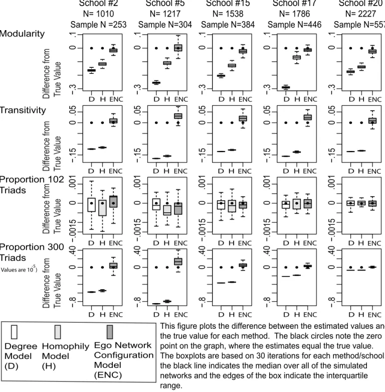
31 independent paths (Moody and White 2003). There were also measures for reachability and mean distance, where distance is the length of the shortest path between any two nodes (restricted to reachable pairs). Reachability was measured as the proportion of people reachable 5 steps out into the network (averaged over all starting nodes). The analysis used modularity as the measure of group structure. I used the group detection algorithm of Clauset, Newman and Moore (2004) to divide the network into groups. I then calculated modularity on the found groups, where modularity measures the strength of group divisions in the network; modularity is high when there are many ties within groups and few between (Newman 2006).33 The analysis used transitivity and the triad census as the measures of clustering. Transitivity is the relative number of two-step paths that also share a direct link. The triad census was measured as the proportion of 102 triads, or triads with one symmetric tie, and the proportion of closed triads, or 300 triads (Cartwright and Harary 1956).34
The proposed method estimates the global features of a network from sampled ego network data; it is possible, however, that simpler, existing methods will produce equally valid results. I thus compared my method to two baseline models. The first model generated random networks with the correct size and degree distribution (Newman et al.
33I do not contend that the Clauset et al. (2004) algorithm is the best, or most appropriate, group detection
method available. I simply need a consistent way of finding groups and the Clauset et al. (2004) algorithm is fast and serves my purpose. Formally, modularity equals:2𝑚1 ∑𝑖𝑗 𝑌𝑖𝑗−𝑘2𝑚𝑖𝑘𝑗 𝛿 𝑐𝑖, 𝑐𝑗 ,
𝑤ℎ𝑒𝑟𝑒 𝑘 𝑖𝑠 𝑡ℎ𝑒 𝑑𝑒𝑔𝑟𝑒𝑒 𝑜𝑓 𝑛𝑜𝑑𝑒 𝑖, 𝑚 𝑖𝑠 𝑡ℎ𝑒 𝑛𝑢𝑚𝑏𝑒𝑟 𝑜𝑓 𝑒𝑑𝑔𝑒𝑠 𝑖𝑛 𝑡ℎ𝑒 𝑛𝑒𝑡𝑤𝑜𝑟𝑘, 𝑌, 𝑐 𝑖𝑠 𝑡ℎ𝑒 𝑔𝑟𝑜𝑢𝑝 𝑡ℎ𝑎𝑡 𝑛𝑜𝑑𝑒 𝑖 𝑖𝑠 𝑎𝑠𝑠𝑖𝑔𝑛𝑒𝑑 𝑡𝑜 𝑎𝑛𝑑 𝛿 𝑖𝑠 𝑡ℎ𝑒 𝐾𝑟𝑜𝑛𝑒𝑐𝑘𝑒𝑟 𝑑𝑒𝑙𝑡𝑎 𝑠𝑦𝑚𝑏𝑜𝑙.
34 The triad distribution represents a somewhat different comparison than the other measures: for the triad distribution is directly captured by the test statistic in the algorithm, the ego network configuration distribution. The other measures, e.g. bicomponet size, are less directly tied to the test statistic, as the sampled data provide no explicit information about these non-local measures. Thus a “good” model will reproduce the triad census but not necessarily the other network measures.
32 2001).35 This model is called the Degree (D) model in the figures and tables. The second baseline model incorporated homophily into the Degree model, capturing both the degree distribution and the pattern of group mixing. This model is called the Homophily model in the tables and figures (H). The full model included the degree distribution, homophily and the newly introduced ego network configuration distribution. I refer to my own method as the Ego Network Configuration Model (ENC).
The three models are directly nested. This makes it possible to discuss the “value added” for each term in the model. The question is whether the ego network
configuration distribution is necessary to produce good estimates, or if homophily and the degree distribution are sufficient.
6.2. Add Health Networks: Data, Sampling and Models
Add Health is a nationally representative survey of public and private schools covering grades 7-12. Students were asked to nominate up to five male and five female friends. The constructed, symmetrized networks were used in two sets of analyses. The networks were symmetrized using a “weak” rule: if there was a directed link between i and j or a directed link between j and i, then i and j were tied in the undirected network.
The first analysis used the 20 largest networks and randomly sampled 25 percent of the students within each school. The 25 percent sample results were used to compare across models. In the second analysis, I focused solely on my method, exploring the bias and sampling variability of the estimates under different sample sizes. I limited the analysis to
35 The networks can be generated within an ERGM framework (Handcock and Morris 2007) or from a stub-based algorithm (Viger and Latapy 2005). I use a stub based algorithm for the sake of convenience. The stub based algorithm takes the degree distribution as input and does not require any estimation prior to the simulation.
33 the five largest networks but considered sampling rates of 10 percent, 25 percent, 50 percent and 75 percent. I varied the sample size to test my method under more or less favorable samples.
Each sampled student provided the following information: first, the number of alters and the ties between alters; second, the characteristics of the respondent; and third, the characteristics of the alters. The characteristics included grade, race, sex, and club affiliations. Club affiliations were limited to broad categories: music, sports and academic. The survey was “realistic” as I only recorded alter characteristics and alter-alter ties for up to five friends, although there was no limit on the number of friends one could name. The five friends were randomly selected from the set of all friends for that respondent.36 The respondent described the ties between the randomly selected friends and answered questions about their demographic characteristics. The decision to use five friends was made independent of the Add Health study design. I used five alters for two reasons: first, it makes counting the ego networks more tractable; and second, it is more realistic for data collection purposes, where respondent burden is kept to a reasonable amount.
The simulation method requires an ERG model and I included the following terms in the formula: nodemix terms for grade, race, gender and club affiliation; a
nodecovariate term on initial degree; and GWESP.37 The simulations were also
36 I made no distinction between male or female friends and simply drew five people from the whole set of friends.
34 constrained on the degree distribution. The Homophily model was equivalent but did not include GWESP.
My method takes the model formula and initial coefficients and produces estimates for the statistics of interest. The analysis captured the variability of the
estimates by repeating the procedure 30 times for each school, starting with a new sample of ego networks for each iteration.38 There were parallel analyses for the baseline models (under 25 percent sampling).
6.3. Sociology Coauthorship Network: Data, Sampling and Models
The second validity check used the Sociology Coauthorship network as the empirical, known network. I constructed the network from article level data drawn from Sociological Abstracts. The database includes information on all sociology related articles going back to 1963, but the network was restricted to articles published between 1995 and 1999. An edge existed in the network if person i and person j coauthored a paper between 1995-1999. The empirical network included 60098 people and I worked with a random sample of 5 percent of the network. I produced estimates for only one sample due to the computational burden of the analysis (where a network of that size and transitivity requires a rather extended run time). I thus did not consider sampling
variability for the Coauthorship network.
As with Add Health, the hypothetical survey collected the following information: the number of alters (with no limit); the ties between alters (for five randomly selected alters); the characteristics of the respondent; and the characteristics of the alters (for five
38 A larger sample would be preferable but not reasonable given the number of networks and the run time of my algorithm—at minimum 1-2 hours for a network of size 1500.
35 randomly selected alters). The characteristics included gender, prestige (defined as
having ever published in AJS, ASR, or Social Forces), subfield specialty, and
quantitative/qualitative identification. I specified an ERG model with mixing terms for each characteristic as well as a nodecovariate term for initial degree. The model also included a GWESP term.39 All simulations were conditioned on the degree distribution. The Homophily model was exactly the same but did not include the GWESP term. 7. RESULTS
7.1. Qualitative Comparison
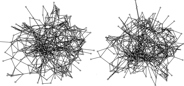
The results section begins with a qualitative comparison, showing that the
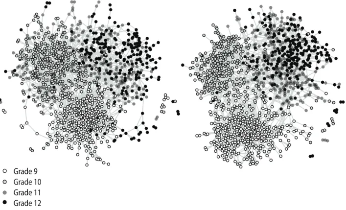
simulation produces realistic looking networks. Figure 5 offers a snapshot comparison for one typical Add Health network. The left hand panel presents the true network while the right hand panel presents one realization from the simulation process.40 The networks, while not identical, are strikingly similar—the macro structure in the real network is reflected in the overall shape of the simulated network. The comparison is similarly encouraging in Figure 6, which presents a more detailed view of the network. Here the figure is limited to nodes in grade 9. The simulation performs well even at this more fine grained level, generally reproducing the core-periphery structure of the grade 9 network.
Given these positive qualitative results, I now move to a more formal test of the approach. I first compare my results to those of simpler models. I then examine my model in more detail, looking at the results at different levels of sampling. In both
39 The parameter is allowed to vary during the simulation.
40 The network figures were produced in R using the sna package (Butts 2010). The nodes were originally placed using the Fruchterman-Reingold force-directed algorithm. The networks were then rotated to maximize comparability between figures—so that grade level was roughly located in the same position in each figure for Figure 5.
36 sections, the results begin with the connectivity measures before moving to clustering and group structure.
(Figure 5 and Figure 6 about here)
7.2. Connectivity: Baseline Model Comparisons
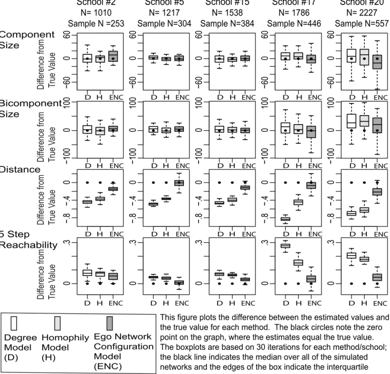
The connectivity results begin with the Add Health networks (under 25 percent sampling). It is difficult to visually summarize the results over all 20 networks. I simplify the presentation by focusing on five typical networks of different sizes. Figure 7 presents the results for my model as well as the baseline models. For each model (and measure), the analysis subtracts the empirical value from the estimated values from the 30 samples. The figure presents these differences in a series of box plots. The black dot marks the zero point, where there is zero difference between the true and estimated value. The paper offers more precise information about bias and sampling variability in Appendix A (where bias is the difference between the mean estimate and the true value). For each measure and network, the tables report the bias and the proportion bias (bias divided by the true value). The tables also report the standard deviation of the sampling distribution. See Tables A1-A8 for the 25 percent sample results.
It is clear from Figure 7 that all three methods successfully estimate the size of the largest component and bicomponent. For example, my method yields an average bias less than 1 percent of the true bicomponent size (across all networks). The simpler models also perform well. The Homophily and Degree models are thus good options if one is only interested in component or bicomponent size.