Nonparametric Methods
Aonan Zhang
Submitted in partial fulfillment of the requirements for the degree
of Doctor of Philosophy
in the Graduate School of Arts and Sciences
COLUMBIA UNIVERSITY
Aonan Zhang All Rights Reserved
Composing Deep Learning and Bayesian
Nonparametric Methods
Aonan Zhang
Recent progress in Bayesian methods largely focus on non-conjugate models featured with extensive use of black-box functions: continuous functions implemented with neural networks. Usingdeep neural networks, Bayesian models can reasonably fit big data while at the same time capturing model uncertainty. This thesis targets at a more challenging problem: how do we model general random objects, including discrete ones, using random functions? Our conclusion is:many (discrete) random objects are in nature a composition of Poisson processes and random functions. Thus, all discreteness is handled through the Poisson process while random functions captures the rest complexities of the object. Thus the title: composing deep learning and Bayesian nonparametric methods.
This conclusion is not a conjecture. In spacial cases such as latent feature models , we can prove this claim by working on infinite dimensional spaces, and that is how Bayesian nonparametric kicks in. Moreover, we will assume some regularity assumptions on random objects such as exchangeability. Then the representations will show up magically using representation theorems. We will see this two times throughout this thesis.
One may ask: when a random object is too simple, such as a non-negative random vector in the case of latent feature models, how can we exploit exchangeability? The answer is to aggregate infinite random objects and map them altogether onto an infinite dimensional space. And then assume exchangeability on the infinite dimensional space. We demonstrate two examples of latent feature models by (1) concatenating them as an infinite sequence (Section2,3) and (2) stacking them as a 2d array (Section4).
Besides, we will see that Bayesian nonparametric methods are useful to model discrete patterns in time series data. We will showcase two examples: (1) using variance Gamma processes to model change points (Section5), and (2) using Chinese restaurant processes to model speech with switching
List of Figures v
Part I Overview 1
Chapter 1 Introduction 2
1.1 A classical theory for random partitions . . . 2
1.2 Existing theory on latent feature models . . . 4
1.2.1 LFMs as random partitions . . . 5
1.2.2 LFMs with randomly permuted features . . . 6
1.3 Correlated LFMs . . . 8
Part II Composing Deep Learning and Bayesian Nonparametric Methods in Latent Feature Models 9 Chapter 2 Markov Mixed Membership Models 10 2.1 Model Description . . . 12
2.1.1 Markov mixed membership models . . . 12
2.1.2 Relationship to tree-structured models . . . 13
2.1.3 Related work . . . 14
2.2 Scalable Variational Inference . . . 15
2.2.1 Local variables . . . 16
2.2.2 Global variables. . . 17
2.2.3 Stochastic variational inference . . . 18
2.3 Experiments . . . 19
2.3.1 Document modeling . . . 19
3.1 Feature Allocation via Sequences . . . 26
3.2 Markov Latent Feature Models . . . 28
3.2.1 A parametric model . . . 28
3.2.2 A nonparametric model . . . 29
3.2.3 Application to a linear Gaussian model . . . 30
3.2.4 Discussion . . . 30
3.3 Inference . . . 30
3.3.1 Batch Variational Inference . . . 31
3.3.2 Stochastic Variational Inference . . . 34
3.4 Experiments . . . 36
3.4.1 HGDP-CEPH Cell Line Panel . . . 36
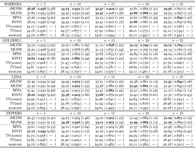
3.4.2 Image denoising . . . 38
Chapter 4 Random Function Priors for Correlation Modeling 40 4.1 Zas a random matrix? . . . 43
4.2 Zas a random measure. . . 44
4.2.1 Population random measure embedding . . . 44
4.2.2 Construction via completely random measures. . . 45
4.3 An illustration on topic modeling . . . 45
4.3.1 The model . . . 45
4.3.2 Amortized variational inference . . . 47
4.3.3 Network architectures . . . 49
4.4 Experiments . . . 50
4.4.1 Batch experiments . . . 50
4.4.2 Online experiments. . . 52
4.5 Discussion . . . 54
4.5.1 Connections with other random objects . . . 54
4.5.2 Deep hierarchical Bayesian models . . . 54
4.5.3 Posterior inference bottleneck . . . 55
Modeling 61
Chapter 5 Deep Bayesian Nonparametric Tracking 62
5.1 Motivations . . . 63
5.2 The Model . . . 64
5.2.1 Basic setup: Dynamic matrix factorization . . . 64
5.2.2 Variance gamma process onW . . . 65
5.2.3 Temporal tracking inH and data generation . . . 66
5.2.4 Extension: A deep likelihood model . . . 66
5.3 Variational inference . . . 67
5.3.1 Linear Gaussian observational model . . . 67
5.3.2 Extension: Variational auto-encoder model . . . 68
5.4 Further discussion . . . 70
5.4.1 Modeling velocity and acceleration of drift . . . 71
5.4.2 Prediction . . . 71
5.5 Experiments . . . 72
5.5.1 Methods and evaluations . . . 72
5.5.2 Stock market crash and recovery, 2008-2012 . . . 73
5.5.3 NFL tweets . . . 76
5.6 Conclusion . . . 77
Chapter 6 Fully Supervised Speaker Diarization 79 6.1 Motivations . . . 79
6.2 Baseline system using clustering . . . 81
6.3 Unbounded interleaved-state RNN . . . 82
6.3.1 Overview of approach . . . 82
6.3.2 Details on model components. . . 83
6.3.3 MLE Estimation. . . 85
6.3.4 MAP Decoding . . . 86
6.4 Experiments . . . 87
6.4.1 Speaker recognition model . . . 87
6.4.2 UIS-RNN setup . . . 87
6.4.5 Results . . . 88
6.5 Conclusions . . . 90
Part IV Inference for Bayesian Nonparametric Models 91 Chapter 7 Stochastic Variational Inference for the HDP-HMM 92 7.1 Motivations . . . 92
7.2 The HDP-HMM . . . 94
7.2.1 Stick-breaking construction . . . 94
7.3 Variational inference for the HDP-HMM . . . 96
7.3.1 The state transition matrix . . . 97
7.3.2 A local lower bound usingq(sd|zd) . . . 97
7.3.3 Mapping atoms between DP levels . . . 99
7.3.4 Stochastic variational inference . . . 99
7.4 Experiments . . . 100
7.4.1 Artificial data . . . 100
7.4.2 Alice’s Adventures in Wonderland . . . 102
7.4.3 Million Song dataset . . . 104
7.5 Conclusion . . . 106
7.6 Appendix . . . 106
Bibliography 109
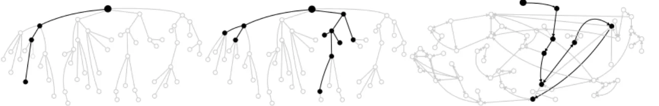
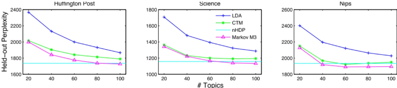
Figure 2.1 Comparison between three path-based models. (Left) The tree-structured nested Chinese restaurant process (nCRP) selects one path per group; (Mid.) the tree-based nested hierarchical Dirichlet process (nHDP) places high probability on a subtree for each group; (Right) the proposed graph-based Markov mixed membership model selects one path per group using a Markov random walk on the fully connected set of nodes (an example high-probability connectivity is depicted in the background here). . . 12 Figure 2.2 Held-out perplexity results. The Markov transition model (Markov M3) overall
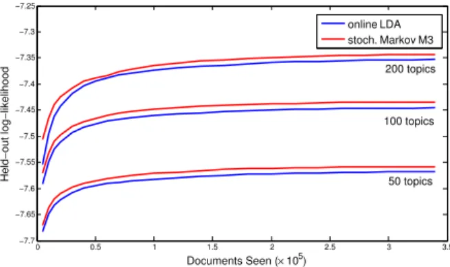
achieves best performance among parametric models. Its best performance is even better than the state-of-the-art nonparametric nHDP.. . . 19 Figure 2.3 Predictive performance for online Markov M3 and online LDA. Markov M3 is
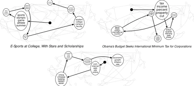
consistantly better for various number of topics through the entire learning process. . 20 Figure 2.4 Topic paths selected by three documents. The size of the node indicates the
proportion of the topic. . . 21 Figure 2.5 Selected topic subgraph from a 200-topic graph learned by online Markov M3
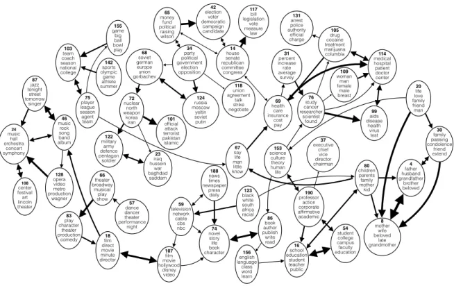
on New York Times dataset. The graph shows Markov transitions with high probability among topics. . . 22 Figure 2.6 Sensitivity analysis for (left) the truncation level of sticks, and (right) the
stick-breaking concentration parameter. Results are shown in terms of average log likelihood on a test set. . . 22
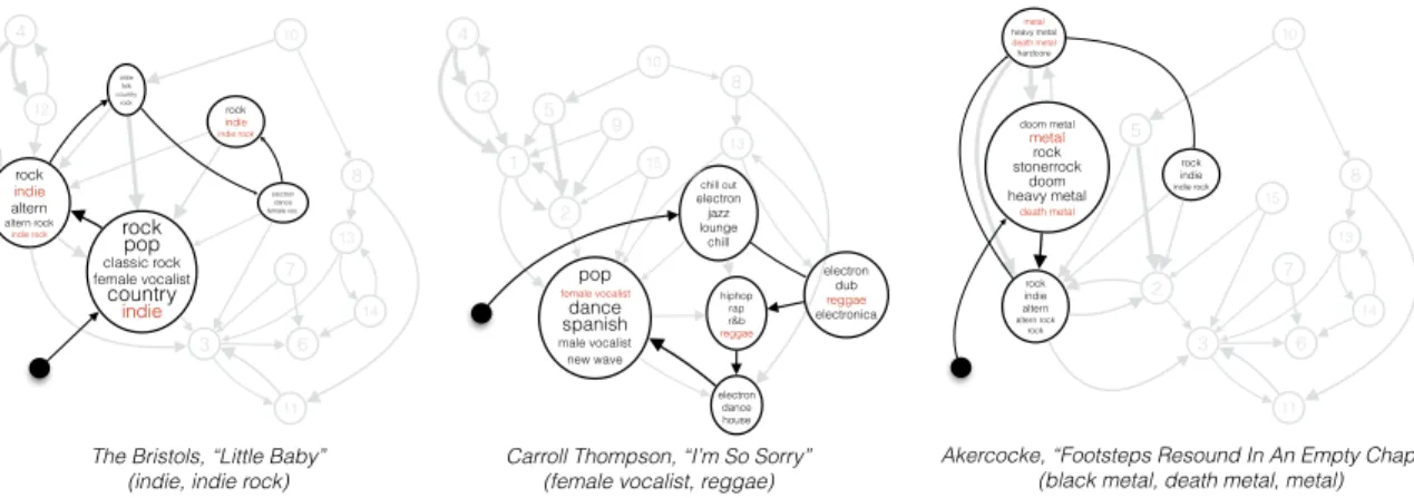
the initial state. The size of nodes indicates the proportion for that factor, and the thickness of arrows indicates the transition probability between factors. All the paths are embedded in the graph (the gray background). . . 23 Figure 3.1 An illustration of the construction of a 0-1 matrix from a sequential process,
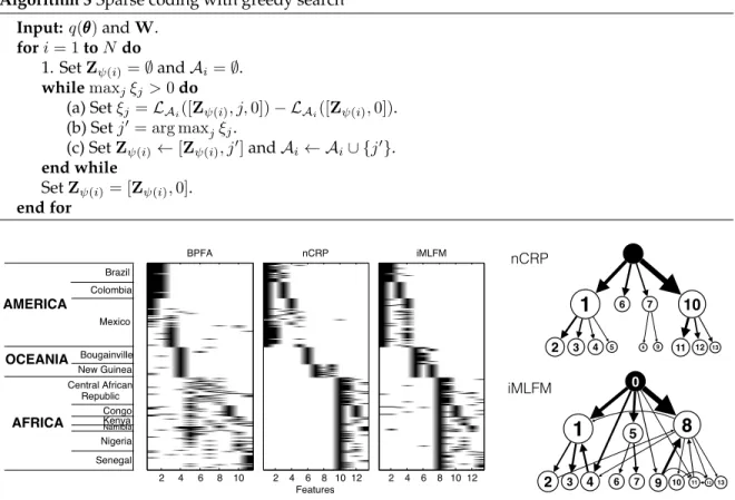
which we define to be a mixture of recurrent Markov chains. On the LHS, the chainZ starts from a null stateZ0= 0and generates four blocks (subsequences)Zψ(1)toZψ(4) by returning to 0 four times (shown as four colored paths on the graph). One the RHS, this sequence constructs a 0-1 matrix with four rows and the columns indicating the unique set of states visited in each block.. . . 27 Figure 3.2 (Left) Factors learned from BPFA, nCRP, and iMLFM on the HGDP-CEPH dataset.
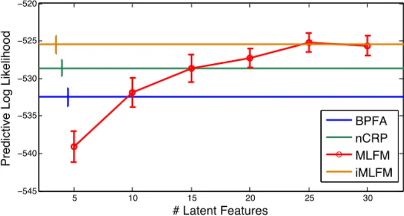
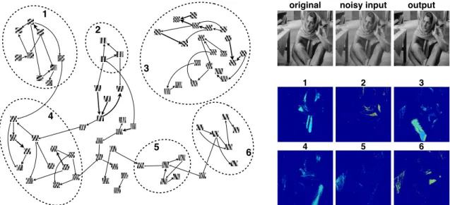
Observations from various regions are aligned vertically, as displayed on the left side. (Right) Graph learned from iMLFM and nCRP. . . 32 Figure 3.3 Average predictive result on HGDP-CEPH dataset. . . 36 Figure 3.4 (Left) A similarity-preserving 2-d embedded graph of the learned dictionary
elements using their transition probabilities. We show edges about a threshold, and the direction of an edge between two dictionary elements according to the higher transition probability. (Right) Feedback maps for dictionary elements in various regions in the graph on the left. . . 37 Figure 3.5 The four images used in our experiments. . . 38 Figure 4.1 Example of two equivalent representations: (left) Paintbox model for[Zn1, Zn2, Zn3]
by partitioning a unit square into eight regions, one for each distinct value. (right) Fac-torize the paintbox into three feature paintboxes, one each for a latent feature. Three examples ofunthat determineZnare demonstrated as dots in the partition paintbox, and as lines across feature paintboxes. . . 42 Figure 4.2 Decoupling a separately exchangeable discrete random measureξinto two parts. 43
generative process and dashed arrows show the VAE part of the posterior. We organize local parameters that belong to a document/word into boxes and remove all sub-indices. We use stochastic natural gradient ascent forθand use stochastic gradient ascent for
[`, V, g, f]. . . . . 47
Figure 4.4 (b) Left: The architecture we used in our experiments. Right: Various layer designs. 47 Figure 4.5 A paintbox demonstration of salient topics learned from the one million New York
Times dataset. In each paintbox on the LHS, pixel(x, y)represents the topic strength
Z(x,y),kas a function ofh(x,y)for a particular topick. We also show embeddings of three articles in the same space, as well as their projection onto selected paintboxes. Each article is connected to its most-used topics. . . 52 Figure 4.6 (a) Online performance comparisons between DILN and PRME. (b) Online
versus batch. (c) Time cost comparison between updating local and global variables. (d) Ranked topic usage proportions in the posterior, indicating nonparametric functionality. 54 Figure 4.7 Decouple separately exchangeable random measureξinto four parts.. . . 55 Figure 5.1 (a) Partitioning sequential data into time blocks. (b) Each block is modeled
as a dynamic matrix factorization, where the left matrix uses a gamma process for change-point detection, and the right matrix is Brownian motion. Both matrices are time-evolving: the left matrix across blocks (using a jump process) and the right matrix within each block. . . 64 Figure 5.2 A rank-one example of the deep BNP tracking model for three data streams.
A continuous-time variance gamma process is discretized into time blocks at finer resolutions than the large jumps in the process. A single Brownian motion multiplies with these variance gamma processes and is passed into a neural network, which parameterizes the mean and covariance of the observed data streams.. . . 65 Figure 5.3 Left: Encoder network using an LSTM. Right: Re-parameterization and
sequen-tial sampling fromqθ(Ht,j+1|Xt,1:j). . . 68
corresponding to the crash of 2008-2009. (b) the stock price for three companies and their corresponding gamma processes. Spikes indicate large jumps of their relevant locations in the row space ofWt(not shown). . . 73 Figure 5.5 Top plots show raw counts for 6 different words. We can see the word frequency
is very noisy in the entire period. Lower shaded plots show posterior mean of the gamma processE[γt,m]showing the jumps in word embedding locations learned by our model. Note that (i) the resolution of the plots are different, the top being hourly and the bottom per-day; (ii) the learned spikes show jumps of latent row vectors inWt
through a variance gamma process (not shown). So our method is essentially different from sparse recovery algorithms, such as soft-thresholding [Don95]. . . 76 Figure 5.6 Sensitivity result on nfl tweet data set with various time windows. To get both
good predictive and interepretable results, the best choice is to choose an intermediate discretization. . . 78 Figure 6.1 The baseline system architecture [WDW+18]. . . 81 Figure 6.2 Generative process of UIS-RNN. Colors indicate labels for speaker segments.
There are four options fory7givenx[6], y[6]. . . 85 Figure 7.1 Comparison between the transition structure of the HMM and the stick-breaking
construction of HDP-HMM. EachGirepresents a transition distribution from state
i, and the color of a stick corresponds to one state. Left: In the HMM the state and
the column index are one-to-one. Right: For the stick-breaking construction of the HDP-HMM, multiple sticks in each row may point to the same state (same color) and there is no one-to-one mapping between column and row. For example, a transition from state 3 to 5 takes place ifs= 5ors= 6. By holding the sequencesdfixed and changing a DP indicatorckm for a selected stick (i.e., changing the color of a stick), the state transitions forallsubsequent states may change. This presents an inference challenge for the HDP-HMM not faced by [WPB11a]. . . 93
Number of posterior states inferred by variational HDP-HMM and beam sampling. Results are averaged over 20 random experiments. “pos” indicatesApos and “neg” indicatesAnegwas used. . . 101 Figure 7.3 Posterior variational bound for each chapter(×104). The black plots represents
results for HMM with various number of states. The red, blue, green bars separately show the average result for the HDP-HMM, HDP-HMM with direct assignment, and HDP-HMM with direct assignment and fully-factorized mean-field assumption in variational posterior, all with a truncation level of 50. The standard deviation is shown on the left hand side, for each HDP-HMM model. The dashed lines are the number of states used in the posterior of according models averaged over multiple runs. . . 102
Even before coming to Columbia, I was a big fan of Jim Pitman’s monograph on combinatorial stochas-tic processes, where a series of statisstochas-tical characterizations over random partitions are demonstrated. Pushing forward the boundary of those nice statistical models are always my pursuit throughout the Ph.D. study. I would like to thank Columbia university that offers me a professional and inclusive academic environment to pursue my academic goal.
I would like to especially thank my advisor John Paisley, who raised an interesting idea on modeling graph structured latent feature model, which motivates theories and new models thereafter. Professor David Blei’s reading group is another source for me to dig into different areas of machine learning and social science. The “unbiased" selection of reading materials encourages me to be open-minded towards other fields and their philosophy. Moreover, I would like to thank my academic committee, Shih-Fu Chang, John Paisley, John Wright, David Blei, and John Cunningham for their comment on my research and thesis.
My research cannot be at the current stage without other’s support. My co-authors, John Paisley, San Gultekin, Chong Wang, Quan Wang, Zhenyao Zhu, each offers great intuitions to my research. I’m afraid that I cannot list all people who contribute to this thesis. Many thanks to them all.
Aonan Zhang Sep 30, 2019 New York
Part I
Chapter 1
Introduction
Learning flexible, interpretable representations for data is a fundamental goal in modern machine learning. Often, one aims to learn some latent features from the entire dataset and then represent each object using those latent features. In this section, we setup this problem in a probabilistic way as a latent feature model (LFM), which is a random multiset overNobjects (labelled as[N]wlog.). LFM can be treated a simplified version of random partitions. First, we will introduce a nice, existing theory of random partitions. Then we point out that this nice theory cannot be extended to LFMs. Thus our motivation is to find new theories for LFMs.
1.1
A classical theory for random partitions
LetNdenotes the number of individuals. Apartitionof[N], denoted byπN ={A1, . . . , AK}is a set of mutually exclusive subsetsAk whose union is[N]. Arandom partitionΠN is exchangeable if its distribution is invariant under any permutation of[N]. As we shall see, the exchangeability assumption is crucial for the theory of random partitions. We then introduce a consistent sequence1of random partitions(ΠN)N∈Nand define restriction operatorRM(·)as restricting a random partition to[M]. For example, letπ6={{1,2,4},{6},{3,5}}. ThenR4(π6) ={{1,2,4},{3}}. A restriction operator links any two random partitionsΠM,ΠN whereM ≤Nvia consistency.ΠM,ΠN are called distributional consistent ifRM(ΠN) =d ΠM. We call a sequence of random partitions(ΠN)N∈Nconsistent if any
1
A single exchangeable random partitionΠNturns out to be quite uninteresting. Actually it can always be constructed via two steps: randomly fill an urn withNdifferent colored balls and then sample without replacement from the urn [Ald85,Sch12].
pair of them are consistent, and we call a consistent sequence of random partitions an infinite random partitionΠ∞:= (ΠN)N∈N.
Theorem 1[Kin78]. An infinite random partitionΠ∞can be generated as follows. First sample a sequence of ranked frequenciesp1 ≥p2 ≥. . .such thatp=Pipi ≤1. Then i.i.d. sample individuals according to
a mixture distributionP
ipiδφi(dx) + (1−p)ρ(dx), whereφiare different points onRandρis a diffuse
distribution onR. Finally cluster individuals that coincide.
Note that in the mixture modelPipiδφi(dx) + (1−p)ρ(dx), all the points that fall inρwill be
isolated from each other. Since those singletons are not interesting for most purposes, we will assume p= 1. And we call an infinite random partitionregularif it has no singleton. Theorem1tells that regular infinite random partitions are essentially i.i.d. sampling from discrete distributions. For practical use this is good since we only need to consider models that generate a discrete distribution. An alternative way to think about random partitions is through their combinatorial properties. Note that the law of any exchangeable random partitionΠN can be represented as
P(ΠN ={A1, . . . , AK}) =p(|A1|, . . . ,|AK|). (1.1) Herep(·)is called the exchangeable partition probability function (EPPF) forΠN. It is thus possible to build consistent EPPFs that are naturally derived from infinite random partitions. Letp(·)be a symmetric function from any composition of any integerNto[0,1]that satisfies
p(n1, . . . , nK) = K
X
i=1
p(. . . , ni+ 1, . . .) +p(n1, . . . , nK,1). (1.2) EPPFs can be seen as a distribution of random partitions by marginalizing out the random measure
P
ipiδφi(dx). In some special cases, it can be tractable to directly sample cluster assignment of a new
incoming object given existing partitions, or using MCMC to iteratively sample assignments for objects conditioning on partitions of the rest objects. Gibbs partitions is one of the most famous examples.
Example 1(Gibbs partitions). A random partitionΠN is called a Gibbs partition if P(ΠN ={A1, . . . , AK}) = vKQ K i=1w|Ai| BN(v•, w•) , (1.3)
(w1, w2, . . .). To be precise,BN(v•, w•) =P N K=1vKBN,K(w•), where BN,K(w•) = X {A1,...,AK}∈PNK K Y i=1 w|Ai| (1.4)
is called the(N, K)-th partial Bell polynomial [Pit06].
It is worth noting that calculating the(N, K)-th partial Bell Polynomial only requires polynomial time according to the following recurrent rule, due to the product structure ofw.
BN,K(w•) = N−K+1 X i=1 N−1 i−1 wiBN−i,K−1(w•) (1.5)
Under special cases, even simpler iterative rule follows.
Example 2(Stirling numbers of the second kind). LetSN,K:=BN,K(1•)be the number of possible partitions of[N]intoKclusters. Simpler recurrence relations exist:SN,K=SN−1,K−1+K·SN−1,K. ApplyingSN,Kto (1.3) withv•= 1•one gets a uniform random partition. Unlike random partitions that enjoy nice equivalent representations as sampling from random discrete distributions, latent feature models (LFM) are much harder to manipulate in theory and practice. The fundamental reason is that LFMs allows each individual to possessmultiple latent features, which brings about additional challenges of modellingcorrelationsamong latent features. This will be made precise in the next section.
1.2
Existing theory on latent feature models
Latent feature models (LFM) are natural extension of random partitions by allowing each individual possess multiple (latent) features. LetNdenotes the number of individuals. We call a feature allocation over[N]asfN ={A1, . . . , AK}whereAidenotes the set of individuals that possess featurei. Here we only look at the combinatorial structure and don’t index each feature. SofN is a set of subsets of[N]. E.g. f6 ={{3,5},{1,2,3},{6}}. Similar as random partitions, we can introduce restriction operatorsRM(·), random feature allocationsFM, FN, whereM ≤N and consistency between them asRM(FN) =d FM.
Definition 1(Latent feature models). An infinite latent feature model(FN)N∈N, which we will call
N∈N,FN satisfies following assumptions:
i. (Individual Exchangeability/IE) All individuals are exchangeable.
ii. (Finiteness/F) Each individual possesses finite number of latent features almost surely. That is,
Kis almost surely finite for finiteN.
Apart from above constraints, LFMs suffers from additional ill-behaved properties than random partitions. For example, [BPJ+13] shows that even an extremely simple LFM does not enjoy a “Gibbs-type" representation.
Example 3(A trivial non Gibbs-type LFM). Consider an LFM generated as follows. Given0< p1, p2< 1, for each individual we independently sample its features by two consecutive biased coin tosses, first with head probabilityp1and second with probabilityp2. Then we assign according features to the individual if we get a head. Consider we have two individuals, then it is straight forward to see
P(F2={{1},{1}}) =p1(1−p1)p2(1−p2)= 2p6 1(1−p1)p2(1−p2) =P(F2={{1},{2}}). (1.6) That is, feature counts are “insufficient statistics" for LFMs. This is in contrast to the random partition
case, given EPPFs.
Example3demonstrates that we should take extra care when considering LFMs. In the next two section, we present two existing perspectives on modelling LFMs. Unfortunately, none of them offers a satisfactory solution for correlated LFMs, LFMs that explicitly model feature correlations.
1.2.1
LFMs as random partitions
A natural way to resolve the above problem is to rephrase LFMs as random partitions and use existing random partition theory to derive representations of LFMs. Consider latent feature models as exactly random partition models by clustering according to the feature assignments. Letπ(·)be a projection from feature allocations to partitions, for which two individuals belong to a single cluster if and only if they share a same feature allocation scheme. For example, supposef6={{3,5},{1,2,3},{6}}, then π(f6) ={{1,2},{3},{4},{5},{6}}. It is straightforward to see that this mapping preserves individual exchangeability and finiteness.
A natural thought is to derive a projective limit of(π(FN))N∈N. But this totally eliminate the
additional structuresthat LFMs provide. For example, letf60 ={{3},{4},{5},{6}}. Thenπ(f6) =π(f60). However, the feature assignment off6andf60are quite different. Besides, the limit frequency provided by Theorem1is totally not interpretable, since there is no information among the frequencies telling us the feature sharing assignments. These are the key reasons why we want to work with random objects that are more complicated than random partitions.
1.2.2
LFMs with randomly permuted features
To avoid over-simplification, one natural way to study LFMs is by re-parameterization. That is, to introduce alternative random objects( ˜FN)N∈Nthat can be mapped to LFMs(FN)N∈N. The merit of
re-parameterization is to exploit nice properties of( ˜FN)N∈Nin order to derive nice representations
and/or enable fast posterior inference. In this section we will follow [BPJ+13] to re-parameterize LFMs as a random sequence of subsets of[N]by uniformly permuting elements ofFN. The reason for uniform permutation is to compensate for the additional combinatorial factors introduced by in-distinguishable features, as shown in Example3. Representations similar as EPPF can thus be introduced for the resulting random sequences. Formally, for eachN ∈NassumeF˜N :=σ(FN), where σ(FN)is a uniform random permutation over subsets of(FN)given a pre-defined ordering of the subsets (e.g. by the order of appearance). Note that this re-parameterization does not break down the exchangeability among individuals, since the permutation is uniform over features.BPJ+13considers the following representation forF˜N:
Example 4(Exchangeable feature probability functions (EFPF)). A uniformly permuted random feature allocationF˜N admits an EFPF representationp(N,·), wherep(N,·)is symmetric over its second to the last arguments, if
P( ˜FN = (A1, . . . , AK)) =p(N,|A1|, . . . ,|AK|). (1.7) An LFM(FN)N∈Nis an EFPF model if for eachN ∈N,F˜N =σ(FN)admits an EFPF representation. Remark1. For EFPF models, note that
i. One key difference between EFPF and EPPF is that EFPF should also take the total number of individualsNinto account, while for EPPF the total number of individualsN is determined by summation of all entries forp(·).
ii. In contrast to EPPF, symmetry in EFPFp(N,·)is automatic from the definition inF˜N.
iii. There are implicit constraints inp(N,·). For example, is it certainly not possible thatp(2,2,2) = p(2,1,1) = 1. However, for certain purposes (e.g. deriving a consistent limit) there’s no need to
explicitly enumerate those constraints.
It turns out that EFPF captures several useful LFMs that was previously introduced in the machine learning literature. The most famous examples are the Indian buffet process (IBP) [GG06,GG11] and its generalizations [TG09], which form the foundation of Bayesian non-parametric latent factor analysis. EFPF models are popular because we are able to derive limit frequencies for each feature, and the LFMs can be constructed by first sample the limit frequencies and then each individual sample its allocated features independently given the limit frequencies. The first such kind of well-known result is the truth that IBP can be constructed by first sample a Beta process and each individual independently sample a Bernoulli point process given the Beta process [TJ07]. In this case the feature allocation is represented by point processes, where each point represent an individual feature. Moreover, in several cases the limit frequencies can be constructed by (conditional) independent random variables, which enables fast empirical inference methods such as variational inference [DMVGT09,PZW+10,PCB11,BJP+12,PJ16]. BPJ+13presents a detailed discussion of those models.
Example 5(Feature frequency models (FFM)). Let(Vk)be a sequence of random variables with values in[0,1]such thatP∞k=1Vk < ∞almost surely. Let φk ∼iid U[0,1]and independent of (Vk)and B=P∞
k=1Vkδφk. For each data pointn, independently draw its feature assignment as a point process
Gn =P∞k=1Zn,kδφkwhereZnkare i.i.d. Bernoulli draws with probabilityVk. The feature allocation is
induced by the points inGn.
Similar as Theorem1, there is a one-to-one correspondence between an EFPF and an FFM.
Theorem 2 [BPJ+13]. Letλ be a non-negative random variable. We can obtain an exchangeable feature allocation by generating a feature allocation from a feature frequency model and then, for each indexn, including an independentP oisson(λ)-distributed number of features of the form{n}in addition to those features previously generated. A feature allocation of this type has an EFPF. Conversely, every feature allocation with an EFPF has the same distribution as one generated by this construction for some joint distribution ofλand the feature frequencies.
Thus, EFPFs or FFMs are nice equivalent sub-families of LFMs. More discussions from Bayesian inference perspectives can be found in [HR15,J+17], for example. Other generalizations [ZHDC12,
J+17] and applications such as topic modelling [WWHB10] and dictionary learning [ZCP+09] of FFMs are extensively studied in the machine learning and statistics literature.
1.3
Correlated LFMs
The key restriction of FFMs is is the conditional independency assumption among(Znk)k∈Ngiven
(Vk)k∈N. Consider the following example, also introduced in [BPJ+13].
Example 6(An LFM with two correlated features). Consider an LFM with two distinguishable features. An individual has only four feature allocation cases with probabilityp00, p01, p10, p11, where for example,p01is the probability for allocating only the second feature to an individual. It is straight forward to see the only constraint here isp00+p01+p10+p11, which does not guarantee an FFM. Actually, an FFM should in addition satisfyp00p11=p01p10.
Thus, FFMs is a subset in LFMs that ignores modelling feature correlations. In practice, researchers found that modelling structured correlations among features using LFMs can be useful for data organization, visualization, and prediction. For example,GJTB04introduces nested Chinese restaurant processes (nCRP), a non-parametric model that constructs a tree hierarchical structure among all the features. Each individual is allowed to pick one path from root node down to a leaf node. The correlations among features is clear: features close to the root have larger change to be picked, and thus should contain more generally shared information. For example, in topic modelling each feature is a topic, a distribution over words in the vocabulary. The topics that are closer to the root are the ones that focus on more common words. Extensions such as nested hierarchical Dirichlet processes [PWBJ15b], allows each individual pick multiple paths down the tree.
In the following sections, we will build theory for flexible correlated LFMs that requires (1) repa-rameterize LFMs as alternative random objectsξ, (2) use exchangeability assumptions onξ, and (3) automatically derive the functional form ofξ. We will see two examples. In Section2and Section3, we reparameterize LFMs as an infinite sequence with exchangeable blocks. Using representation theorem, we find that our model is a mixture of Markov chains. In Section4, we reparameterize LFMs as a separately exchangeable 2d discrete random measure. And we will figure out our model as a composition of random functions with Poisson processes.
Part II
Composing Deep Learning and
Bayesian Nonparametric Methods in
Chapter 2
Markov Mixed Membership Models
In this Chapter, we present a practical parametric model called Markov mixed membership model (Markov M3) that reparameterize LFMs containingKlatent features (topics as features in this case) as a sequence over[K]that sequentially select topics for each document. In particular, Markov M3 models sequences as a mixture of Markov chains. Thus learns a fully connected graph (transition probability matrix) structure among mixing components. The Markov structure results in a simple parametric model that can learn a complex dependency structure between nodes, while still maintaining full conjugacy for closed-form stochastic variational inference. Empirical results demonstrate that Markov M3 performs well compared with tree structured topic models, and can learn meaningful dependency structure between topics.
Mixed membership modeling is a statistical framework for modeling grouped data where each group is represented as a unique mixture over a shared structure [ABEF14]. A wide range of data fall within the scope of mixed membership models, including documents [BNJ03a], images [LP05], and the genome [PSRD00]. Exchangeability assumptions can be relaxed to extend mixed membership models to link data [ABFX08], heterogeneous data [CB09,WB11] and matrix factorization [MWJ10]. In this chapter, we focus on the case where each group’s data is assumed i.i.d. given its mixed membership mixing measure.
For discrete grouped data, the most basic mixed membership model is latent Dirichlet allocaiton (LDA) [BNJ03a], which assumes a finite set of discrete distributions, and models each group as a mixture over these distributions using a Dirichlet prior. The simple “flat” Dirichlet prior assumes no structure among the atoms, and so the model can overfit as the number of components increases
beyond a certain number. To capture finer resolution without overfitting, structure has been introduced to the atom relationships, for example by modeling pairwise correlations [BL07] or tree structures [BGJ10a].
Among these models, the tree-structured model is especially interesting for the structure it can learn [BGJ10a,LZZC12, KKKO12,AHS13,PWBJ15a]. Because the components are given a strict parent/child relationship, tree models can discover components of different granularities having top-down dependencies. In topic modeling, this is natural since topics can be more or less specific and the children of one topic can further specify the more general content of the parent topic that unites them.
To consider two Bayesian nonparametric instances, the nested Chinese restaurant process (nCRP) [BGJ10a] and nested hierarchical Dirichlet process (nHDP) [PWBJ15a] are two tree-structured models that select distributions on paths from a root node (see Figure2.1). For example, the nCRP selects the atoms for a group by following a path from root to leaf node; the nHDP generalizes this by selecting a subtree of atoms for each group. Still, in both models it is assumed that there is a clear tree-structured relationship among nodes. In this chapter, we explore a related modeling framework that allows for a more flexible range of node connections by assuming a Markov structure among the nodes.
To this end, we present the Markov mixed membership model (Markov M3) for grouped data that learns a fully connected graph structure among mixing components. With respect to tree-structured models, our proposed Markov model is straightforward in that, rather than imposing a tree-structured transition rule between nodes, we model the nodes as a fully connected graph with a first-order Markov rule for transitioning between nodes (see Figure2.1). We therefore refer to this as agraph-basedmixed membership model. In the context of topic models, this means that any topic cana prioritransition to any other topic, but using a sparse Dirichlet prior on transition distributions we learn a meaningful dependence between topics through posterior inference.
An advantage of our proposed framework is that it avoids the combinatorial issues encountered during inference by models such as the nCRP [WB09], and does not require complicated pruning procedures such as required by the nHDP [PWBJ15a]. In contrast, Markov M3 is a fully conjugate-exponential family model that allows for closed-form updates that doesn’t require the complicated procedures of the nCRP or nHDP. As with those two models, our model is easily learned with stochastic variational inference allowing for processing of large data sets [HBWP13a].
Figure 2.1:Comparison between three path-based models. (Left) The tree-structured nested Chinese restaurant process (nCRP) selects one path per group; (Mid.) the tree-based nested hierarchical Dirichlet process (nHDP) places high probability on a subtree for each group; (Right) the proposed graph-based Markov mixed membership model selects one path per group using a Markov random walk on the fully connected set of nodes (an example high-probability connectivity is depicted in the background here).
2.1
Model Description
Mixed membership models are applicable to data sets where the observations are grouped, i.e., where viewing the data on the instance-level results in subsets of the data. For example, each document in a set can be represented as a group of words. Mixed membership models assume that the groups share a data generating (global) structure, but with different distributions to account for group-level (local) differences. For example, topic models share the same set of distributions on words, but mix over them differently for each group.
A common assumption made by mixed membership models is that the data is exchangeable within and across groups. In this case, where there exists a random mixed membership measure (i.e., De-finitte’s measure) that results in i.i.d. generation of the data. LDA is an example of an exchangeable mixed membership model both within and across groups, whereas dynamic topic models assume partial exchangeability since the order of documents matters [BL06]. We present a fully exchangeable model in which each group mixes on paths selected from a fully connected graph according to a Markov random walk.
2.1.1
Markov mixed membership models
We define the generative process for the Markov mixed membership model. The following procedure is also summarized in Algorithm 1. Letwdbe the set of data for groupd. We model this data as an i.i.d. set drawn from a mixtureGdwith mixing distributionνd∼GEM(γ0)and agroup-specificsequence of atoms( ˆβ1,βˆ2, . . .). We can draw from the GEM stick-breaking distribution by sampling,
udi iid ∼Beta(1, γ0), νdi=udi i−1 Y j=1 (1−udi). (2.1)
We use the mixtureGd=P∞i=1νdiδβˆito generate groupwd = (wd1, . . . , wdn)by sampling
`dn∼Discrete(νd), wdn|`dn∼f( ˆβ`dn). (2.2)
The distributionf is problem-specific. In this chapter we takef to be a discrete distribution andβˆa V-dimensional probability vector. We assume there areKatoms, whereβˆi∈βββ={β1, . . . , βK}, and define the prior
βk iid
∼Dir(β01V). (2.3)
In the nCRP [BGJ10a], the sequence ofβˆiis selected by following a path from the root node to the leaf node of a tree. Instead, we assume a first order Markov structure for this sequence. We construct a Markov transition distribution onβββby drawing
θk iid
∼Dir(α0/K, . . . , α0/K) (2.4) for eachk. The distribution on the sequenceβββˆdis thenP( ˆβi=βj0|βˆi−1=βj|θθθ) =θj,j0. The variable
zdshown in Algorithm 1 and used for inference indexes this sequence:zdi =j0ifβˆi=βj0. We assume
the same Dirichlet prior on the initial state distributionπas well.
We observe that if we were to set`dn=n, we would assignwdnto atomβˆnand the result would be a standard hidden Markov model (HMM). What differentiates our model, and reintroduces group-level exchangeability, is that each word chooses which of the selected states it belongs to i.i.d.νd. The analogy to the HMM can be pursued by thinking of the words of a document first being partitioned into ordered sets according toνd, and then drawing each group according to an HMM. We will see how this way of considering the model leads to variational inference that builds on inference for the HMM [Bea03].
2.1.2
Relationship to tree-structured models
As Figure2.1illustrates, the major different between graph-based and tree-based mixed membership models is the dependence structure between nodes. Where models such as the nCRP impose a strict parent/child hierarchy, Markov M3 in a sense captures the potential for each node to be the parent of all others (which simply results from a shift of perspective about Markov chains). The limited modeling ability of the nCRP is primarily due to the rigid single path allowed per group. In topic modeling, this forces each selected topic to be a strict subset of those previously selected. This assumption was
relaxed by recent tree-structured alternatives [KKKO12,AHS13,PWBJ15a]. For example, as Figure2.1 indicates, the nHDP allows for multiple paths per document, so two general topics can be combined in a single document by allowing words to select paths in different directions.
As seen in Figure2.1, Markov M3 in one sense returns to the one path per group structure of the nCRP, but allows for exploration of the entire space like the nHDP. This provides another remedy to the rigidness of the nCRP. It also offers modeling capabilities not found in the nHDP, since in that model, the presence of two subtrees is not causally linked according to the prior—the presence of one subtree says nothing about the presence of another. With Markov M3, there is a causal connection between two atoms according to the Markovian generative structure (which we observe is not symmetric). Markov M3 is again like the nCRP in that, once it selects its path of atoms, it mixes on them using a probability vector drawn from a stick-breaking distribution.
The Markov mixed membership model can be viewed as a possible parametric version of the nested Chinese restaurant process, in that we can show that the nCRP is the limiting process of the model in Algorithm 1 asKgoes to infinity. To roughly sketch this, consider the marginal probability measure GK
m=
PK
k=1θmkδβkconstructed for themth node. [IZ02] proved thatlimK→∞G K
m=Gm∼DP(α0µ). In the limitK → ∞,θmk = 0with probability one, whilePkθmk = 1. In this case, the nonzero
probability can be shown to be on a disjoint set of atoms for eachGmwith probability one, despite the fact that they share atoms in the finite approximationGKm. Practically speaking, this means that a state
transition sequence sampled from the infinite limit of Markov M3 will never return to the same node twice, and so the model can equivalently be thought of as selecting a path in a tree. We formally state this in the following Proposition.
Proposition 2. AsKgoes to infinity, the Markov mixed membership model recovers the underlying mixing
measure of the nested Chinese restaurant process.
2.1.3
Related work
Graph-based mixed membership models have been applied to grouped data in other settings. For example, mixed membership models have been applied to graph data, where instances are linked as a graph, and stochastic block models [ABFX08] have been proposed to model the links between instances through clustering. Mixed membership models have also been applied to collaborative
Algorithm 1Generative process for Markov M3
Global variables
Draw an initial-state distributionπ∼iidDir(αK01K).
foreach atomk∈ {1,2,· · ·, K} do
1. Draw parameterβk∼iidµ.
2. Draw transition distributionθk∼iidDir(αK01K).
end for Local variables
foreach documentd∈ {1,2,· · ·, D}do
1. Draw a Markov chain of atomszd∼MC(π,θ). 2. Draw a distribution on atoms,νd∼GEM(γ0).
foreach wordnin documentddo
1. Draw assignment`dn∼iidDisc(νd). 2. Draw observationwdn∼f(βzd,`dn).
end for end for
filtering [MWJ10,WB11] and link prediction [CB09]. Exploring exchangeable structures in graphs has also received recent theoretical interest [OR15a].
We also observe that mixed membership models can be applied to the more traditional use of hidden Markov models for sequential data. For example [Pau14] considers a similarly named process for the fundamentally different problem of nonexchangeable sequence modeling.
2.2
Scalable Variational Inference
We derive a variational inference algorithm for learning an approximate posterior of all model variables shown in Algorithm 1. We can factorize the joint distribution of our model as
p(w, βββ, θθθ,z,u, ```, π) =p(βββ)p(θθθ)p(π) ×Q
dp(wd|βββ,zd, ```d)p(zd|θθθ, π)p(```d|ud)p(ud). (2.5) We apply mean-field variational inference to approximate the posteriorp(βββ, θθθ,z,u, ```|w)by defining a factorizedqdistribution on these variables and locally maximizing the variational objective function
L=Eq[lnp(w, βββ, θθθ,z,u, ```)]−Eq[lnq]
using coordinate ascent, which approximately minimizes the KL-divergence between the true posterior andq. We restrictqto the following factorized form
which we further factorize as q(βββ)q(θθθ)q(π) =q(π|απ) K Y k=1 q(βk|λk)q(θk|αk), q(z)q(u) =Y d q(zd|ϕd) Y i q(udi|adi, bdi), q(`) =Y d Y n q(`dn|φdn). (2.7)
We select allqdistributions to be in the same family as the prior defined in Algorithm 1. In the following, we use coordinate ascent to optimize the variational objective, with respect to the variational parameters. We first discuss the update of local variableszd,ud, ```d, which are only dependent on a single instance. Then we discuss the global variablesβββ, θθθ, πthat depends on multiple instances. Though we have proposed a parametric model in the size of the graph, K, we have defined the Markov chain for each group to be infinite in length. For inference, we introduce a truncation of this stick-breaking construction to levelT, as is typically done [BJ06]. We note that truncation-free methods are a possible remedy [WB12].
2.2.1
Local variables
The most complex part of inference is in learning the Markov sequencezdthat selects atoms for group d. We can derive the explicit form of its posterior from
q(zd)∝exp X i E[lnp(zdi|zd,i−1, θθθ) | {z } pairwise potential ] +X i X n φdn(i)E[lnp(wd|```d, zdi, βββ) | {z } single potential ]. (2.8) In Eq. (2.8) we can breakq(zd)into single potentials and pairwise potentials as indicated. We can then solve using the forward-backward algorithm to infer the posterior joint marginals. In fact, this is exactly the procedure for learning the state transitions of an HMM with the important difference that the emission at stepiis not predefined, but instead the soft clustering of data inwdinduced by the variational parameters of```d, which is changing with each iteration. A simple modification can be made to the forward-backward algorithm that accounts for the new emission process (please see the supplemental material).
with the HMM, we will use the quantities ϕdi(k) ∝ χ f di(k)χ b di(k) (2.9) ξdi(k, k0) ∝ χfd,i(k)χ b d,i+1(k 0)κ di(k, k0), (2.10) where we define κdi(k, k0) = exp{E[lnθk,k0] +Pnφdn(k0)E[lnβk0,w dn]}.
Normalization is overkforϕand the pair(k, k0)forξ. The multinomial variational parameterφdn
corresponds to the data allocation variable`dn, found by calculating φdn(i)∝exp
E[lnνdi] +Pkϕdi(k)E[lnβk,wdn]
. (2.11)
We observe that the last term sums over atom assignments for theith value in the Markov sequence. The first expectation is from the stick-break construction
E[lnνdi] =E[lnudi] +P
i−1
j=1E[ln(1−udj)] (2.12) The final local variables are the stick-breaking proportionsud. Given the allocation distributions q(`dn), the update of the betaqdistribution ofudiis
adi= 1 + X n φdn(i), bdi=γ0+ X n,i0>i φdn(i0). (2.13)
We can iterate several times updating the local variables for each document before moving on to the global variables.
2.2.2
Global variables
The global variables include the Markov transition probabilities and the atoms. The update to the variational parameters of the initial state and transition probabilities,πandθθθ, are identical to the HMM, απ,k= α0 K + X d ϕd1(k), (2.14) αk,k0 = α0 K + X d X i ξdi(k, k0). (2.15)
Algorithm 2An outline of batch variational inference
Local variables: For each documentd,
Updateq(zd)with forward-backward. Eq. (2.8)
Update each word allocationq(`dn). Eq. (2.11)
Update stick proportionsq(udi). Eq. (2.13)
Global variables: Forπand each atomk,
Update the initial state distributionq(π). Eq. (2.14)
Update the transition distributionq(θk). Eq. (2.15)
Update the atom distributionq(βk). Eq. (2.16)
For Dirichlet-distributed atomsβββ, the variational update to the Dirichletqdistribution ofβkis λkv=β0+ X d X n 1(wdn=v) X i φdn(i)ϕdi(k). (2.16)
The right-most summation calculates the probability that wordwdnand topicβkare both be assigned to the same point in the Markov sequence(zd1, zd2, . . .), which is required for wordwdnto belong to componentβk.
2.2.3
Stochastic variational inference
Since Markov M3 is a conjugate-exponential family model, it is immediately amenable to stochastic variational inference (SVI) [HBWP13a]. For models such as tree-based models and the proposed graph-based model, such large data extensions can help in learning the greater level of structure defined by the model prior. As with other mixed membership models, we can exploit the fact that the variational objective function factorizes as
L = −Eq[lnq] +Eq[lnp(βββ, θθθ, π)] (2.17) +P
dEq[lnp(wd,zd,ud, ```d|βββ, θθθ, π)].
Using SVI, we stochastically optimizeLby restricting the local calculations to a small subsetCt
of theDgroups at iterationt. Given the subsetCt, SVI proceeds by (1) optimizing all local variables indexed byCt, (2) forming the global updates restricted toCt, and (3) averaging these updates with the current values. Letαˆπ,k,αˆk,k0 andˆλkvbe the coordinate ascent updates restricted toCt. These are
calculated as in Eq. (2.14)–(2.16). Then the stochastic updates to the true values are α(π,kt+1) = (1−ρt)α (t) π,k+ρt(D/|Ct|) ˆαπ,k α(k,kt+1)0 = (1−ρt)α (t) k,k0+ρt(D/|Ct|) ˆαk,k0
20 40 60 80 100 1600 1800 2000 2200 2400 Held − out Perplexity Huffington Post 20 40 60 80 100 1000 1200 1400 1600 1800 # Topics Science 20 40 60 80 100 1800 2000 2200 2400 2600 Nips LDA CTM nHDP Markov M3
Figure 2.2:Held-out perplexity results. The Markov transition model (Markov M3) overall achieves best perfor-mance among parametric models. Its best perforperfor-mance is even better than the state-of-the-art nonparametric nHDP.
Table 2.1:Three datasets used for batch comparison.
Corpus #train #test #vocab #tokens Huff Post 3.5K 589 6,313 907K Science 4K 1K 4,403 1.39M Nips 2.2K 300 14,086 3.3M λ(kvt+1) = (1−ρt)λ (t) kv+ρt(D/|Ct|)ˆλkv (2.18) The decaying learning rateρtmust satisfyP∞t=1ρt = ∞,P∞t=1ρ
2
t <∞to ensure convergence
[Bot98]. We setρt= (τ0+t)−κ, whereτ0>0and0.5< κ≤1.
2.3
Experiments
Our experiments with Markov M3 focus on grouped discrete data problems. We first consider topic modeling on small and large scale problems. We then show qualitative results on a music tagging problem, where the union of quantized song features and user tags provides the discrete grouping on a song level.
2.3.1
Document modeling
Batch comparisons.We first apply our model to three datasets easily learned with batch inference: Huffington Post,ScienceandNIPSpapers. The statistics from each data set is shown in Table2.1. We split each data set into a training set and a test set, also shown in Table2.1. For the testing set we split each document into a90/10split and learned local parameters on90%of words in the document and predicted10%for prediction given the inferred topic proportions. We present the quantitative
0 0.5 1 1.5 2 2.5 3 3.5 −7.7 −7.65 −7.6 −7.55 −7.5 −7.45 −7.4 −7.35 −7.3 −7.25 Documents Seen (×105) H eld− out log− lik elihood online LDA stoch. Markov M3 50 topics 100 topics 200 topics
Figure 2.3:Predictive performance for online Markov M3 and online LDA. Markov M3 is consistantly better for various number of topics through the entire learning process.
performance using preplexity, which can be calculated as perplexity= exp − P n∈wT Slogp(wn|wT R) |wT S| , (2.19)
wherewT R, wT Srepresent training and test words in the test set respectively.
We compare performance of our model with LDA, the correlated topic model (CTM) [BL07] and the nested HDP (nHDP) [PWBJ15a]. The nHDP was shown to give better predictive ability than the nCRP, and so we do not compare with that algorithm. We have also noted that whenKgoes to infinity, the Markov M3 recovers the nCRP mixed membership model and so performance of our model tends to the nCRP.
The perplexity results using a different number of topic are shown in Figure2.2. For the nonpara-metric nHDP we truncate its posterior topic number to 175, which is higher than the maximum number of topics used by the parametric models. On all datasets, the Markov M3 consistently performs better than other parametric models. The reason is that Markov M3 can more flexibly model all pairwise topic dependencies, while LDA only considers there to be a slight negative correlation among topics, and CTM considers pairwise correlation without dependency information. We observe that the best performance for Markov M3 is better than nHDP, which gives evidence that a graph structure is preferable to a tree structure for modeling topic dependencies.
Stochastic learning. For a large-scale problem, we train our model using stochastic variational inference on theNew York Timesdataset, which contains 1.8 million documents, and compare its predictive performance on a held-out test set with online LDA [HBB10]. For both models we use the same topic initialization. We also use a learning rate of(10 +t)−0.75for both models, and a batch size of|Ct|= 500. For Markov M3, we truncate the path length to15and setγ0= 1.
E-Sports at College, With Stars and Scholarships sports olympic game athlete summer team coach season player league season game big student college campus faculty school education student company business
Obama’s Budget Seeks International Minimum Tax for Corporations tax income percent property cut billion quarter earning sale share percent increase japan trade foreign international country rate boundbill fund investor moneystock
China Further Tightens Grip on the Internet com internet web site online china chinese beijing taiwan asian problem need small system computer technology software economic growth inflation rate
Figure 2.4:Topic paths selected by three documents. The size of the node indicates the proportion of the topic.
In Figure2.3, we show the predictive performance throughout the learning process of both models, considering various number of topics. We see that the stochastic version of Markov M3 performs better than online LDA, which is consistent with the results on smaller scale problems.
Markov M3 learns a transition distribution over all topics. In Fig.2.5, we depict the most probable transitions from several topics within the graph. We limit connections and directions to those above a threshold for clarity and use size to roughly indicate probability. As can be seen, most transition probabilities between topics are very low, thus are not displayed on the graph. Among all the topics, a few of them are general (e.g., topic 67 with top words ’say’, ’life’, ’man’), but most topics are more specific. Topics naturally form small cliques, where the transition probability within a cluster is significantly higher than transitions across clusters. There are also connections between topics in different but similar domains. For example, there is a high transition probability between a "film" topic (18) to a "music" topic (46).
We further illustrate the Markov property by focusing on the document level. Since each document learns a distribution on paths through the graph, we show the most probable path found using the Viterbi algorithm. We show the paths selected for three documents in Figure2.4, where the arrow indicates path direction and the size of the node indicates the proportion for that topic. In general, Markov M3 tends to visit earlier topics with larger proportions, as is encouraged by the stick-breaking prior. The topics selected in these examples are clearly interpretable, and the sequence captures
24 music hall orchestra concert symphony 46 music rock song band album 66 theater broadway musical play show 87 jazz tonight street tomorrow singer 128 opera video metro production wagner 108 center festival art lincoln theater 18 film direct movie minute director 57 dance dancer theater performance night 83 play character theater production comedy 107 film movie hollywood disney video 80 children parents family mother kid 8 mother wife beloved late grandmother 4 father husband grandfather brother beloved 30 family passing condolence friend extend 54 student college campus faculty education 16 school education student teacher public 156 english language class word learn 86 book author publish write read 74 novel story life book character 188 news times newspaper press daily 59 television network cable cbs nbc 75 player league season agent team 103 team coach season national college 142 sports olympic game athlete summer 155 game big ball bowl play 67 say life man little know 123 black white south africa racial 190 professor action corporate affirmative academic 153 science culture theory human life 37 executive chief vice director chairman 20 life love family friend man 76 study cancer researcher scientist found 99 aids disease health virus test 114 medical hospital patient doctor center 105 drug cocaine treatment marijuana columbia 109 woman man female male breast 31 percent increase rate average survey 131 arrest police authority official charge 69 health care insurance cost pay 14 house senate republican committee congress 117 bill legislation vote measure law 42 election voter democratic campaign candidate 65 money fund political raising wilson 34 party political government election opposition 68 soviet german europe union gorbachev 118 union agreement talk strike negotiate 124 russia moscow yeltin soviet putin 101 official attack terrorist pakistan islamic 72 nuclear north weapon korea iran 122 military army defence pentagon soldier 23 iraq hussein war baghdad saddam
Figure 2.5:Selected topic subgraph from a 200-topic graph learned by online Markov M3 on New York Times dataset. The graph shows Markov transitions with high probability among topics.
5 10 15 20 25 30 −7.48 −7.47 −7.46 −7.45 −7.44 # sticks H eld− out log like lihood 0 1 2 3 4 5 6 −7.465 −7.46 −7.455 −7.45 −7.445 −7.44 −7.435 γ0
Figure 2.6:Sensitivity analysis for (left) the truncation level of sticks, and (right) the stick-breaking concentration parameter. Results are shown in terms of average log likelihood on a test set.
information about topics relations.
Sensitivity analysis.We empirically analyze the effect of the truncation level of the Markov chain and the stick-breaking concentration parameter in our model. The truncation level indicates the number of topics we allow to each document. When the truncation level is too small, each document can only explore very limited number topics.1 As Figure2.6shows, the model is less accurate in this
1
rock indie altern altern rock indie rock Factor 1 rock indi altern christian altern rock metal indi rock Factor 2 rock pop classic rock female vocalist country pop rock indi Factor 3 pop female vocalist dance spanish male vocalist new wave latin Factor 4 metal death metal heavy metal metalcore hardcore thrash metal progress metal Factor 5 oldie folk instrument country rock classic classic rock Factor 6 hiphop rap r&b regga dancehall underground hiphop gangstrap Factor 7 chill out electron jazz lounge chill downtempo soul Factor 8 jazz chill out electron lounge triphop chill nujazz Factor 9 rock indi altern indi rock electron progress rock experiment Factor 10 ambient electron experiment instrument atmosphere dark ambient beauty Factor 11 electron dance house electronica electro lounge pop Factor 13 electron electronica electro industry techno trance drum&bass Factor 14 electron dub regga electronica chill out triphop hiphop Factor 15 electron dance female vocalist electronica pop ambient synthpop rock pop classic rock female vocalist country indie 3 4 oldie folk country rock 6 7 8 rock indie indie rock 10 11 12 13 14 electron dance female voc. 1 2 pop female vocalist dance spanish male vocalist new wave 4 5 hiphop rap r&b reggae chill out electron jazz lounge chill 8 9 10 electron dance house 12 13 15 Factor 12 doom metal metal rock stonerrock doom heavy metal death metal The Bristols, “Little Baby”
(indie, indie rock)
Carroll Thompson, “I’m So Sorry” (female vocalist, reggae)
electron dub reggae electronica rock indie altern altern rock rock 2 3 metal heavy metal death metal hardcore 5 6 7 8 rock indie indie rock 10 11 doom metal metal rock stonerrock doom heavy metal death metal 13 14 15
Akercocke, “Footsteps Resound In An Empty Chapel” (black metal, death metal, metal)
Figure 2.7:Markov transition paths learned from three songs without knowing their tags (the ground truth tags are marked in the parenthesis below). The black node denotes the initial state. The size of nodes indicates the proportion for that factor, and the thickness of arrows indicates the transition probability between factors. All the paths are embedded in the graph (the gray background).
case. However, when the length of Markov random walk become too large, performance also decreases. This is because the update to the transition distributionsθktreat the entire sequence of each document equally. If there are many empty topics in the Markov sequence, as indicated by theqdistributions onudi, the information in theqdistributions of the transition matrix can become less informative. In this sense, truncation of the model is important and should be set so that most available topics are used by a document. The concentration parameterγ0defines the smoothness for the stick-breaking proportions. Figure 2.6shows that choosing a smooth prior can help improve performance.
2.3.2
Million song dataset
We also experiment with Million Song Dataset [BMEWL11]. We first extract music audio features from 371K songs and learn a codebook of size512using K-means. We represent each song as a vector that can be split into two parts. The first part contains the vector-quantized audio features using the codebook. This gives a vectorw∈NJ, wherewkrepresents the counts of audio frames that fall into clusterkfor a particular song. The remaining part is a user-applied bag-of-tagsv∈ {0,1}L, with a total ofL= 561tags. We setvl= 1if taglis observed for the given song. Thus, the entire quantized feature can be represented as[w,v], or a document with a vocabulary size of 1,073.
Exploiting latent factors that generates audio waveforms for tagging has been studied in recent years [HBC10,LHE13]. The end goal we consider is the problem of assigning semantic tags to a song by only analyzing its audio waveform using a model learned from the weakly labeled songs (i.e.,
incomplete and noisy labeled). We apply Markov M3 with 50 nodes (topics) to this problem to learn joint audio-tag topics–each factor is a distribution over "words", which is a combination of the audio codebook and the tags. In our problem set-up, we note that the audio features dominate entire feature since the number of user-applied tags is much smaller than the number of quantized audio features, and so the topics learned will be audio-centered and the marginal tag distribution can be viewed as a weak semantic label of music style captured by that audio factor.
As with document modeling we learns a fully connected graph over music factors, which we display here by showing the path transitions for three held-out test songs. Again, the model learns a distribution on paths, and we only show the most probable path using Viterbi. For this testing problem, since we don’t have any tags, we feed the quantized audio features into our model and to learn their Markov transitions over factors. We then use the tagging portion of the selected atoms to represent the path selected. From Figure2.7, we find that Markov M3 pulls out the correct, but noisy tags (marked as red) with high probability, and also discovers other possibly relevant tags.
In this chapter, we proposed a Markov mixed membership model (Markov M3) that explores a fully connected graph structure among components. Markov M3 provides a new way of performing mixed membership modeling with structured distributions, and an alternative to similar tree-based models. We showed how Markov M3 gives a new perspective on the nCRP by showing nCRP to be a limiting case of Markov M3. We showed the effectiveness of this modeling framework on small and large datasets for discrete grouped data such as documents and quantized music. In the next chapter, we introduce an infinite dimensional view of Markov M3 derived from a sequential “feature allocation" scheme.
Chapter 3
Markov Latent Feature Models
In this chapter, we formalize the idea of modeling LFMs using sequences with arepresentation theorem. The key idea is to interpret each state of a sequential process as corresponding to a latent feature, and the set of states visited between two null-state visits as picking out features for an observation. We call a subsequence between two null-states as a “block". We show that, given exchangeability over blocks, we can represent the sequence as a mixture of recurrent Markov chains. In this way we can perform correlated latent feature modelingfor the sparse coding problem. We demonstrate two cases in which we define finite and infinite latent feature models constructed from first-order Markov chains, and derive their associated scalable inference algorithms. We show empirical results on a genome analysis task and an image denoising task.
Latent feature models learn the unobserved factors that are shared among a collection of objects. Often a small fraction of these latent features can be used to jointly describe, or “sparsely code,” a single object. This assumption is often made for a wide range of tasks [GSG07]. For example, each DNA sequence can be assigned features that measure repeating patterns of certain base pairs, or each image can be assigned features that correspond to the items it contains.
The process for making latent feature assignments can be thought of as generating a 0-1 matrix where the 1-elements in each row index the latent features assigned to the object. For example, the Indian buffet process (IBP) [GG11] defines a feature allocation whereby features are independently assigned according to a rich-get-richer scheme. The IBP is a Bayesian nonparametric model in which the number of latent features can grow to infinity with data. It also assumes exchangeability among objects, meaning the order of the data does not affect the feature assignment probabilities. With such
assumptions there always exists a mixing measure (de Finetti’s measure) by which feature allocation scheme for different objects are conditionally independent. For example, the mixing measure for the IBP is the beta process [TJ07]. Employing such representations allows for simple variational inference algorithms that can easily scale to large data sets [HBWP13b,SP15,SKG15].
Models based on the IBP and beta process assume independence among the latent features allocated to an object, but in many cases these latent features may have dependencies. For example, in a natural image a car is more likely to co-occur with a bus rather than a whale. Several methods have been developed for modeling dependencies among latent features or clusters. For example, beta diffusion trees [HKG14] organize latent features in a tree to learn a multi-resolution feature structure. Other tree models, such as the nested Chinese restaurant processes [BGJ10b] and the nested hierarchical Dirichlet processes [PWBJ15b], use a discrete-path based tree structure to select latent features for each object. To avoid the rigid structure of trees in a mixed-membership framework, Markov mixed-membership models [ZP15b] propose instead modeling the pair-wise correlation of latent clusters with a Markov random walk on a fully-connected, finite graph.
We propose aMarkov latent feature model(MLFM), which extends the idea of using Markov random walks to latent factor modeling problems such as those addressed by the IBP and beta process. The main novelty in this new framework is that we use a sequential block—a subsequence between two adjacent visits to a “null state”—to define the feature allocation process (Section3.1). Since only a subset of states will be visited prior to returning to the null state, a MLFM is a sparse coding model. We introduce two scalable MLFM models, a parametric and nonparametric version, for which we directly define the mixing measure of the associated recurrent Markov chain (Section3.2). This allows us to derive a scalable variational inference algorithm (Section3.3). Finally, we apply MLFM to a genome analysis task and an image denoising task to show its effectiveness (Section3.4).
3.1
Feature Allocation via Sequences
Before describing the specific generative processes we use, we discuss the central property of the proposed Markov latent feature model (MLFM) that distinguishes it from other approaches to sparse coding. LetZ= (Z0, Z1,· · ·)be an infinitely long stochastic process, where eachZi∈N∪ {0}and Z0= 0, with0indexing the “null state”. As we shall see, the null state plays the role of partitioning latent features for different objects, whileNis a feature index set.
0 1 4 2 3 5 6 7 8 9 = 0 | 1860 | 2590 | 45670 | 350 Z Z! Zψ(1) Zψ(2) Zψ(3) Zψ(4 ) Z0
Figure 3.1:An illustration of the construction of a 0-1 matrix from a sequential process, which we define to be a
mixture of recurrent Markov chains. On the LHS, the chainZstarts from a null stateZ0= 0and generates four
blocks (subsequences)Zψ(1)toZψ(4)by returning to 0 four times (shown as four colored paths on the graph). One the RHS, this sequence constructs a 0-1 matrix with four rows and the columns indicating the unique set of states visited in each block.
The generative process we define sequentially pick features for an object until the process returns to0. Letτ(0) = 0be the index of the initial null state and
τ(1) = min{n > τ(0) : Zn = 0}. (3.1) The sequence throughZτ(1)selects the features assigned to the first object as the unique set of states visited betweenZτ(0)andZτ(1). We callτ(1)the first return time and defineψ(1)to be the sequence (τ(0) + 1, . . . , τ(1)). ThereforeZψ(1)is the firstblockof the processZand corresponds to the features
allocated to the first observation.
We continue this procedure through a second return timeτ(2), constructing the second subsequence
Zψ(2)from which we obtain the s