Using SQL-based Scripting Languages in Hadoop Ecosystem for Data Analytics

(1)

UNIVERSITY OF TARTU

Institute of Computer Science

Computer Science Curriculum

Madis-Karli Koppel

Using SQL-based Scripting Languages in

Hadoop Ecosystem for Data Analytics

Bachelor’s Thesis (9 ECTS)

Supervisor: Pelle Jakovits, MSc

(2)

SQL-il tuginevate skriptimiskeelte kasutamine

andmeanalüü-tikaks Hadoopi ökosüsteemis

Lühikokkuvõte:Selle lõputöö eesmärk on andmeanalüütika algoritmide rakenda-mine, et võrrelda erinevaid SQL-il põhinevaid skriptimiskeeli Hadoopi ökosüstee-mis. Lõputöö võrdleb erinevate raamistike efektiivsust ja algoritmide implementee-rimise lihtsust kasutajal, kellel pole varasemat hajusarvutuse kogemust. Eesmärgi täitmiseks implementeeriti kolm algoritmi: Pearsoni korrelatsioon, lihtne lineaar-ne regressioon ja naiivlineaar-ne Bayesi klassifikaator. Algoritmid implementeerti kahes SQL-il põhinevas raamistikus: Spark SQL-s ja HiveQL-s, samuti implementeeriti samade algoritmide Spark MLlibi versioon. Algoritme testiti klastris erinevate si-sendfaili suurustega, samuti muudeti kasutatavate tuumade arvu. Selles lõputöös uuriti ka Spark SQLi ja Spark MLlibi algoritmide skaleeruvust. Algoritmide jook-sutamise tulemusel selgus, et Pearsoni korrelatsioon oli HiveQL’is veidi kiirem kui teistes uuritud raamistikes. Lineaarse regressiooni tulemused näitavad, et Spark SQL ja Spark MLlib olid selle algoritmiga sama kiired, HiveQL oli umbes 30% aeglasem. Kahe esimese algoritmiga skaleerusid Spark SQL ja Spark MLlibist pä-rit algopä-ritm hästi. Naiivse Bayesi klasifikaatoriga tehtud testid näitasid, et Spark SQL on selle algoritmiga kiirem kui HiveQL, hoolimata sellest, et ta ei skalleru-nud hästi. Spark MLlibi tulemused selle algoritmiga ei olskalleru-nud piisavad järelduste tegemiseks. Korrelatsiooni ja lineaarse regressiooni implementatsioonid HiveCon-textis ja SQLConHiveCon-textis andsid sama tulemuse. Selle lõputöö käigus leiti, et SQL-il põhinevaid raamistikke on kerge kasutada: HiveQL oli kõige lihtsam samas kui Spark SQL nõudis veidi hajusarvutuse tundma õppimist. Spark MLlibi algoritmi-de implementeerimine oli raskem kui oodatud kuna nõudis algoritmi sisemise töö mõistmist, samuti osutusid vajalikuks teadmised hajusarvutusest.

Võtmesõnad:Spark SQL, HiveQL, Spark MLlib, Hadoop, MapReduce, SQL, andmeanalüütika, SQL-il põhinev, skriptimiskeel, Pearsoni korre-latsioon, lineaarne regressioon, Bayesi klassifitseerija

CERCS: T120, Süsteemitehnoloogia, arvutitehnoloogia

Using SQL-based Scripting Languages in Hadoop Ecosystem

for Data Analytics

Abstract:

The goal of this thesis is to compare different SQL-based scripting languages in Hadoop ecosystem by implementing data analytics algorithms. The thesis

(3)

com-pared framework efficiencies and easiness of implementing algorithms with no pre-vious experience in distributed computing. To fulfill this goal three algorithms were implemented: Pearson’s correlation, simple linear regression and naive Bayes clas-sifier. The algorithms were implemented in two SQL-based frameworks on Hadoop ecosystem: Spark SQL and HiveQL, algorithms were also implemented from Spark MLlib. SQLContext and HiveContext were also compared in Spark SQL. Algo-rithms were tested in a cluster with different dataset sizes and different number of executors. Scaling of Spark SQL and Spark MLlib’s algorithm was also measured. Results obtained in this thesis show that in the implementation of Pearson’s cor-relation HiveQL is slightly faster than other two frameworks. Linear regression results show that Spark SQL and Spark MLlib are with similar run times, both about 30% faster than HiveQL. Spark SQL and Spark MLlib algorithms scaled well with these two algorithms. In the implementation of naive Bayes classifier Spark SQL did not scale well but was still faster than HiveQL. Results for Spark MLlib in multinomial naive Bayes proved to be inconclusive. With correlation and regression no difference between SQLContext and HiveContext was found. The thesis found SQL-based frameworks easy to use: HiveQL was the easiest while Spark SQL required some additional investigation into distributed comput-ing. Implementing algorithms from Spark MLlib was more difficulty as there it was necessary to understand the internal workings of the algorithm, knowledge of distributed computing was also necessary.

Keywords:Spark SQL, HiveQL, Spark MLlib, Hive, Hadoop, MapRe-duce, SQL, data analytics, SQL-based, scripting language, Pearson’s correlation, linear regression, naive Bayes classifier

(4)

Abbreviations

API Application Programming Interface

CDH Cloudera Distribution Including Apache Hadoop

CPU Central Processing Unit

DAG Directed Acyclic Graph

GB Gigabyte

HDFS Hadoop Distributed File System

MLlib Machine Learning library

MPP Massively Parallel Processing

MR MapReduce

RAM Random Access Memory

RDD Resilient Distributed Database

SGD Stochastic Gradient Descent

SQL Structured Query Language

TB Terabyte

UCI University of California Irvine

UDF User Defined Function

(7)

1

Introduction

As the Information Age continues, more and more data is being created and stored. This has brought with itself new challenges regarding moving, processing and storing data. The current solution is to store data in big server parks, move it physically and the main answer to process huge amounts of data has become the Hadoop ecosystem.

Open source Hadoop ecosystem is used by industry leading companies in the fields of social networking, content streaming and online retail. Some of these com-panies have created their own frameworks to fit their needs and problems. Now, programmers who want to work with data analytics using the Hadoop ecosystem have to first pick a suitable framework, pick a programming language where to implement it and then learn it. The Hadoop Ecosystem Table [1] lists more than 130 Hadoop related projects. As the ecosystem is still developing, new frameworks are created every year and existing ones are changed.

For a programmer who has not worked with data analytics in Hadoop, choos-ing a framework to work with is complicated. The programmer has to choose between many different programming languages and frameworks, each framework with its own API. Frameworks change and develop and the one that has the best performance today, may not be the best next year. Performance of frameworks also depends on size of data and algorithms used, meaning that for the best per-formance, a programmer has to master many different APIs. This can overwhelm the programmer who wants to start with data analytics in Hadoop or who needs to develop prototype solutions in the same field.

A solution to this problem is to use SQL-based scripting languages. SQL-based scripting languages are scripting languages that use SQL keywords or behave like SQL languages. In Hadoop ecosystem they are compiled into lower level frame-works, this means that programmer does not have to take care of many paral-lelization aspects. Using SQL-based scripting languages could potentially simplify writing distributed data processing and querying applications. Most programmers have prior knowledge of SQL and therefore using SQL-based scripting languages could also simplify writing data analytics applications as they only have to learn minor differences in the scripting language. This does not solve the problem of pick-ing the correct framework or programmpick-ing language but programmers can work with something familiar. SQL-based scripting languages are compiled into lower level frameworks and by that they automatically take care of many paralleliza-tion aspects. By using SQL-based scripting languages, another quesparalleliza-tion arises: are SQL-based scripting languages in Hadoop optimized enough to compete with other frameworks?

(8)

1.1

Motivation and Limitations

The goal of this thesis is to compare different SQL-based scripting languages by comparing HiveQL and Spark SQL using Java to find out if it is feasible for a programmer who has no prior knowledge of distributed computing to write dis-tributed computing applications using SQL-like languages without major losses in performance in Hadoop ecosystem. Comparison is done by implementing algo-rithms in frameworks and running them. Performance of algoalgo-rithms from Spark MLlib is used as comparison, algorithms in Spark SQL and Hive are compared directly as both use similar SQL and calculate results using same formulas.

Java was picked as it is currently the most popular programming language ac-cording to TIOBE [2] and therefore the programmer is most likely already familiar with it. Java is also the most used programming language in Hadoop ecosystem but Python, Ruby, PHP and others can also be used. Spark and Spark SQL were picked as Spark already has a great machine learning library - Spark MLlib and therefore it is possible to implement an algorithm in Spark SQL and compare it directly to the same algorithm from Spark MLlib without taking into account framework specifics. HiveQL was chosen as it was one of the first SQL scripting language in Hadoop Ecosystem. It differs from Spark by writing all intermedi-ate results to the disk when Spark keeps them in memory and therefore offers a comparison of frameworks with different logic on where to keep intermediate results.

First thing that was considered when selecting algorithms to implement was whether or not they are available in MLlib [3]. The reason for this was to com-pare performance of SQL-like solutions to native Spark, currently one of the most popular frameworks running on YARN. The thesis will not look into iterative al-gorithms with dynamic number of iterations. This restriction was set because Hive does not support stored procedures [4], a requirement for algorithms with dynamic number of iterations. Also, Spark SQL does not support "UPDATE <ta-ble> SET" command [5], necessary for algorithms like k-means. Algorithms that cannot be implemented in SQL-based frameworks because they do not work on data that is expressed in table format were not considered. First implemented algo-rithm is Pearson’s correlation. Pearson’s correlation is an easy to understand and implement algorithm and provides a great introduction to data analytics. Sec-ond implemented algorithm is simple linear regression. Simple linear regression was selected as it offers testing results which in turn requires more calculations and shows differences between frameworks when more calculations are performed. With Pearson’s correlation and linear regression a programmer can focus on under-standing what is done and why without spending time on learning the algorithm. Implementation of these two algorithms in SQL-based frameworks does not require creation of tables. Third implemented algorithm is multinomial Naive Bayes

(9)

classi-fier. It is more complicated and will demonstrate performance differences between three selected frameworks when tables must be created in SQL-based frameworks to store intermediate results.

1.2

Outline

Chapter 2 gives an overview of the Hadoop Ecosystem, SQL-like frameworks that run on it, the programming models used for distributed big-data processing and companies that use Hadoop.

In Chapter 3 Pearson’s correlation, simple linear regression and multinomial naive Bayes classifier are described. How each algorithm was implemented in each of the three frameworks is also described.

Chapter 4 focuses on results of running the algorithms in a cluster. Clus-ter, input data and how algorithms were implemented is described. Spark SQL, HiveQL and algorithms from Spark MLlib are compared to each other and differ-ences between algorithms are analyzed. Chapter 4 also features discussion about each framework.

(10)

2

Hadoop Ecosystem

This chapter provides an overview of the Hadoop Ecosystem. In describes YARN, MapReduce programming model, Directed Acyclic Graph model and SQL-like frameworks on YARN are described. Spark Machine learning library is intro-duced. Use cases form the real world are described in the form of companies that use Hadoop.

2.1

Apache Hadoop and Yarn

Apache Hadoop [6] is an open-source software framework designed for dis-tributed big-data processing and storage across a cluster of computers. For storing data Hadoop uses Java based HDFS - Hadoop Distributed File System - that dis-tributes data between machines in a cluster in a replicated manner. As Hadoop is used over huge number of machines it is more used for data processing than mod-ifying the data in the cluster. Changing the data is difficulty - for example SQL’s ”ORDER BY” in a big cluster is very costly as data has to be moved between nodes multiple times. Another issue is data consistency - when data is changed program-mer cannot guarantee that all replicas of the data are also instantly changed.

YARN platform, also known as Hadoop 2.0 or version 2.0, is a job scheduling and cluster resource management technology developed for Hadoop. The main idea behind YARN, compared to the previous version, is to split the JobTracker into separate daemons: resource management and job scheduling/monitoring [7]. Other difference between YARN and the previous version is that YARN does not force applications to follow the MapReduce model [1]. It acts as a middle-man between HDFS and frameworks developed to use it.

HDFS architecture is described in HDFS Architecture Guide [8] and a visual representation is presented in figure 1. As a master/slave architecture HDFS consists of a single NameNode - master server that regulates file system namespace and access to files by clients and DataNodes. A file is split into one or several blocks that are stored in a set of DataNodes. The NameNode executes system namespace operations - opening, closing, renaming etc and determines the mapping of blocks to DataNodes. DataNodes handle read and write requests from file system clients and also take requests from NameNode for creation, deletion and replication of blocks. HDFS is built in Java, and therefore any machine that is able to run Java is also able to run HDFS. Standard deployment has one machine that runs only NameNode software and each of the other machines in the cluster runs one instance of DataNode software [8]. When processing data Hadoop moves it as little as possible and moves workers to data not vice versa [9]. Figure 1 describes HDFS architecture.

(11)

Figure 1: HDFS Architecture [8]

Figure 2: Example of YARN running on top of HDFS and example projects that use YARN [10]

(12)

on the same data, for example Apache Hive and Apache Spark can work on the same data in HDFS without any changes to HDFS data structure. Figure 2 shows YARN running on top of HDFS. Output of one framework can be used as input to another. YARN is highly scalable and can run on hundreds or thousands of machines, great example here would be Yahoo who has a cluster with more than 4500 nodes running Hadoop [11]. This has allowed Hadoop to become the standard for big data processing.

2.2

MapReduce

Figure 3: Vizualisation of MapReduce [12]

At first, most applications written in Hadoop were created following MapRe-duce programming model, other programming models were introMapRe-duced later. "MapRe-duce is a programming model and an associated implementation for processing and generating large data sets." [13]. MapReduce splits the job into a single or a se-ries of Map and Reduce procedures shown in figure 3. Maps are used to filter and group the data whose output - key, value pair - is divided by keys between multiple

(13)

Reducers that then perform summary operations. As such it is scalable and can work on large sets of data. Figure 3 illustrates how MapReduce works.

It is not an easy task to go from writing non-parallel code to writing MapRe-duce applications for users who don’t have experience with parallel programming. When working with MapReduce the user has to implement both Map and Re-duce functions for which correct inputs, outputs and writables must be specified. MapReduce is also difficult to optimize as there are tens of even hundreds of configuration options that can be changed to customize the MapReduce execution -ranging from data block size to sorting buffer sizes to number of reduce tasks per core. Even though MR model allows only defining map and reduce and leaving ev-erything else to the execution environment, there are sometimes performance gains when also defining partition and combine. Partition and combine are explained on slide 15 in [12]. Partition "divides up key space for parallel reduce operations" and combine is a mini reducer after map phase that runs in memory and is used to reduce network traffic by sending less data between maps and reducers. Working with SQL-like solutions on YARN removes these issues - for example Hive and Pig queries are compiled into MapReduce or DAG without user having to think about it.

Example of MapReduce in Apache MapReduce is presented in 2.5.

2.3

Directed Acyclic Graphs

As Hadoop 2.0 does not force users to follow the MapReduce programming model [1] new solutions have been created, one of them being directed-acyclic-graphs - DAG - model. Two frameworks that use DAG are Spark and Tez.

(14)

Apahe Tez is a framework that allows complex DAGs of tasks for processing data. It was created to overcome limitations imposed by MapReduce and just like MapReduce, Tez is a middle man between filesystem and frameworks working on it. MapReduce forces the writing of mappers and reducers and also keeps a big overhead for storing temporary data between multiple MapReduce jobs. Data processing in Tez is modeled as a data flow graph where the vertices represent application logic and edges stand for movement of data [15]. DAG model matches with query plans of Hive and Pig [15]. Just as MapReduce, Tez is scalable and is built for working with large sets of data. Vizual comparison of MapReduce and Tez is presented in figure 4

2.4

SQL-like Frameworks in Hadoop

The aim of this section is to give an overview of SQL-like frameworks in Hadoop to be later compared with non-SQL-like frameworks.

Thanks to Apache Hadoop being open-sourced and to the companies that are releasing their in-house developments instead of keeping it for themselves, YARN has a large selection of frameworks developed by the likes of Yahoo (Apache Zookeeper, Yahoo Gridmix3, S4 Yahoo), Facebook (Apache Hive, Facebook Presto, Facebook Corona, Facebook Scribe, Apache Cassandra, Apache Thrift) and many others.

There are many SQL-based frameworks in YARN. SQL-based scripting lan-guages are scripting lanlan-guages that use SQL-like syntax (for example keywords ”SELECT”, ’GROUP BY”, etc) and where data that is being worked on is kept in tables or table-like structures - for example a csv file or RDD in Spark, de-scribed below. In Hadoop ecosystem SQL-based scripting languages are compiled into lower level frameworks which means that programmer does not have to take care of many parallelization aspects. Benefits of using SQL-like frameworks are described in 2.6.

The following examples are to give an overview and later compare them to non-SQL-like frameworks in Hadoop in subsection 2.5. These examples show SQL "SELECT AVG(name) FROM Person WHERE age > 21". They also show cre-ating tables, populcre-ating tables with data and displaying the result.

Name Age Country

John 20 Estonia

Mary 22 Latvia

Jane 22 Lithuania

Bob 23 Latvia

(15)

Apache Hive [16] is a data warehouse infrastructure built for Hadoop. When querying data with Hive, the minimal run time of the query is about 15 seconds. One cause for this is the usage of MapReduce and its scheduler jobs that make sure all the work is evenly distributed between mappers and reducers. Other reason behind the high latency is that Hive writes query results to the disk before starting to process it. When running multiple iterations Hive writes data to disk every time. It also has a big user base who have created many UDFs (user defined functions) for others to use [17].

Apache Hive uses its own SQL-like language: HiveQL.

CREATE TABLE P e r s o n ( name s t r i n g , a g e i n t , c o u n t r y s t r i n g ) ROW FORMAT DELIMITED

FIELDS TERMINATED BY ’ , ’ LINES TERMINATED BY ’ \n ’ STORED AS TEXTFILE ;

LOAD DATA INPATH ’ / d a t a / P e r s o n . t x t ’ OVERWRITE INTO TABLE P e r s o n ;

SELECT c o u n t r y , AVG( a g e ) FROM P e r s o n WHERE a g e > 21 GROUP BY c o u n t r y ;

Apache Spark [18] is a data analytics cluster computing framework that can be run on YARN. Apache Spark has low latency thanks to keeping all the processed data in memory instead of disk drive and execution engine that follows the DAG model. Spark webpage [18] claims that this allows Spark to be up to 100 times faster than Hadoop MapReduce when running queries on data that can fit into memory. However, S. Laada [19] found that when it comes to data classification it is not 10 or 100 times faster than Hadoop MapReduce. In 2014 Spark sorted 100 TB of data in 1406 seconds, three times faster than Hadoop in 2013 and won Daytona GraySort Benchmark [20]. Spark uses RDDs [21] - resilient distributed databases - to store intermediate results, the structure of which is not displayed to the end user. Each query/modification performed on the data creates a new RDD which has logs where this data came from that are used to restore data in case a machine fails. By default nothing is written to the disk, even when running multiple iterations. Data is written to disk when specified by the user or it does not fit to memory [21]. Schema for Spark is less strict than the one in Hive allowing the programmer more freedom. Spark is used for machine learning, streaming analytics, and distributed graph processing.

For SQL, Spark has Spark SQL [22]. Spark SQL is a successor of Shark [23], previous solution for SQL-like queries on Spark. Spark SQL does not completely follow SQL-92 but supports a subset of SQL-92 language [5]. Spark SQL offers HiveContext and SQLContext to run SQL-like queries in Spark. Differences be-tween HiveContext and SQLContext are described in Spark SQL programming guide [24]. HiveContext is a superset of SQLContext and it offers access to

(16)

addi-tional features but by doing so has more dependencies. One feature SQLContext does not offer is the functionality to create tables. Both Contexts lack the func-tionality of SQL "UPDATE <table> SET" and "CREATE PROCEDURE" [5]. Another keyword of Spark SQL is DataFrame. "A DataFrame is a distributed collection of data organized into named columns. It is conceptually equivalent to a table in a relational database or a data frame in R/Python, but with richer optimizations under the hood" [24]. All SQL queries and other data operations in Spark SQL are done on DataFrames.

Apache Spark SQL example from [24] showing reading data from json and using SQLContext. When using json format, programmer only has to define file name.

SparkConf s p a r k C o n f = new SparkConf ( ) . setAppName (" Example ") ; Jav aSpar kCon text j s c = new JavaS parkC onte xt ( s p a r k C o n f ) ; SQLContext s c = new o r g . apache . s p a r k . s q l . SQLContext ( s c ) ; DataFrame d f = s c . r e a d ( ) . j s o n (" d a t a / P e r s o n . j s o n ") ;

d f . f i l t e r ( d f . c o l (" a g e ") . g t ( 2 1 ) ) . groupBy (" c o u n t r y ") . avg (" a g e ") . show ( ) ;

Apache Spark SQL - example with reading data from text file and using Hive-Context. For every table from input file programmer has to define schemaString and JavaRDD.

SparkConf c o n f = new SparkConf ( ) . setAppName (" Example ") ; Jav aSpar kCon text j s c = new JavaS parkC onte xt ( c o n f ) ; H i v e C o n t e x t hc = new H i v e C o n t e x t ( j s c . s c ( ) ) ;

JavaRDD<S t r i n g > f i l e = s c . t e x t F i l e (" d a t a / P e r s o n . t x t ") ; S t r i n g s c h e m a S t r i n g = "name a g e c o u n t r y ";

L i s t <S t r u c t F i e l d > f i e l d s = new A r r a y L i s t <S t r u c t F i e l d >() ;

f o r( S t r i n g f i e l d N a m e : s c h e m a S t r i n g . s p l i t (" ") ) {

f i e l d s . add ( DataTypes . c r e a t e S t r u c t F i e l d ( f i e l d N a m e , DataTypes . S t r i n g T y p e , t r u e) ) ;

}

S t r u c t T y p e schema = DataTypes . c r e a t e S t r u c t T y p e ( f i e l d s ) ; JavaRDD<Row> rowRDD = p o i n t s . map(

new Function<S t r i n g , Row>() {

p u b l i c Row c a l l ( S t r i n g r e c o r d ) t h r o w s E x c e p t i o n { S t r i n g [ ] f i e l d s = r e c o r d . s p l i t (" , ") ;

r e t u r n RowFactory . c r e a t e ( f i e l d s [ 0 ] , f i e l d s [ 1 ] , f i e l d s [ 2 ] ) ; }

} ) ;

DataFrame p e r s o n = hc . crea teData Frame (rowRDD , schema ) ; p e r s o n . r e g i s t e r T e m p T a b l e (" P e r s o n ") ;

DataFrame a = hc . s q l ("SELECT c o u n t r y , AVG( a ge ) FROM P e r s o n WHERE a g e > 21 GROUP BY c o u n t r y ")

(17)

Apache Flink [25] is a streaming dataflow engine that is optimized for cyclic or iterative processes. It does not use Hadoop’s MapReduce but instead uses its own runtime [26], in that field it is similar to Spark. But what makes Flink stand out is that it is a pure stream-processing engine. This makes it more usable in applications where low latency is required. Event Time semantics take care of computing over streams where events arrive out of order or even delayed [27]. Batch processing applications in Flink use the same runtime as data streaming applications [25].

Apache Flink features a Table API that uses SQL-like expressions. Example is taken from [28] and modified.

E x e c u t i o n E n v i r o n m e n t env = E x e c u t i o n E n v i r o n m e n t . g e t E x e c u t i o n E n v i r o n m e n t ( ) ;

DataSet<S t r i n g > p e r s o n = env . r e a d T e x t F i l e (" f i l e : / / / d a t a / P e r s o n . t x t ") ;

TableEnvironment t a b l e E n v = new TableEnvironment ( ) ;

Table t a b l e = t a b l e E n v . fromDataSet ( p e r s o n ) . a s ("name , age , c o u n t r y ") ;

Table t 1 = t a b l e . f i l t e r (" a g e > 21 ") . groupBy (" c o u n t r y ") . s e l e c t (" c o u n t r y , a g e . avg ") ;

t a b l e E n v . t o D a t a S e t ( t1 , Row .c l a s s) . p r i n t ( ) ;

Cloudera Impala [29] is an analytic massively parallel processing (MPP) database. When comparing Impala with batch processing frameworks, it delivers better low latency, high concurrency analytic queries [30]. Low latency is achieved by cir-cumventing MapReduce by accessing the data directly through a specialized dis-tributed query engine [31]. SQL performance of Impala, Spark SQL and Shark was benchmarked by Armbrust et al [32]. Authors found Spark SQL to be faster than Shark and on the same level with Impala.

Clouder Impala: SQL query engine for Hadoop.

> c r e a t e t a b l e P e r s o n ( name s t r i n g , a ge i n t , c o u n t r y s t r i n g ) row f o r m a t d e l i m i t e d f i e l d s t e r m i n a t e d by ’ , ’;

> l o a d d a t a i n p a t h ’ / d a t a / P e r s o n . t x t ’ i n t o t a b l e P e r s o n ;

> SELECT c o u n t r y , AVG( a g e ) FROM P e r s o n WHERE a g e > 21 GROUP BY c o u n t r y ;

TODO{ group by}

There is also Pig [33], a high-level language that is used for analyzing large sets of data. Pig is amendable to parallelization which enables it to handle large data sets. Both Pig and Hive are compiled into a MapReduce or Tez frameworks that run on YARN [33] [15].

(18)

Apache Pig: uses Pig that’s less similar to SQL than HiveQL and Spark SQL. Example using csv file as input.

> A = LOAD ’ / d a t a / P e r s o n . c s v ’ USING P i g S t o r a g e (’ , ’) a s ( name , age , c o u n t r y ) ;

> B = FILTER A BY name > 2 1 ; > C = GROUP B by c o u n t r y ;

> D = FOREACH C GENERATE c o u n t r y , AVG( a g e ) ; > DUMP C ;

In this thesis Spark SQL and HiveQL are compared. HiveQL was selected as it is compiled into MapReduce engine for it’s queries. HiveQL was also one of the first SQL-like frameworks in the Hadoop ecosystem and should be the most optimized over the years. Spark SQL is a newer solution and it was picked as it’s queries are compiled into DAG. Spark also differs from HiveQL as it does not write intermediate results to disk but keeps them in memory. Spark SQL and HiveQL use similar SQL but under the hood they are very different.

2.5

Non SQL-like Frameworks in Hadoop

YARN also has frameworks that don’t use SQL-like syntax but work with table-like data structures. This subsection looks at two non SQL-like frameworks in YARN: Netflix PigPen and Apache MapReduce to be compared to SQL-like solutions.

Netflix PigPen: uses Clojure that is a dialect of Lisp

( d e f n avg- o l d e r -than- 2 1 [ ] ( ->> ( p i g / l o a d " d a t a / P e r s o n . c s v ") ( p i g / f i l t e r ( f n [ { : k e y s [ b ] } ] ( -> b 2 1 ) ) ( f o l d / avg ) ) ( p i g / group by : c ) ( p i g /map ( f n [ [ a b c ] ] { : name c } ) ) ) ) ) ( p i g /dump ( o l d e r than 2 1 ) )

The previous example is a bit harder to understand than the SQL-based examples in previous section as it is far from SQL or languages like Java or Python. This also means a longer learning curve when programmer starts working in this framework as more has to be learned. What simplifies learning PigPen is that there is no lower level optimization required. Also the length of example in lines of code is comparable to examples of SQL-like frameworks.

Many frameworks do not have query like functions and have a programmatic solution for performing data analytics. The following example is Apache MapRe-duce in Java7, most MapReMapRe-duce-based frameworks follow the same model.

(19)

. . .

p u b l i c s t a t i c c l a s s TokenizerMapper e x t e n d s Mapper<Object , Text , Text , I n t W r i t a b l e >{

p u b l i c v o i d map( O b j e c t key , Text v a l u e , Context c o n t e x t ) t h r o w s IOException , I n t e r r u p t e d E x c e p t i o n { S t r i n g T o k e n i z e r i t r = new S t r i n g T o k e n i z e r ( v a l u e . t o S t r i n g ( ) ) ; S t r i n g [ ] v a l u e s = v a l u e . t o S t r i n g (" , ") ; i n t a g e = I n t e g e r . p a r s e I n t ( v a l u e s [ 2 ] ) ; S t r i n g c o u n t r y = v a l u e s [ 3 ] ; i f( I n t e g e r . p a r s e I n t ( a g e ) > 2 1 ) {

c o n t e x t . w r i t e (new Text ( c o u n t r y ) , new I n t W r i t a b l e ( a ge ) ) ; }

} }

p u b l i c s t a t i c c l a s s IntSumReducer e x t e n d s Reducer<Text , I n t W r i t a b l e , Text , Text>{

p u b l i c v o i d r e d u c e ( Text key , I t e r a b l e <I n t W r i t a b l e > v a l u e s , Context c o n t e x t ) t h r o w s IOException , I n t e r r u p t e d E x c e p t i o n { p r i v a t e I n t W r i t a b l e r e s u l t = new I n t W r i t a b l e ( ) ; i n t sum = 0 ; f o r( I n t W r i t a b l e v a l : v a l u e s ) { sum += v a l . g e t ( ) ; } r e s u l t . s e t ( sum / v a l s . s i z e ( ) ) ; c o n t e x t . w r i t e ( key , r e s u l t ) ; } } p u b l i c s t a t i c v o i d main ( S t r i n g [ ] a r g s ) t h r o w s E x c e p t i o n { C o n f i g u r a t i o n c o n f = new C o n f i g u r a t i o n ( )

Job j o b = new Job ( c o n f , ’ ’Average a ge f o r p e r s o n s o v e r 21 p e r c o u n t r y’ ’) ; j o b . s e t J a r B y C l a s s ( AverageAge .c l a s s) ; j o b . s e t M a p p e r C l a s s ( TokenizerMapper .c l a s s) ; j o b . s e t C o m b i n e r C l a s s ( IntSumReducer .c l a s s) ; j o b . s e t R e d u c e r C l a s s ( IntSumReducer .c l a s s) ; j o b . s e t O u t p u t K e y C l a s s ( Text .c l a s s) ; j o b . s e t O u t p u t V a l u e C l a s s ( I n t W r i t a b l e .c l a s s) ;

F i l e I n p u t F o r m a t . addInputPath ( job , new Path ( ’ ’/ d a t a’ ’) ; FileOutputFormat . setOutputPath ( job , new Path (’ ’/ r e s u l t s ’ ’) ; }

. . .

If programmer has knowledge in Java the example above is more understandable than Netflix PigPen example. It is visible that it takes a lot more code than the SQL-like examples described in previous chapters and contains much lower level programming. For a programmer who has never worked with this learning curve

(20)

is slightly lowered by the fact that it is written in Java but learning curve is still high because it requires lower level programming. However, it is worth noting that map and reduce require less lines of code in functional languages like Scala and it also requires less code in Java8.

2.6

Benefits of SQL-like Solutions

SQL-like solutions are easier to learn when the user has prior knowledge of SQL. The learning curve is smaller when the language is closer to SQL, as can be seen when comparing Pig and Hive - Pig is more different from SQL and therefore takes more time to learn. More SQL-like solutions require less trial and error. With SQL-like solutions on Yarn the programmer can select from a wide variety of programming languages including Java, Python and R to find the one where they feel most comfortable in.

Other benefit of using SQL-like solutions compared to Apache MapReduce is that data is kept in tabel-like structures. This will help programmers who are familiar with SQL when they are implementing algorithms. They can think of data being in tables and moving between tables, something they are already familiar with. With MapReduce programmer has to think about what is mapped and what is reduced and that is a different way of thinking that requires some getting used to.

SQL-like solutions are also easier as they are higher level programming inter-faces. In MapReduce programmer has to work with an lower level framework and this means the programmer has to do more optimizing. Leaving more op-timization to the programmer will yield better results if one is an expert in the field but in novice hands it may result in much worse performance than higher level frameworks offer. In their paper[34] C.Olston et al. described how PigLatin makes writing data analysis applications faster than MapReduce as it requires less low-level programming and optimizing.

2.7

Spark MLlib

As all the frameworks described here are open source, they have libraries where developers can submit their algorithms which are published for everyone to use. One of them is the Spark MLlib - the Spark machine learning library developed with the goal "to make practical machine learning scalable and easy." [3] The library "consists of common learning algorithms and utilities, including classifi-cation, regression, clustering, collaborative filtering, dimensionality reduction, as well as lower-level optimization primitives and higher-level pipeline APIs" [3] all needed for machine learning. MLlib is divided into two packages [3]:

(21)

• spark.mllib that contains an API developed on top of RDDs and

• spark.ml that provides higher-level API developed on top of DataFrames for constructing machine learning pipelines.

With algorithms available in Spark MLlib or any other framework’s library the framework becomes easier to use. When it is only needed to implement algorithms that are available from frameworks library the learning curve for implementing said algorithms is decreased by a lot. Programmer still has to learn how to get input to algorithm and how to get the output. Most of the times it is still necessary to learn how the algorithm is implemented to achieve needed results. Programmer also has to look into framework specifics when they are dealing with exceptions -for example input data is slightly different than the algorithm’s default.

Some available methods in MLlib from Machine Learning Library Guide [3]:

• basic statistics - simpler statistics that are necessary for other machine learn-ing algorithms or that describe data such as:

– lower level statistics like sum, mean, variance

– Pearson and Spearman correlation

– random data generation, hypothesis testing and stratified sampling

• classification and regression - methods to classify data or to find relationship among variables such as:

– linear, logistic and isotonic regression

– naive Bayes

– decision trees

– random forests and gradient-boosted trees

• collaborative filtering - used in recommender systems to predict what user might like based on ratings already given such as:

– alternating least squares algorithm

• clustering - unsupervised machine learning methods that group data into similar subsets such as:

– k-means

– gaussian mixture model

(22)

– latent Dirichlet allocation

– bisecting and streaming k-means

• dimensionality reduction - noise reduction methods that reduce the number of variables under consideration such as:

– singular value decomposition

– principal component analysis

• feature extraction and transformation - methods that derive and/or modify values form initial dataset to be then used by more advanced algorithms

– term frequency-inverse document frequency such as:

– Word2Vec – StandardScaler – normalizer – ChiSQSelector – ElementwiseProduct – PCA

• frequent pattern mining - methods to mine frequent items, itemsets, subse-quences etc. from dataset such as:

– frequent pattern growth

– association rules algorithm

– prefix span algorithm

The algorithms used in this thesis are already implemented in Spark MLlib. MLlib’s algorithms are used to compare the effectiveness of SQL-like frameworks to Spark MLlib.

2.8

Hadoop Use Cases

According to Hadoop wiki [11] big companies that use Hadoop include Face-book, Amazon, Adobe, Ebay and Yahoo.

Facebook developed Hadoop Hive. They use Hadoop to store copies of internal log and dimension data sources, as a source for reporting/analytics and machine learning. Facebook uses both streaming and Java APIs - for that they developed what is now known as Apache Hive. They have two clusters, one with 1,100 machines and 12 PB of storage, other with 300 machines and 3PB of storage.

(23)

Amazon uses Hadoop in A9.com for analytics and product search indices. They use Java and streaming APIs for processing many sessions for analytics every day. For product search indices they use the streaming API and C++, Perl and Python tools. Adobe uses Apache Hadoop and Apache HBase from social sevices to structured data storage and processing. They have about 30 nodes running HDFS, Hadoop and Hbase in clusters of 5 to 14 node. Adobe is planning start a 80 node cluster. Ebay has 5.3PB of data and they use Java MapReduce, Apache Pig, Apache Hive and Apache HBase for search optimization and research.

Yahoo has several clusters running Hadoop with more than 100 000 CPUs and 40 000 computers in total. Apache Pig, Apache Zookeeper, Yahoo Gridmix3 and S4 Yahoo for Hadoop were developed by the company. More than 60% of their Hadoop jobs are Pig jobs. Yahoo mostly uses Hadoop for Ad Systems and Web Search but they are also researching and developing new solutions to make Hadoop faster. The company has a specific Hadoop blog where they describe their other use cases and benchmarking results. Blog articles range from using Hadoop for spam filtering to next best result in a benchmarking contest.

(24)

3

Algorithms

Chapter 3 describes the implementation of Pearson’s correlation, Simple Linear regression and Naive Bayes classifier algorithms. These algorithms will be then used to evaluate the performance of SQL-like frameworks on Hadoop ecosystem and to illustrate the differences of these frameworks. Each section starts with a description of algorithm and how it is used to predict values or classify data followed by implementation of the algorithm in every selected framework. This chapter will also highlight differences between frameworks in implementing the algorithms.

3.1

Pearson’s Correlation

Pearson’s correlation coefficient shows scale-free measure of linear association between two variables X and Y[35]. Correlation coefficient is a value between -1 and 1 where positive correlation shows positive linear relationship, negative corre-lation shows negative linear recorre-lationship and correcorre-lation of 0 shows that variables are linearly independent. General formula for calculating Pearson’s correlation coefficient as described by Zaiontz [35] is as follows:

ρX,Y =

cov(X, Y)

σXσY

where σX is the standard deviation of X and cov(X,Y) is covariance between X values and Y values and shows linear association between them. Formula [36] for calculating Pearson’s correlation in a sample:

r=rxy = nP (xiyi)− P xi P yi p nP x2 i − P x2 i p nP y2 i −( P yi)2

3.1.1 Pearson’s Correlation in Spark MLlib

Implementing MLLib algorithms in Spark can be divided into two parts:

• map phase where data is loaded and parsed

• processing the data by using methods from Spark MLLib

In map phase Pearson’s correlation from Spark MLlib [37] maps two values used for correlation values as key-value pair. Keys and values are then extracted to both their own RDD which are passed to Spark MLib method that calculates the correlation between these two RDDs.

(25)

3.1.2 Pearson’s Correlation in Spark SQL

Pearson’s correlation does not require creation of new tables. This means both HiveContext and SQLContext can be used for this algorithm. After Context is selected, implementing algorithms in Spark SQL can be divided into three parts:

• specify the schema

• map data and create DataFrame and table from schema and map output

• run SQL commands on created DataFrame

Implementation of Pearson’s Correlation in Spark SQL is relatively easy - first schema is specified to contain columns from which correlation is being calculated, then an RDD is mapped from input data. After this a new DataFrame is created from schema and RDD followed by table registration. When DataFrame is ready, SQL queries can be executed on it, for this algorithm the SQL is

SELECT

(COUNT(∗) ∗ SUM( x ∗ y ) - SUM( x ) ∗ SUM( y ) ) /

(SQRT(COUNT(∗) ∗ SUM( x ∗ x ) - SUM( x ) ∗ SUM( x ) ) ∗ SQRT(COUNT(∗) ∗

SUM( y ∗ y ) - SUM( y ) ∗ SUM( y ) )

FROM Data

3.1.3 Pearson’s Correlation in HiveQL

Implementing algorithms in HiveQL has two steps:

• create input table and load data to table using HiveQL

• run SQL queries on created table

Implementing Pearson’s correlation coefficient algorithm in HiveQL is to first create input table using SQL-like ”CREATE TABLE” command, the command is also used to specify how fields and rows are delimited in input file. Next, input data is loaded to table using ”LOAD DATA INPATH” and then exactly the same SQL as in Spark SQL is run on created table.

One difference between Spark SQL and HiveQL in current case is that in Spark SQL it is possible to create the initial DataFrame/table with only necessary data but in HiveQL initial table must match described schema and contain all the same data as is in input file.

(26)

CREATE EXTERNAL TABLE cr_data ( i d s t r i n g , d u r a t i o n i n t, b i t r a t e t o t a l

i n t, b i t r a t e v i d e o i n t , x i n t, y i n t , f r a m e r a t e i n t , f r a m e r a t e e s t i n t , c o d e c s t r i n g , c a t e g o r y s t r i n g , u r l s t r i n g )

ROW FORMAT DELIMITED FIELDS TERMINATED BY " \ t " LINES TERMINATED BY " \n"

LOCATION ’ / u s e r / l a b u s e r / K o p p e l B a c h e l o r / backup / y t v i d e o s ’;

3.2

Simple Linear Regression

Simple linear regression is used to calculate a line function to describe input data. The algorithm assumes that data can be described with a straight line - this means that when X values increase (decrease) Y values also increase (decrease). Simple linear regression looks at the connection of one X and one Y and predicts value of y given x:

y=f(x) =a+x∗b

where a and b are constants. Constant a is also called intercept - value of y when x is zero and b is slope of the line - change in y when x changes by one. Formulas used in this thesis in SQL-like frameworks to calculate slope and intercept [38]:

slope= n P (xy)−P xP y nP x2₋₍P x)2 intercept= y−n∗ P (xy)−P xP y nP x2₋₍P x)2_x

Once slope and intercept are calculated, the values for Y-s that are not in the data can be calculated:

unknownY =intercept+slope∗x.

3.2.1 Simple Linear Regression in Spark MLlib

Implementation of linear regression from Spark MLlib [39] follows the same steps as were described in 3.1.1. In mapping phase a new RDD is created that contains necessary data. The RDD is then split into two for calculation of regres-sion line and testing the outcome. The ratio was chosen to be 80% for training and 20% testing. In processing part mapped data is used to create a linear regression model. One additional step in this algorithm is evaluation where model is used to predict values that are then used to calculate mean squared error - how much predicted values differ from actual values.

(27)

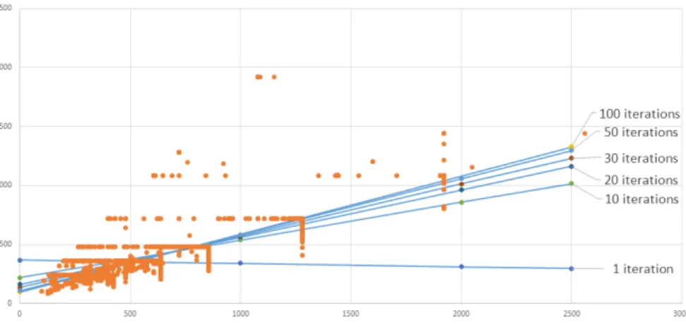
Linear regression in Spark is calculated using Stochastic Gradient Descent (SGD). In optimization phase it was decided to only set intercept calculation to true, set number of iterations to 100 and leave everything else to be optimized by Spark. The decision was made to get a more accurate result so it can be compared to SQL results on same data. Without setting intercept and number of iterations, Spark predicted values that were far from SQL predictions. Figure 5 illustrates how precision of predicted line increases with number of iterations. Number of it-erations is not always 100 as the algorithm stops automatically once corrections to slope and intercept are very small. It is worth noting that here optimization does not mean to achieve faster execution time but to get more accurate result. SGD optimization and other possible options are described in detail in [40]. Another thing to note is that SGD works best with small numbers. Therefore it was needed to normalize the data for MLlib regression function by dividing both width and height by 500 and take this into account when calculating values. 500 was selected as it produced the best result with initial data. Different number were tried and it was found 500 provided the best fit with low resolution and high resolution videos.

Figure 5: Converging of results in Spark MLlib linear regression by number of iterations

3.2.2 Simple Linear Regression in Spark SQL

Simple linear regression in Spark SQL does not require creation of new tables and therefore both HiveContext and SQLContext can be used here. Algorithm follows the same steps as described in 3.1.2.

In the first step of implementing simple linear regression in Spark SQL table schema is specified. Then an RDD is mapped from input data for columns that

(28)

hold this data. The RDD is then split into two: 80% for the calculation of regres-sion line and 20% for testing the outcome. Next step is to register a DataFrame and create a table for line calculation. For simple linear regression the SQL for calculating linear regression line is [38]:

SELECT ( (COUNT(∗) ∗ SUM( x∗y ) ) - (SUM( x ) ∗ SUM( y ) ) ) / ( (COUNT(∗) ∗ SUM( POW( x , 2 ) ) ) - POW(SUM( x ) , 2 ) ) a s i n t e r c e p t ,

AVG( y ) - ( (COUNT(∗) ∗ SUM( x∗y ) ) - (SUM( x ) ∗ SUM( y ) ) ) / ( (COUNT(∗) ∗

SUM(POW( x , 2 ) ) ) - POW(SUM( x ) , 2 ) ) ∗ AVG( x ) a s s l o p e

from Data

Final step that was not present in 3.1.2 is the testing part where values from test tables are compared to values predicted by linear regression model and mean error is calculated.

3.2.3 Simple Linear Regression in HiveQL

Implementing simple linear regression in HiveQL follows the step mentioned in 3.1.3. In the first step tables for training and test data are created, then input data is loaded to tables and finally exactly the same SQL query as in Spark SQL is run on created tables. Implementation of HiveQL differs from Spark SQL’s implementation as in HiveQL it is not possible to easily achieve the 80-20 input file split. The framework offers functions to partition table into buckets but this does not achieve 80-20 split in a reasonable number of queries. HiveQL also has a function to select a percentage of table but it is hard to make sure that two selections by percentage do not contain common rows. For HiveQL the input files were split beforehand to allow HiveQL’s query to be the same as in Spark SQL in order to keep run times for the two SQL-like frameworks comparable.

3.3

Multinomial Naive Bayes Classifier

Multinomial naive Bayes classifier is a multiclass classifier that assumes con-ditional independence between features - all features are independent from each other and can be looked at separately [41]. It is used to divide data into classes by comparing bayesian probabilities of features given class.

In the hearth of naive Bayes classifier is the Bayes theorem which uses prior events to calculate conditional probability of event under review: First thing in understanding Bayes theorem is conditional probability. To calculate probability of event Y =yi given event X =xk is true [?]:

P(X =xk|Y =yi) =

P(X =xk & Y =yi)

(29)

Bayes theorem [42]:

P(Y =yi|X =xk) =

P(X =xk|Y =Yi)P(Y =yi) P

yP(X =xk|Y =yj)P(Y =yj)

Naive Bayes classifier assumes that all features are conditionally independent. Conditional independence is when given that event Z occurs then if Y occurs or not does not provide any information on the likelihood of X occurring [43]. Mathematically [42]:

(∀i, j, k)P(X =xi|Y =yj, Z =zk) = P(X =xi|Z =zk)

Math behind Naive Bayes classifier is explained by T.Mithcell [42]. Naive Bayes classifier assumes that features are conditionally independent and by that greatly simplifies the representation and calculation of probabilities. Naive Bayes classifier assumes that in P(Y|X) where X = {x1, x2...xn}every xi is conditionally indepen-dent of every other xk given Y and also independent of every other subset of xk given Y. When X ={x1, x2} [42]:

P(X|Y) =P(x1, x2|Y) =P(x1|x2, Y)P(x2|Y) = P(x1|Y)P(x2|Y)

When X contains n attributes that are conditionally independent [42]:

P(x1...xn|Y) = n Y

i=1

P(xi|Y)

Bayes classifier uses the following formula to look for the most probable class C using conditionally independent features x1, x2, ..., xn [42]:

C =argmax( P(Y =Ck) Q iP(xi|Y =Ck) P jP(Y =Cj) Q iP(xi|Y =Cj) )

as the denominator does not depend on Ck the formula can be simplified to the following

C =argmax(P(Y =Ck) Y

i

P(xi|Y =Ck))

When working with small probabilities logarithm of probability will provide an-swers that can be more easily compared. Logarithm of probability also turns product into sum: log (x∗y) = logx+ logy . Sum is less CPU intensive than product and therefore accelerates calculating probabilities. Naive Bayes classifier expressed in logarithmic space:

C =argmax(logP(Y =Ck) + X

i=1

(30)

3.3.1 Multinomial Naive Bayes in Spark MLlib

First steps in implementing multinomial naive Bayes classifier from Spark ML-lib [41] are the same as described in 3.1.1. In mapping phase a new RDD is created that contains class and its features. The RDD is split in two for training and testing following the 80-20 split also used in linear regression. The training RDD is then used to train a Naive Bayes model which can be used to classify data according to features. Final step is the evaluation of data where model is used to predict classes in test RDD. Accuracy of model is calculated by comparing what was class predicted classes to what was the actual class.

3.3.2 Multinomial Naive Bayes in Spark SQL

Multinomial naive Bayes requires creation of many tables and therefore only HiveContext can be used here. In general it follows the same steps that were described in 3.1.2 with the addition of testing. In mapping phase features and classes are extracted from input file and schema is specified. This is followed by creation of RDD that is split 80-20 for training and testing. Next an SQL query is ran to create a table which holds data about features and classes. After this model is created by calculating the probabilities for every feature and class present in training data. Last step here is testing where model is used to predict classes on test data and accuracy of model is calculated.

SQL used for multinomial naive Bayes:

CREATE TABLE f c o e f s AS

SELECT f e a t u r e 1 , c l a s s , l o g ( ( f e a t u r e c o u n t + 0 . 5 ) / c l a s s c o u n t ) AS

f 1 c o e f , l o g ( ( c l a s s c o u n t + 0 . 5 ) / t o t a l ) AS c c o e f

FROM

(SELECT f e a t u r e 1 , c l a s s , v a l u e AS f e a t u r e c o u n t , SUM(v a l u e) OVER (PARTITION BY c l a s s ) AS c l a s s c o u n t , SUM(v a l u e) o v e r ( ) t o t a l

FROM

(SELECT f e a t u r e 1 , SUM( 1 ) AS v a l u e , c l a s s FROM d a t a GROUP BY

f e a t u r e 1 , c l a s s ) a ) b CREATE TABLE f 2 c o e f s AS SELECT f e a t u r e 2 , c l a s s , l o g ( ( f e a t u r e c o u n t + 0 . 5 ) / c l a s s c o u n t ) AS f 2 c o e f FROM (SELECT f e a t u r e 2 , c l a s s , v a l u e AS f e a t u r e c o u n t ,SUM(v a l u e) o v e r (PARTITION BY c l a s s ) AS c l a s s c o u n t FROM

(SELECT f e a t u r e 2 , SUM( 1 ) AS v a l u e , c l a s s FROM d a t a GROUP BY

f e a t u r e 2 , c l a s s ) a ) b

(31)

SELECT uid , t . f e a t u r e 1 , t . f e a t u r e 2 , t . c l a s s AS a c t u a l , a . c l a s s AS p r e d i c t i o n , f 1 c o e f+c c o e f+f 2 c o e f AS s c o r e FROM t e s t d a t a t INNER JOIN (SELECT f e a t u r e 1 , c l a s s , f 1 c o e f , c c o e f from f c o e f s ) a ON t . f e a t u r e 1 = a . f e a t u r e 1 INNER JOIN (SELECT f e a t u r e 2 , c l a s s , f 2 c o e f FROM f 2 c o e f s ) b ON t . f e a t u r e 2 = b . f e a t u r e 2 AND a . c l a s s = b . c l a s s

SELECT c o r r e c t /COUNT(∗) AS a c c u r a c y FROM t e s t d a t a

LEFT JOIN

(SELECT SUM( IF ( a c t u a l = p r e d i c t i o n , 1 , 0 ) ) c o r r e c t

FROM

(SELECT a c t u a l , p r e d i c t i o n , s c o r e , MAX( s c o r e ) OVER (PARTITION

BY u i d ) AS maxscore FROM t e s t s c o r e s ) a WHERE s c o r e = maxscore ) b

ON 1=1

GROUP BY c o r r e c t

3.3.3 Multinomial Naive Bayes in HiveQL

Implementing multinomial naive Bayes classifier in HiveQL follows the step mentioned in 3.1.3 . In the first step tables for training and test data are created, then input data is loaded into tables and finally exactly the same SQL query as in Spark SQL is run on created tables. Multinomial naive Bayes implementation also requires splitting input file to test and training data but to keep Spark SQL and HiveQL comparable the data was split beforehand.

(32)

4

Evaluation

In this chapter results of running the algorithms in Spark, Spark SQL and HiveQL are described. Algorithms were run using data sets of different sizes and number of executors was also modified. This thesis will also look at how well algorithms in Spark SQL and Spark MLlib scale, scaling of HiveQL is not looked into as it will always use as much resources as depending on how much is necessary and how much is given. It is possible to check how well Hive works depending on different number of CPU cores given to it but this requires reconfiguration of cluster between tests and it is too costly. Scaling of other two frameworks can be easily compared because number of CPU cores can be specified during execution

4.1

Cluster and Input Data

Algorithms were run in University of Tartu Mobile & Cloud Laboratory’s Cloudera Distribution Including Apache Hadoop - CDH 5.6.0 - cluster. It is a two machine cluster that is made up of two HP ProLiant DL180 G6 servers. Both servers have the same specifications:

• 2 CPUs: 4 core Xeon E5606

• RAM: 32 GB

• storage: 2 * 2 TB hard disks

• operating system: Ubuntu 12.04.1 LTS 64 bit

CPUs run on hyper threading - operation system assigns two addresses for each physical processor. This improves parallelization and means that operating system can use eight cores per processor when it has four physical cores.

CDH is running on four virtual machines: one master and three workers. Every machine shares the same configuration:

• CPU: 4 virtual CPUs acting as Intel T770 @ 2.40GHz

• RAM: 12 GB

• storage: 36 GB root disk + 200 GB storage disk

In total Cloudera has 16 CPU cores but only 8 can be used for YARN clusters: master is used for YARN, Cloudera uses one core per worker and YARN uses one core for driver.

Initial data for algorithms was downloaded from UCI Machine Learning Repos-itory [44] and bigger datasets were generated using limits identified from initial

(33)

dataset. Results obtained by running the algorithms on initial dataset is also described. Bigger data sets were generated to see how frameworks handle differ-ent amounts of data. Number of executors was also modified to see how scalable execution of algorithms is and how well parallelization is handled. Number of ex-ecutors (YARN clusters) was set to 1, 2, 4 and 8. With every generated dataset and number of worker nodes three tests were run, average run time from three tests is shown as run time.

Spark and Spark SQL were run in CDH using command line arguments. A script was used to start every algorithm with every dataset size and every number of executors three times. Results were taken from CDH Spark history server that displays run time when algorithm finishes execution. Using results from running the algorithms on biggest dataset parallel efficiency was also calculated [45]:

E(p) = T(n,1)

p∗T(n, p)

where T(n,1) is algorithm run time with one executor, T(n,p) is algorithm run time with p executors and p is the number of executors.

HiveQL was run in Cloudera Hue web application that allows access to CDH. Hue behaved differently than CDH using command line arguments. When execut-ing multiple SQL-s together Hue stopped between two queries for 7 - 15 minutes. That does not affect correlation results but when calculating run time for linear regression and naive Bayes classifier this was not taken into account. Results dis-played in this chapter for linear regression and naive Bayes classifier in HiveQL are sums jobs executed with the query. Hue did not present table creation times, these are not present in results.

4.2

Pearson’s Correlation Results

Initial data for running Pearson’s Correlation was downloaded from UCI Ma-chine Learning Repository[44]. Data set chosen for this algorithm was the Online Video Characteristics and Transcoding Time Dataset [46]. Original data set is a tsv file that contains 168 280 rows and 11 columns. Using this data set limits for new columns were identified and bigger datasets generated with 1, 3, 5 and 10 mil-lion rows to better understand how algorithms scale and handle bigger datasets. For correlation it was decided to use columns that contain video width and height to find if there is a correlation between these two values. With initial data all algorithms found the correlation to be 0.92 that shows strong linear correlation.

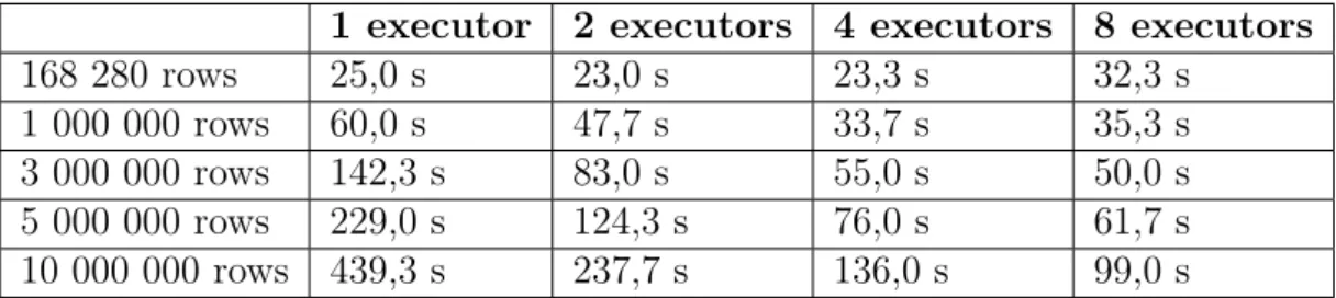
4.2.1 Pearson’s Correlation in Spark MLlib

(34)

1 executor 2 executors 4 executors 8 executors 168 280 rows 25,0 s 23,0 s 23,3 s 32,3 s 1 000 000 rows 60,0 s 47,7 s 33,7 s 35,3 s 3 000 000 rows 142,3 s 83,0 s 55,0 s 50,0 s 5 000 000 rows 229,0 s 124,3 s 76,0 s 61,7 s 10 000 000 rows 439,3 s 237,7 s 136,0 s 99,0 s

Table 2: Pearson’s Correlation in Spark MLlib

From the table it can be seen that run time grows as input data size grows. It also shows that with additional executors execution time decreases. With original dataset and 1 000 000 row dataset 8 executors is slightly slower that 4 executors but with bigger datasets more executors gives better performance. This means that the implementation of Pearson’s correlation in Spark MLlib is scalable and adding additional executors decreases run time. Parallel efficiency with 10 000 000 rows going from one executor to eight was 55,51%.

Implementation of Pearson’s correlation from Spark MLlib was straightforward and did not require any optimization. Only thing to do for a programmer in implementing the algorithm is to map data from input file to RDD and then split the RDD. This means that a programmer not familiar with Spark still has to learn what are RDD-s and how to use the map function.

4.2.2 Pearson’s Correlation in Spark SQL

Results of running Pearson’s Correlation in Spark SQL using HiveContext are shown in table 3 and results when using SQLContext are shown in 4.

1 executor 2 executors 4 executors 8 executors

168 280 rows 38,7 s 36,0 s 31,0 s 39,0 s

1 000 000 rows 53,3 s 39,0 s 33,3 s 36,0 s

3 000 000 rows 112,0 s 69,0 s 49,3 s 46,3 s

5 000 000 rows 170,3 s 99,3 s 64,7 s 56,0 s

10 000 000 rows 319,0 s 172,3 s 106 s 85,3 s

Table 3: Pearson’s correlation in Spark SQL HiveContext

Both tables show similar numbers and from this it can be concluded that in implementing Pearson’s correlation it does not matter which Context to use. The results here also show that with initial data Spark SQL was slightly slower when compared to Spark MLlib’s implementation. However, starting from 1 000 000 rows Spark SQL’s run time started performing better with 2 executors and was

(35)

1 executor 2 executors 4 executors 8 executors 168 280 rows 38,0 s 35,0 s 30,7 s 38,3 s 1 000 000 rows 53,0 s 33,7 s 33,0 s 35,3 s 3 000 000 rows 113,3 s 68,3 s 48,0 s 48,7 s 5 000 000 rows 169,3 s 98,3 s 63,3 s 55,7 s 10 000 000 rows 320,0 s 171,7 s 103,7 s 87,3 s

Table 4: Pearson’s correlation in Spark SQL SQLContext

2.4 times faster with 5 000 000 input rows and 2 executors. There aren’t many differences with 8 executors, excluding 5 000 000 rows input file where Spark SQL was 1.7 times faster. Parallel efficiency with 10 000 000 rows going from one executor to 8 was 46,75% for HiveContext and 45,82% for SQLContext.

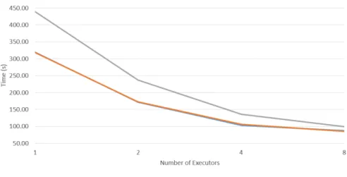
Figure 6 shows the how additional executors decrease run time. Table also shows how similar SQLContext and HiveContext run times were - their lines are almost the same.

Figure 6: Framework Speed Up Comparison in Pearson’s Correlation using 10 000 000 row dataset

Implementation of Pearson’s correlation in Spark SQL required only selecting data from table and then performing calculations on selected data. This could be done by any programmer familiar with SQL. The obvious difficulties here are reading data from input file that is not in json format as then programmer has to manually specify table schema and map data from file to RDD. Event though Spark SQL is SQL-like it still requires some low level programming that is not

(36)

present when only working with SQL. Running SQLs on DataFrame can be done by any programmer familiar with SQL and requires no knowledge or lower level programming.

4.2.3 Pearson’s Correlation in HiveQL

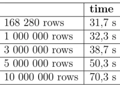
Results of running Pearson’s correlation in HiveQL are shown in table 5:

time 168 280 rows 31,7 s 1 000 000 rows 32,3 s 3 000 000 rows 38,7 s 5 000 000 rows 50,3 s 10 000 000 rows 70,3 s

Table 5: Pearson’s correlation in HiveQL

The most interesting thing to note here is that HiveQL performed on par with Spark SQL and outperformed algorithm from Spark MLlib. Input table creation times are not present in HiveQL results but for largest dataset it was 1.4 seconds, faster than 29 seconds - difference between HiveQL and Spark MLlib using biggest dataset and maximum number of executors.

Implementation of Pearson’s correlation in HiveQL requires only knowledge of SQL. Input data is read from file using SQL and then SQL query is ran on created table. There is no need to map data from file or perform optimizations that were present in Spark MLlib. One issue when implementing this algorithm was that HiveQL does not support the function MEAN() but as it is just a different name for AVG() this did not stop the implementation.

4.3

Simple Linear Regression Results

Initial data for running simple linear regression is the same Online Video Char-acteristics and Transcoding Time Dataset used with correlation. Bigger generated datasets with 1, 3 and 5 million rows that were used with Pearson’s correlation algorithm are also used here.

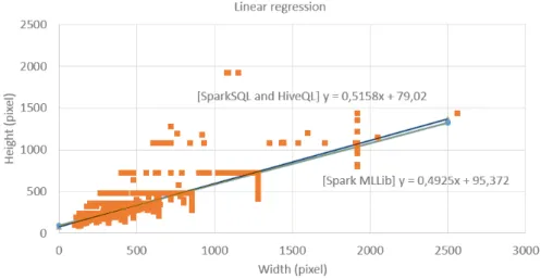
Results of running linear regression algorithm on original data is visualized are figure 7. HiveQL and Spark SQL produced exactly the same result, result from Spark MLlib algorithm is slightly different. The difference comes from how algorithms calculate the result - SQL frameworks used a well-defined formula that produced one result each time it was run. Spark MLlib algorithm used SGD and therefore the results varied between runs but only by 10−13 _{for both slope and}

(37)

Figure 7: Vizualization of linearregression results

4.3.1 Simple Linear Regression in Spark MLlib

Results of running simple linear regression in Spark are shown in the table 6.

168 280 rows 56,0 s 48,3 s 47,7 s 58,3 s

1 000 000 rows 94,0 s 71,3 s 62,7 s 66,0 s

3 000 000 rows 199,3 s 127,0 s 91,0 s 83,7 s

5 000 000 rows 331,0 s 178,3 s 119,7 s 99,3 s

Table 6: Spark Linear Regression

From the table it can be seen that run time grows as input data size grows. It also shows that with additional executors execution time decreases with one exception. Adding additional executors to original dataset actually increased run time. Difference in run time between different number of executors in 1, 3 and 5 million row datasets show that with bigger datasets this algorithm is scalable. For 5 000 000 row dataset the scaling efficiency between 1 executor and 8 executors was 41,6%.

As linear regression is already implemented in Spark MLlib then implementing this is relatively easy. However, the algorithm does not calculate the line in a straight forward way but required some optimization. For accurate results number of iterations had to be set and it was also necessary to divide values by 500. This was required because the algorithm used SGDs that are optimized for working with small numbers. This highlights the issue that Spark MLlib’s linear regression requires knowledge about the internal workings of the implementation.

(38)

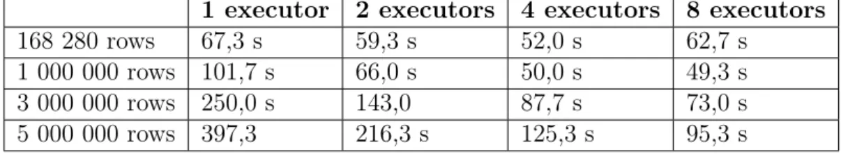
4.3.2 Simple Linear Regression in Spark SQL

Results of running linear regression are shown in the two tables below. Results when using HiveContext are shown in table 7 and results using SQLContext are shown in table 8.

168 280 rows 67,3 s 59,3 s 52,0 s 62,7 s

1 000 000 rows 101,7 s 66,0 s 50,0 s 49,3 s

3 000 000 rows 250,0 s 143,0 87,7 s 73,0 s

5 000 000 rows 397,3 216,3 s 125,3 s 95,3 s

Table 7: Linear Regression in Spark SQL using HiveContext

168 280 rows 68,0 s 61,3 s 52,3 s 62,0 s

1 000 000 rows 102,7 s 66,0 s 50,7 s 50,3 s

3 000 000 rows 250,3 s 140,0 s 91,0 s 74,0 s

5 000 000 rows 394,7 215,3 s 126,3 s 96,7s

Table 8: Linear Regression in Spark SQL using SQLContext

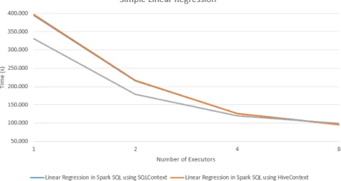
Both tables show similar numbers and from this it can be concluded that in simple linear regression’s implementation in Spark SQL it does not matter which Context to use for SQL. The tables also show that with 1 and 2 executors Spark SQL was slower than Spark, execution times were similar with 4 executors and 8 executors. This combined with the fact that run times decrease faster with every additional executor shows that with this algorithm Spark SQL scales better than Spark MLlib’s implementation, this is illustrated in figure 8. For 5 million row input file the scaling efficiency was 51,0% for HiveContext and 52,1% SQLContext. Implementation of linear regression in Spark SQL only required selecting data from table. Writing the SQL is doable for a programmer that has knowledge about SQL. The additional step here, when compared with implementation of Pearon’s correlation, was testing where created model was compared to test data and this required splitting up input data for test and training data. This, combined with the fact that reading data from text file requires the specification of schema and mapping the data to schema, means that programmer also has to learn what are RDDs and how to map data from input file. When this is done, everything else is done by using SQL. One issue encountered here is that in Spark SQL variables cannot be saved using SQL. The algorithm had to do some calculations twice and one calculation - count(*) - four times, saving result to a variable could help here.

(39)

Figure 8: Framework Speed Up Comparison in Simple Linear Regression using 3 000 000 row dataset

The thesis did not check the internal workings of Spark SQL to see how well it is optimized. Future work is needed here to investigate how this is handled to see if using variables could help speed up the process.

4.3.3 Simple Linear Regression in HiveQL

Results of running simple linear regression in HiveQL are shown in the table 9. time 168 280 rows 107,7 s 1 000 000 rows 109,0 s 3 000 000 rows 122,3 s 5 000 000 rows 132,3 s Table 9: Linear regression in HiveQL

From the table it can be seen that even though size of dataset increased more than five times run times remained relatively the same. Run times are slower than run times in Spark SQL and Spark MLlib with 8 executors for every input size.

HiveQL required the processing of files beforehand while Spark MLlib version and Spark SQL version were able to split input file into test and train easily. It was decided to split files beforehand with a Python script as HiveQL lacked the

(40)

function to split file randomly using sizes in percentages. There was the option to split files into buckets and then select data from only several buckets but that does not allow the 80-20 split that is possible in Spark SQL and Spark. Hive also had the option to randomly select 80% and 20% of data but there was no way to make sure that these two splits didn’t share common data.

Implementation of linear regression in HiveQL was only using SQL. There was no need for additional lower level programming and therefore every programmer who has knowledge about SQL can implement this algorithms. All the issues encountered with this algorithm were related to Hue but there were no issues with writing SQL. HiveQL does also not support storing variables. This thesis did not look into the inner workings of HiveQL and future work is required here to see how well HiveQL optimizes queries where same SQL calculations are used many times.

4.4

Multinomial Naive Bayes Classifier Results

Initial data used for multinomial naive Bayes is Covertype Data Set [47] from UCI Machine Learning Repository [44]. Covertype Data Set contains 581 012 rows and 13 attributes. For multinomial naive Bayes it was decided to use two features to classify cover type. The features selected were elevation and aspect. From intintal dataset bigger datasets were gener