Abstract—There is biological evidence to prove information is coded through precise timing of spikes in the brain. However, training a population of spiking neurons in a multilayer network to fire at multiple precise times remains a challenging task. Delay learning and the effect of a delay on weight learning in a spiking neural network has not been investigated thoroughly. This research proposes a novel biologically plausible supervised learning algorithm for learning precisely timed multiple spikes in a multilayer spiking neural networks. Based on the spike timing dependent plasticity (STDP) learning rule, the proposed learning method trains a spiking neural network through the synergy between weight and delay learning. The weights of the hidden and output neurons are adjusted in parallel. The proposed learning method captures the contribution of synaptic delays to the learning of synaptic weights. Interaction between different layers of the network is realised through biofeedback signals sent by the output neurons. The trained spiking neural network is used for classification of spatiotemporal input patterns. The proposed learning method also trains the spiking network not to fire spikes at undesired times which contribute to misclassification. Experimental evaluation on benchmark datasets from the UCI machine learning repository shows that the proposed method has comparable results with classical rate based methods such as Deep Belief Network and the Autoencoder models. Moreover, the proposed method can achieve higher classification accuracies than single layer and a similar multilayer spiking neural network.
Index Terms—Multilayer Neural Network, Spiking Neural Network, Supervised Learning, Synaptic Delay.
I. INTRODUCTION
PIKE timing dependent plasticity (STDP) plays a prominent role in learning in biological neurons, and it represents one form of synaptic plasticity which underpins synaptic weight changes based on the precise times of pre and postsynaptic spikes [1]. STDP highlights the important role of precise spike times in information processing in the brain [2]. Additionally, the rapid sensory processing observed in the visual, auditory and olfactory systems supports the assumption
This work was supported by the Ulster University’s Vice Chancellor’s Research Scholarship Scheme.
A. Taherkhani is with the the Computational Neuroscience and Cognitive Robotics Laboratory at Nottingham Trent University, Nottingham, UK. (e-mail: [email protected])
that information is encoded in the precise timing of the spikes [3]-[5]. Moreover, using precise timing of spikes results in a higher information encoding capacity compared with rate based coding [6], and it can also convey the information related to rate of spikes in a multi-spike coding scheme [2]. Furthermore, as neural activity is metabolically expensive, the high number of spikes involved in rate coding scheme demands a significant amount of energy and resources [7], [8]. Despite the existing evidence supporting information encoding using the precise timing of spikes, the exact neuronal mechanisms that underlie learning to fire at precise times is still not clear and remains one of the challenging problems in the field of spiking neural networks [2], [9]-[11].
In this research, a novel supervised learning algorithm inspired by STDP is proposed to train a spiking neural network (SNN) to fire multiple spikes at precise desired times. Local synaptic biochemical events, produced by incoming spikes, are used to adjust weights and delays appropriately. Additionally, neurons in the output and hidden layers interact with each other through a biofeedback signal sent by the output neurons to train the network. The main novelty of the proposed method consists in (1) capturing the effect of synaptic delays on the learning of neuronal connection weights in an SNN, which has not been considered in previous works, and (2) learning the spiking network synaptic delays. In addition, the proposed approach introduces an additional training mechanism to prevent the occurrence of undesired spikes which contribute to misclassification of spatio-temporal input patterns. The proposed approach is validated using benchmark classification datasets and is compared against both spiking and rate-based neural models including state-of-the-art deep learning and autoencoder models. The experimental results show an improvement in learning accuracy over existing competitive spiking neural network architectures and comparable performance to state-of-the-art rate-based neural models.
The remainder of the paper is structured as follows. A brief review of background and related work on SNNs is presented in section II. Section III introduces the proposed method in
A. Belatreche is with the Department of Computer and Information Sciences, Northumbria University, Newcastle upon Tyne, NE1 8ST. (e-mail: [email protected]).
Y. Li is with the School of Computer Science and Informatics, Cardiff University, U.K. (e-mail: [email protected]).
L. P. Maguire is with the Faculty of Computing and Engineering, Ulster University, Derry BT48 7JL, U.K. (e-mail: [email protected]).
A Supervised Learning Algorithm for Learning
Precise Timing of Multiple Spikes in Multilayer
Spiking Neural Networks
Aboozar Taherkhani, Ammar Belatreche, Yuhua Li, and Liam P. Maguire
detail. The simulation results are then provided in section IV. Finally, section V concludes the paper.
II. BACKGROUND AND RELATED WORK
Different artificial neural networks (ANNs) have been devised based on the working principle of their biological counterparts. McCulloch and Pitts (1943) developed the first artificial neural network where the neuron model is a logic unit which can be in an active or inactive (binary) mode depending on the weighted sum of their binary inputs. Later, a continuous transfer function (e.g., sigmoid function) is applied to the weighted sum of continuous inputs to generate continuous output [12]. The continuous values represent the biological neuron spiking rates. ANNs are inspired by the biological nervous system and are successfully used in various applications. However, their high abstraction compared to their biological counterparts [13] and their inability to capture the complex temporal dynamics of biological neurons have resulted in a new area of ANNs where the focus is placed on more biologically plausible neuronal models known as Spiking Neural Networks (SNNs). Thanks to their ability to capture the rich dynamics of biological neurons and to represent and integrate different information dimensions such as time, frequency, phase etc., SNNs offer a promising computing paradigm and are potentially capable of modelling complex information processing in the brain [14]-[20].
In 1952, Hodgkin and Huxley [16] built a four dimensional (4D) detailed conductance-based neuron model which can reproduce electrophysiological measurements to a high degree of accuracy. However, because of its intrinsic computational complexity this model has a high computational cost. For this reason, simple phenomenological spiking neuron models are employed for simulating large scale SNNs [15]. The Leaky Integrate-and-Fire (LIF) model is a popular 1D spiking neural model with low computational cost, but it offers relatively poor biological plausibility compared with the Hodgkin and Huxley model. Simple phenomenological spiking neuron models with low computational cost are highly popular for studies of neural coding, memory, and network dynamics [12].
The first supervised learning algorithms for multilayer SNNs using the precise timing of spikes could train only a single spike for each neuron. Bohte et. al. [21] proposed the multilayer SNN called SpikeProp (inspired by the classical back propagation algorithm) as one of the first supervised learning methods for feedforward multilayer SNNs. Back-propagation with momentum [22], QuickProp [22], resilient propagation (RProp) [22], [23], and the SpikeProp based on adaptive learning rate [24] were proposed to improve the performance of SpikeProp. In all these methods, neurons in the input, output and hidden layers can only fire a single spike.
Despite the capability of a single-spike learning method, single-spike coding schemes limit the diversity and capacity of information transmission in a network of spiking neurons (SNs). In contrast, multiple spikes significantly increase the richness of the neural information representation [25], [26]. Additionally, training a neuron to fire multiple spikes is more biologically plausible compared to single-spike learning methods [27], [28]. Temporal encoding through multiple spikes
transfers important information which cannot be expressed by a single spike coding scheme or a rate coding scheme. Although the exact mechanism of information coding in the brain is not clear, biological evidence shows that multiple spikes have a pivotal role in the brain. For instance, mapping between spatiotemporal spiking sensory inputs composed of spike trains to precise timing of spikes is an essential characteristic of neuronal circuits of the zebra finch brain to execute well-timed motor sequences [29]. In the mixed approaches proposed in [30] and [31], it is suggested that using both spike timing and spike rate increases processing speed. These methods use a combination of both correlated and uncorrelated spiking signals. So, there is useful information in the spike rate that cannot be captured by the precise timing of single spikes. Encoding information in the precise timing of multiple spikes which are used in this research not only can capture the information in the spike rate but also can capture the information in inter spike intervals.
Pfister et al. [32] designed a supervised learning algorithm for a single SN which updates synaptic weights to increase the likelihood of postsynaptic firing at several desired times. The algorithm is designed to train only a single neuron; however, it can train the neuron to fire multiple desired spikes. ReSuMe [25], SPAN (Spike Pattern Association Neuron) [33], PBSNLR (Perceptron-Based Spiking Neuron Learning Rule) [34], BPSL (Biologically Plausible Supervised Learning Method) [35], and EMPD (Efficient Membrane Potential Driven supervised learning method) [36] are other examples of learning methods that can train a single neuron to fire multiple desired spikes. Multi-spike learning methods focus on a single neuron or a single-layer of neurons. It is difficult to design a multilayer SNN to fire multiple desired spikes because the complexity of the learning task is increased [27], [37]. In this situation, the learning algorithm should control several neurons to generate different desired spikes. However, a real biological nervous system is composed of a large number of interconnected neurons [27], [28], [37].
A multilayer neural network has a higher information processing ability than a single layer of neurons. Sporea et al. [28] have shown that a multilayer SNN can perform a nonlinearly separable logical operation; however, the task cannot be accomplished without the hidden layer neurons.
Booij et al. [38] and Ghosh-Dastidar et al. [37] extended the multilayer SpikeProp [21] to allow each neuron in the input and hidden layers to fire multiple spikes. However, each output neuron can fire only a single spike. Xu et al. [27] proposed the first supervised learning method based on the classical error backpropagation method that can train all the neurons in a multilayer SNN to fire multiple spikes. Gradient learning methods suffer from various known problems which can lead to learning failure such as sudden jumps (called surge) or discontinuities in the error function [24]. The problem becomes more severe when the output neurons are trained to fire more than a single spike. Additionally, the construction of an error function becomes difficult when multiple desired spikes should be learned as the number of actual output spikes may differ from the number of desired spikes in each learning epoch [27].
After investigation of the gradient based methods in [23], [39], [40], it is concluded that the application of STDP is worth further investigation to implement a more biologically plausible learning algorithm for multilayer SNNs [37].
Sporea et al. [28] have used STDP and anti-STDP to devise the first biologically plausible supervised learning algorithm for classification of real world data by a multilayer SNN in which each neuron in the input, hidden and output layers can fire multiple spikes. The authors did not consider the spikes fired by hidden neurons when training the hidden neurons parameters. However, in a biological neuron, STDP usually works on the pre- and postsynaptic spikes of the neuron. Additionally, the output spikes of the hidden neurons have significant effects on a training task in a multilayer SNN. Another drawback of this method [28] is that it has used the same learning adjustment method for inhibitory and excitatory neurons in hidden layers. However, inhibitory and excitatory neurons have different effects in a network by generating positive and negative PSP (postsynaptic potential). In this research, a method is proposed to use spikes fired by hidden neurons during learning, and excitatory and inhibitory neurons are trained appropriately.
Delays of spike propagation are an important characteristic of real biological neural systems, and they have a significant effect on the information processing ability of the nervous system [18], [41], [42]. In EDL [43], an extended delay learning based remote supervised method for SNs, and DL-ReSuMe [41], a Delay Learning based Remote Supervised Method for SNs, investigated the viability of adjusting the neuron synaptic weights and delays for training a single SN to map a given spatiotemporal input pattern into a desired output spike train. STDP and anti-STDP were used to adjust the synaptic weights and a delay shift approach was used to adjust their delays. It is worth noting that constant synaptic delays have been employed in [28] , hence neglecting the effect of a synaptic delay between a hidden neuron and an output neuron on the weight adjustment of the hidden neuron. It trains the hidden neuron to fire at the time of an output desired spike. However, the generated spike is shifted by the network synaptic delay and causes an error in the firing time of the output neuron. SpikeProp and its related gradient based methods [21], [23], [37] have taken into account the effect of a delay between a hidden neuron and an output neuron on the input weight adjustment of the hidden neurons. However, the use of multiple connections with different delays after a hidden neuron causes each of the different delays to affect the adjustment of the hidden neuron weights in different and opposite directions. Because, different errors are propagated from an output neuron to a hidden neuron corresponding to the different sub-connections between the two neurons. The different errors force the hidden neuron to fire at different times depending on the different delays related to the multiple connections, and it disturbs the learning procedure. This might be one reason for the huge sudden rise in learning error of SpikeProp as reported in [24].
In this research, a learning algorithm is proposed to train both weights and delays of a multilayer SNN to fire multiple desired spikes. In the proposed method, each neuron at input, hidden and output layers can fire multiple spikes. Supervised training
of spiking neurons which fire multiple spikes in a multilayer spiking neural network remains a challenge. Furthermore, the proposed approach trains the synaptic delays in the multilayer SNN and also takes into the effect of delays on weight adjustments which is not considered in [21]-[24], [28]. In the proposed method, the effect of the delays between a hidden neuron and an output neuron is considered during weight adjustments of the hidden neuron. Additionally, the proposed method trains the weights of the hidden neurons by using the spikes fired by hidden neurons during STDP and anti-STDP, which results in a more biologically plausible and a highly accurate learning. Moreover, different weight adjustment strategies are used to train excitatory and inhibitory hidden neurons based on the effect of the excitatory (positive) and inhibitory (negative) PSP (EPSP and IPSP) produced by the trained hidden neurons. In the following section the principle of the proposed method is described.
III. MATERIALS AND METHODS
The aim of the proposed supervised learning algorithm is to train a multilayer SNN to map spatiotemporal input patterns to their corresponding desired spike trains which implements a classification of the spatiotemporal input patterns. The network is composed of an input, a hidden and an output layer. An output neuron, called a readout neuron, is fully connected to the hidden neurons. A spatiotemporal input pattern is emitted by the neurons in the input layer. Each input neuron is randomly connected to a fraction number of hidden neurons as used in [18]. The Leaky Integrate and Fire (LIF) neuron model described in [41] is used. The proposed method trains the spiking network by adjusting the learning parameters of the hidden and output neurons in parallel.
A. Overview of the Proposed Learning Method
The proposed learning method aims to train the multilayer SNN to enable each readout (output) neuron to fire actual output spikes at desired times and to cancel out undesired output spikes. A remote supervising signal is considered for an output neuron similar to ReSuMe [25]. At the time of a desired spike where there aren’t any actual output spikes at the readout neuron, the network learning parameters are adjusted to increase the total PSP of the readout neuron to hit the threshold level and generate an actual output spike at the desired time by using biologically plausible local events. The output neuron does the following three activities in parallel at the desired spike time.
First, at the time of the desired spike the output neuron sends back an instruction signal (biofeedback) that shows the time of desired spike to the hidden neurons. After receiving the instruction signal, an excitatory hidden neuron potentiates its weights based on STDP to fire an output spike (hidden spike) at a specific time interval before the desired time. The specific time interval is equal to the delay related to the connection between the excitatory hidden neuron and the output neuron. The effect of the generated hidden spike (i.e. the PSP generated by the hidden spike) is shifted to the desired spike time after the related delay between the hidden neuron and the output neuron.
The potentiation of the excitatory hidden neuron weights is stopped when the hidden neuron firing rate reaches a certain value, because a biological neuron cannot fire with a limitless rate, and a refractory period will ensure an upper bound on the neuron firing rate. The excitatory hidden neuron weight potentiation at the time of a desired spike is also stopped when an actual spike is generated at the time of the desired spike by the output neuron. Additionally, the feedback triggers an inhibitory hidden neuron to try to remove its output spikes fired a specific time interval before the desired time by using the long-term depression (LTD) of anti-STDP. The time interval is equal to the delay between the inhibitory hidden neuron and the readout neuron. The hidden neuron output spikes before the time interval affects the PSP of the readout neuron at the desired time, i.e. the hidden spikes generate delayed PSPs at the desired time. The reduction of the inhibitory hidden spikes helps the readout neuron to increase its total PSP at the desired time to hit the threshold level.
Secondly, similar to ReSuMe [25] the output neuron potentiates its weights that have a spike shortly before the desired time based on STDP to increase its PSP at the desired time to fire.
The third activity at the time of a desired spike where there are not any actual output spikes of the readout neuron is the adjustment of delays of the readout neuron to increase the PSP of the readout neuron at the desired time, based on EDL [43]. All the above-mentioned activities are repeated at the time of other desired spikes in a multi spike coding scheme.
At the time of an undesired output spike of the readout neuron (i.e. where there is an actual output spike and there aren’t any desired spikes), the learning algorithm should reduce the total PSP of the readout neuron at the time of the undesired output spike to remove it by applying the following three processes in parallel. First the readout neuron sends a feedback to excitatory hidden neurons to instruct them to remove their output spikes. Each excitatory hidden neuron removes its spike fired at a precise time interval before the time of the undesired spike by using LTD based on anti-STDP and reduces its weights. The time interval for the hidden neuron is equal to the delay between the hidden neuron and the readout neuron. Consequently, the reduction of the excitatory hidden neuron weights can help the readout neuron to reduce its total PSP and to remove the undesired output spike. It is clear that the weight reduction should be applied to the excitatory neurons that have a number of output spikes. Therefore, the LTD is applied to the excitatory neurons when their firing rates are higher than a threshold rate. The threshold rate is set by trial and error. Additionally, the feedback triggers each inhibitory hidden neuron to potentiate its weights based on the long-term potentiation (LTP) of STDP. The weight potentiation increases inhibitory hidden spikes before a precise time interval (the time interval is equal to the delay between the hidden neuron and the readout neuron) before the undesired spike time to help the readout neuron to reduce its total PSP at the undesired output spike time. The second process is applied at the time of the undesired output spike and consists of a reduction of the readout neuron weights that have spikes at the undesired output spike
time or shortly before it by using anti-STDP similar to ReSuMe [25]. The third process reduces the readout neuron total PSP at the time of the undesired spike by adjusting the delays of the readout neuron based on EDL [43].
The hidden layer spikes play an important role in the generation of the network output spikes (both at desired and undesired times). Generated spikes by different hidden neurons cooperatively increase the PSP of the output neuron at a desired time and help it to fire at the desired time. Additionally, when the complexity of a learning task is increased by increasing the number of desired spikes and also by increasing the number of different training patterns for each class, it becomes difficult or impossible to train a single neuron to fire at all the desired times for all the training patterns. Different groups of hidden neurons can contribute in generating different desired spikes and cooperatively drive a readout neuron to fire at all the desired times for all the training patterns.
In the following sections, first the training rule of the output neurons are explained then the training of the hidden neurons weights is described in detail.
B. Training the Output Neurons
The weights and delays of each output neuron are trained by EDL as described in [43]. The delay adjustments in cooperation with the weight adjustments train an output neuron to increase its total PSP at a desired time to generate an actual output spike, and also the adjustments help the output neuron to reduce its PSP at undesired spike times and to remove undesired actual output spikes. The weights are trained by the following equation: 𝑑𝑤𝑜ℎ(𝑡) 𝑑𝑡 = [𝑠𝑜 𝑑(𝑡) − 𝑠 𝑜𝑎(𝑡)][𝑎 + ∫ 𝛹(𝑠)𝑠ℎ(𝑡 − 𝑑𝑜ℎ− 𝑠)𝑑𝑠 +∞ 0 ] (1) where 𝑤𝑜ℎ and 𝑑𝑜ℎ are the weight and delay related to the connection between the ℎ𝑡ℎ hidden neuron and the 𝑜𝑡ℎ output neuron, respectively. 𝑠𝑜𝑑(𝑡) and 𝑠𝑜𝑎(𝑡) are desired and actual output spike trains of the 𝑜𝑡ℎ output neuron respectively. 𝑠
ℎ(𝑡) is the spike train fired by ℎ𝑡ℎ hidden neuron. 𝑎 is a non-Hebbian parameter that can speed up the learning. 𝛹(𝑠) is a learning window similar to that of STDP and has an exponential function as described by equation (2).
𝛹(𝑠) = {𝐴e−𝑠/𝜏 , 𝑠 ≥ 0
0, 𝑠 < 0 (2)
where 𝜏 and 𝐴 are the exponential decay time constant and the amplitude of the learning window respectively.
𝑥𝑜ℎ(𝑡), a local variable called spike trace, is used to train the delay related to the synapse that connect ℎ𝑡ℎ excitatory hidden neuron to 𝑜𝑡ℎ output neuron. 𝑥
𝑜ℎ(𝑡) is governed by equation (3). 𝑥𝑜ℎ(𝑡) = { 𝐴e−(𝑡−𝑡ℎ𝑓−ɛ𝑜ℎ)/𝜏 , 𝑡 ℎ 𝑓 < 𝑡 < 𝑡ℎ𝑓+1 𝐴, 𝑡 = 𝑡ℎ 𝑓 (3)
where 𝑡ℎ𝑓 is the firing time of the 𝑓𝑡ℎ spike of the ℎ𝑡ℎ excitatory hidden neuron, 𝜏 is the time constant of the exponential function, ɛ𝑜ℎ is the delay between the ℎ𝑡ℎ excitatory hidden neuron and the 𝑜𝑡ℎ output neuron, and A is a constant value which are equal to their counterparts in (2). 𝑥𝑜ℎ(𝑡) is used to obtain appropriate value for delay adjustment. The adjustment
∆ɛ𝑜ℎ is calculated by (4) similar to EDL [43].
∆ɛ𝑜ℎ(𝑡) = { +∆𝑡𝑜𝑚(𝑡)(𝑥𝑜ℎ(𝑡) 𝑥⁄ 𝑜𝑚(𝑡))4, 𝑡 = 𝑡̂𝑜 𝑓 −∆𝑡𝑜𝑚(𝑡)(𝑥𝑜ℎ(𝑡) 𝑥⁄ 𝑜𝑚(𝑡))4, 𝑡 = 𝑡𝑜𝑓 0, Otherwise (4) where 𝑡̂𝑜 𝑓
is the time of the 𝑓𝑡ℎ desired spike and 𝑡 𝑜 𝑓
is the time of the 𝑓𝑡ℎ actual output spike of the 𝑜𝑡ℎ output neuron, 𝑥
𝑜𝑚(𝑡) is the maximum trace between the traces of the excitatory hidden neurons connected to the 𝑜𝑡ℎ output neuron at the current time 𝑡. 𝑥𝑜𝑚(t) is corresponding to the connection between the 𝑚𝑡ℎ excitatory hidden neuron (that has the closest spike before the current time t) and the 𝑜𝑡ℎ output neuron. ∆𝑡
𝑜𝑚 is a delay shift which is necessary to be added to the delay between the 𝑚𝑡ℎ excitatory hidden neuron and the 𝑜𝑡ℎ output neuron to bring the effect of the closest spike fired by 𝑚𝑡ℎ excitatory hidden neuron to the current time 𝑡. It is derived from (3) and calculated by (5).
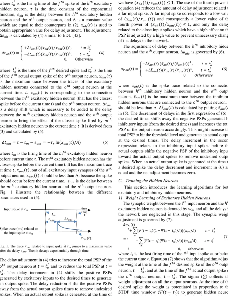
∆𝑡𝑜𝑚= 𝑡 − 𝑡𝑚− ɛ𝑜𝑚= −𝜏𝑥ln(𝑥𝑜𝑚(𝑡)/𝐴) (5) where 𝑡𝑚 is the firing time of the 𝑚𝑡ℎ excitatory hidden neuron before current time 𝑡. The 𝑚𝑡ℎ excitatory hidden neuron has the closest spike before the current time t. It has the maximum trace at time 𝑡, 𝑥𝑜𝑚(𝑡), out of all excitatory input synapses of the 𝑜𝑡ℎ output neuron. 𝑥𝑜𝑚(𝑡) should be less than A, because the spike should occur before the current time. ɛ𝑜𝑚 is the delay between the 𝑚𝑡ℎ excitatory hidden neuron and the 𝑜𝑡ℎ output neuron. Fig. 1 illustrate the relationship between the different parameters used in (5).
Fig. 1. The trace 𝑥𝑜𝑚 related to input spike at 𝑡𝑚 jumps to a maximum value
after the delay ɛ𝑜𝑚. Then it decays exponentially through time
.
The delay adjustment in (4) tries to increase the total PSP of the
𝑜𝑡ℎ output neuron at 𝑡 = 𝑡̂ 𝑜 𝑓
and to reduce the total PSP at 𝑡 = 𝑡𝑜
𝑓
. The delay increment in (4) shifts the positive PSPs generated by excitatory inputs to the desired times to generate an output spike. The delay reduction shifts the positive PSPs away from the actual output spikes times to remove undesired spikes. When an actual output spike is generated at the time of a desired spike the positive delay adjustment cancels out the negative delay adjustment and the delays are stabilized. In (4)
we have (𝑥𝑜ℎ(𝑡) 𝑥⁄ 𝑜𝑚(𝑡)) ≤ 1. The use of the fourth power in equation (4) reduces the amount of delay adjustment related to a far input spike. A far input spike corresponds to a low value of (𝑥𝑜ℎ(𝑡) 𝑥⁄ 𝑜𝑚(𝑡)) and consequently a lower value of the fourth power of (𝑥𝑜ℎ(𝑡) 𝑥⁄ 𝑜𝑚(𝑡)) ≤ 1, and only the delays related to the close input spikes which have a high effect on the PSP is adjusted by a high value to prevent unnecessary change of the delays in the network.
The adjustment of delay between the ℎ𝑡ℎ inhibitory hidden neuron and the 𝑜𝑡ℎ output neuron, ∆𝜇
𝑜ℎ, is governed by (6). ∆𝜇𝑜ℎ(𝑡) = { −∆𝑡̅𝑜𝑚(𝑡) (𝑥̅𝑜ℎ(𝑡) (𝑥̅⁄ 𝑜𝑚(𝑡))4, 𝑡 = 𝑡̂𝑜 𝑓 +∆𝑡̅𝑜𝑚(𝑡)(𝑥̅𝑜ℎ(𝑡) 𝑥̅⁄ 𝑜𝑚(𝑡))4, 𝑡 = 𝑡𝑜 𝑓 0, 𝑂𝑡ℎ𝑒𝑟𝑤𝑖𝑠𝑒 (6)
where 𝑥̅𝑜ℎ(𝑡) is the spike trace related to the connection between ℎ𝑡ℎ inhibitory hidden neuron and the 𝑜𝑡ℎ output neuron. 𝑥̅𝑜𝑚(𝑡) is the maximum trace between the inhibitory hidden neurons that are connected to the 𝑜𝑡ℎ output neuron. It should be less than A. ∆𝑡̅𝑜𝑚(𝑡) is calculated by putting 𝑥̅𝑜𝑚(𝑡) in (5). The decrement of delays in the first expression of (6) at the desired times shifts away the negative PSPs generated by inhibitory inputs (from the desired times) and increases the total PSP of the output neuron accordingly. This might increase the total PSP to hit the threshold level and generate an actual output at the desired times. The delay increment in the second expression relates to the inhibitory input spikes before the actual outputs shifts the negative PSP of the inhibitory inputs toward the actual output spikes to remove undesired output spikes. When an actual output spike is generated at the time of a desired spike the delay decrement and increment in (6) are equal and the net adjustment becomes zero.
C. Training the Hidden Neurons
This section introduces the learning algorithms for both excitatory and inhibitory hidden neurons.
1) Weight Learning of Excitatory Hidden Neurons
The synaptic weight between the 𝑖𝑡ℎ input neuron and the ℎ𝑡ℎ excitatory hidden neuron is denoted by 𝑤ℎ𝑖 and all the delays in the network are neglected in this stage. The synaptic weight adjustment is governed by (7). ∆𝑤ℎ𝑖(𝑡) = { + ∑[𝛹(𝑡 − 𝑡𝑖)(1 − 𝛹(𝑡 − 𝑡ℎ)/𝐴)](𝑤𝑜ℎ/𝐴) 𝑜 , 𝑡 = 𝑡̂𝑜 𝑓 − ∑[𝛹(𝑡 − 𝑡𝑖)(𝛹(𝑡 − 𝑡ℎ)/𝐴)] 𝑜 (𝑤𝑜ℎ/𝐴), 𝑡 = 𝑡𝑜 𝑓 0, Otherwise (7)
where 𝑡𝑖 is the last firing time of the 𝑖𝑡ℎ input spike at or before the current time 𝑡. Equation (7) shows that the algorithm adjusts the weight at the time of the 𝑓𝑡ℎ desired spike of the 𝑜𝑡ℎ output neuron, 𝑡 = 𝑡̂𝑜
𝑓
, and at the time of the 𝑓𝑡ℎ actual output spike of the 𝑜𝑡ℎ output neuron, 𝑡 = 𝑡
𝑜 𝑓
. The sigma (∑) collects the weight adjustment on all the output neurons. At the time of the desired spike the weight is potentiated in proportion to the STDP time window (𝛹(𝑡 − 𝑡𝑖)) to generate hidden neuron spike at the desired time or shortly before it to increase the total PSP of the 𝑜𝑡ℎ output neuron and help the output neuron to 𝑡
Spike trace (mv) related to the input spike at 𝑡𝑚
Input spike at 𝑡𝑚 time
(ms)
ɛ𝑜𝑚 𝑡𝑚
∆𝑡𝑜𝑚
generate an actual output spike at the desired time (Fig. 2). Different hidden neurons correspond to different desired spikes, and they cooperatively force the output neuron to fire at all desired times.
At the time of an actual output, 𝑡 = 𝑡𝑜 𝑓
, ∆𝑤ℎ𝑖(𝑡) is reduced in proportion to the STDP time window 𝛹(𝑡 − 𝑡𝑖). It depends on the time difference of its input spike, 𝑡𝑖, and the current time 𝑡 = 𝑡𝑜
𝑓 , (𝑡𝑜
𝑓
− 𝑡𝑖). The reduction might lead to the cancellation of the hidden spike at 𝑡ℎshortly before 𝑡 = 𝑡𝑜
𝑓
or at 𝑡𝑜 𝑓
, and consequently reduces the total PSP of the 𝑜𝑡ℎ output neuron generated at 𝑡 = 𝑡𝑜
𝑓
and remove the actual output at 𝑡 = 𝑡𝑜 𝑓
(Fig. 3). When the actual output spikes at 𝑡 = 𝑡𝑜
𝑓
becomes close to the desired spike at 𝑡 = 𝑡̂𝑜
𝑓
, the positive weight adjustment related to the desired spike cancels out the negative weight adjustment at the actual output. Consequently, the net weight adjustment becomes small.
The excitatory hidden neuron weight is adjusted based on the three spikes shown in Fig. 3 by (7). In a triplet-STDP which is a more accurate model of synaptic plasticity in a biological neuron than a standard pair based STDP [1], three spikes also affect a weight adjustment. A triplet-STDP described in [1] uses a single presynaptic and two postsynaptic spikes. There are different models for triplet-STDP [1].
The term ((1 − 𝛹(𝑡 − 𝑡ℎ)/𝐴)) in (7) prevents the weight change of an excitatory hidden neuron that already has an actual output at the desired time, 𝑡 = 𝑡̂𝑜
𝑓 as in this situation 𝛹(𝑡̂𝑜 𝑓 − 𝑡ℎ) = 𝐴, consequently, ((1 − 𝛹(𝑡̂𝑜 𝑓 − 𝑡ℎ)/𝐴)=0). Therefore, the weight increment related to the hidden, 𝑤ℎ𝑖, is 0, because the hidden neuron already has a spike at this desired time and it doesn’t need more weight adjustment. Different hidden neurons contribute to firing of the output neuron at different desired times and cooperatively help the output neuron to fire at all the desired spikes in a multi-spike coding scheme. The term also causes a smaller increment of the weight, 𝑤ℎ𝑖,
that has output spike closely before the desired spike (𝛹(𝑡̂𝑜
𝑓
− 𝑡ℎ) ≅ 𝐴, consequently, (1 − 𝛹(𝑡̂𝑜 𝑓
− 𝑡ℎ)/𝐴) ≅0). An unnecessary high adjustment might shift the hidden spike close to 𝑡̂𝑜
𝑓
beyond the desired time and reduce the total PSP of the 𝑜𝑡ℎ output neuron at the desired time. Additionally, the term (1 − 𝛹(𝑡 − 𝑡ℎ)/𝐴) causes a comparatively high increment of 𝑤ℎ𝑖 when a hidden neuron doesn’t have spike before 𝑡 = 𝑡̂𝑜
𝑓
(because (1 − 𝛹(𝑡̂𝑜 𝑓
− 𝑡ℎ)/𝐴) = 1), or the actual output of the ℎ𝑡ℎ hidden neuron is far from the desired time at 𝑡 = 𝑡̂𝑜
𝑓
((1 − 𝛹(𝑡̂𝑜 𝑓
− 𝑡ℎ)/𝐴) ≅ 1). The high increment might force the ℎ𝑡ℎ hidden neuron to fire at the desired time 𝑡 = 𝑡̂𝑜
𝑓
, and consequently increase the total PSP of the 𝑜𝑡ℎ output neuron at the desired times 𝑡 = 𝑡̂𝑜
𝑓 .
The term (𝛹(𝑡 − 𝑡ℎ)/𝐴) in (7) when 𝑡 = 𝑡𝑜 𝑓
prevents the reduction of 𝑤ℎ𝑖 if the ℎ𝑡ℎ excitatory hidden neuron doesn’t have any actual output spikes before the actual output of the 𝑜𝑡ℎ output neuron at 𝑡 = 𝑡𝑜
𝑓 ((𝛹(𝑡𝑜
𝑓
− 𝑡ℎ)/𝐴)=0). Because, 𝑤ℎ𝑖 doesn’t have any roles in the generation of the output spike at
𝑡 = 𝑡𝑜 𝑓
. If an excitatory hidden neuron has output spike before and close to an actual output spike at 𝑡 = 𝑡𝑜
𝑓
the term has comparatively a high value ((𝛹(𝑡𝑜
𝑓
− 𝑡ℎ)/𝐴)≅ 1) and consequently 𝑤ℎ𝑖 is adjusted with a higher value, because the excitatory hidden neuron has a strong contribution in the generation of the actual output spike at 𝑡 = 𝑡𝑜
𝑓
and the weight reduction might lead to the removal of the output from the excitatory hidden neuron and consequently reduce the total PSP of the output neuron.
In a network with nonzero delays the proposed method trains the excitatory hidden neuron to fire at a time interval (equal to the corresponding delay connecting the hidden neuron to the output neuron) before a desired time. The early firing of the
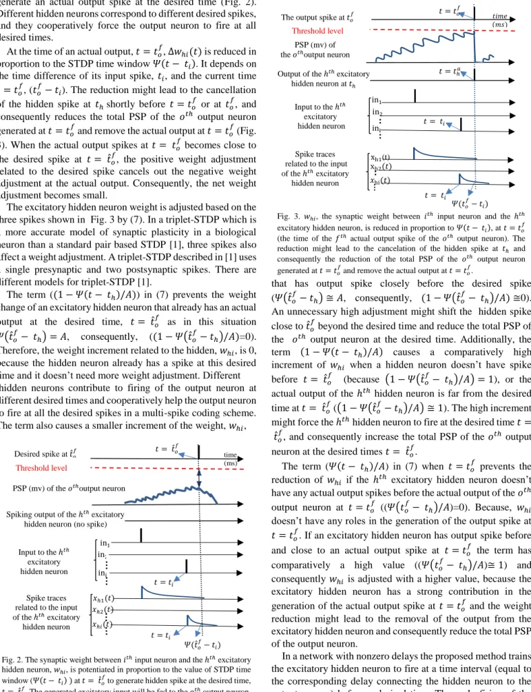
Fig. 2. The synaptic weight between 𝑖𝑡ℎ input neuron and the ℎ𝑡ℎ excitatory
hidden neuron, 𝑤ℎ𝑖, is potentiated in proportion to the value of STDP time
window (𝛹(𝑡 − 𝑡𝑖) ) at 𝑡 = 𝑡̂𝑜 𝑓
to generate hidden spike at the desired time,
𝑡 = 𝑡̂𝑜 𝑓
. The generated excitatory input will be fed to the 𝑜𝑡ℎ output neuron,
and it increases the total PSP of the neuron at the desired time.
Fig. 3. 𝑤ℎ𝑖, the synaptic weight between 𝑖𝑡ℎ input neuron and the ℎ𝑡ℎ
excitatory hidden neuron, is reduced in proportion to 𝛹(𝑡 − 𝑡𝑖), at 𝑡 = 𝑡𝑜 𝑓
(the time of the 𝑓𝑡ℎ actual output spike of the 𝑜𝑡ℎ output neuron). The
reduction might lead to the cancelation of the hidden spike at 𝑡ℎ and
consequently the reduction of the total PSP of the 𝑜𝑡ℎ output neuron
generated at 𝑡 = 𝑡𝑜 𝑓
and remove the actual output at 𝑡 = 𝑡𝑜 𝑓
.
𝑡 = 𝑡̂𝑜 𝑓
Threshold level
PSP (mv) of the 𝑜𝑡ℎoutput neuron
Spiking output of the ℎ𝑡ℎexcitatory
hidden neuron (no spike)
Input to the ℎ𝑡ℎ excitatory hidden neuron 𝛹(𝑡̂𝑜 𝑓 − 𝑡𝑖) in1 in2 ini 𝑡 = 𝑡𝑖 Desired spike at 𝑡̂𝑜 𝑓 𝑡 = 𝑡𝑖 𝑥ℎ1(𝑡) 𝑥ℎ2(𝑡) 𝑥ℎ𝑖(𝑡) Spike traces related to the input of the ℎ𝑡ℎ excitatory hidden neuron time (ms) 𝑡 = 𝑡𝑜 𝑓 Threshold level PSP (mv) of the 𝑜𝑡ℎoutput neuron
Output of the ℎ𝑡ℎexcitatory
hidden neuron at 𝑡ℎ Input to the ℎ𝑡ℎ excitatory hidden neuron 𝛹(𝑡𝑜 𝑓 − 𝑡𝑖) in1 in2 ini 𝑡 = 𝑡𝑖
The output spike at 𝑡𝑜 𝑓 𝑡 = 𝑡ℎ𝑎 𝑡 = 𝑡𝑖 xh1(t) xh2(𝑡) 𝑥hi(𝑡) Spike traces related to the input of the ℎ𝑡ℎ excitatory
hidden neuron
𝑡𝑖𝑚𝑒 (𝑚𝑠)
excitatory hidden neuron increases the total PSP of its successor output neuron at the desired time by the delayed effect of the excitatory hidden spike. However, in the previous situation, where the connections don’t have any delays, an excitatory hidden neuron is trained to fire at the same time as the desired time. Correspondingly, equation (8) is used to adjust 𝑤ℎ𝑖, the synaptic weights between the 𝑖𝑡ℎ input neuron and the ℎ𝑡ℎ excitatory hidden neuron, at time t.
∆𝑤ℎ𝑖(𝑡) = { + ∑[𝑥ℎ𝑖(𝑡 − ɛ𝑜ℎ)(1 − 𝑥𝑜ℎ(𝑡)/𝐴)](𝑤𝑜ℎ/𝐴) 𝑜 , 𝑡 = 𝑡̂𝑜 𝑓 − ∑[𝑥ℎ𝑖(𝑡 − ɛ𝑜ℎ)(𝑥𝑜ℎ(𝑡)/𝐴)] 𝑜 (𝑤𝑜ℎ/𝐴), 𝑡 = 𝑡𝑜 𝑓 0, Otherwise (8)
where 𝑥ℎ𝑖(t) is the spike trace corresponding to the connection between the 𝑖𝑡ℎ input neuron and the ℎ𝑡ℎ excitatory hidden neuron. Each spike in the 𝑖𝑡ℎ input spike train causes a delayed (ɛℎ𝑖) jump in the trace then it decays exponentially by a time constant similar to (3). 𝑥𝑜ℎ(𝑡) is the trace corresponding to the connection between the ℎ𝑡ℎ excitatory hidden neuron and the 𝑜𝑡ℎ output neuron. Each output spike of the ℎ𝑡ℎ excitatory hidden neuron results in a delayed (ɛoh) jump in the trace which decays exponentially by a time constant 𝜏 similar to (3). ɛℎ𝑖 is the delay between the 𝑖𝑡ℎ input neuron and the ℎ𝑡ℎ excitatory hidden neuron, ɛ𝑜ℎ is the delay between the ℎ𝑡ℎ excitatory hidden neuron and the 𝑜𝑡ℎ output neuron. The traces have same amplitude, A, and time constant, 𝜏, as the STDP time window in (2).
The update of 𝑤ℎ𝑖 at 𝑡 = 𝑡̂𝑜 𝑓
in (8) based on the delayed
𝑥ℎ𝑖(𝑡) increases 𝑤ℎ𝑖 by a high value if it has spike shortly before (𝑡̂𝑜
𝑓
− ɛ𝑜ℎ), because in this case 𝑥ℎ𝑖(𝑡̂𝑜 𝑓
− ɛ𝑜ℎ) has a high value. The high increase can lead to generation of an output spike of the ℎ𝑡ℎ excitatory hidden neuron at (𝑡̂
𝑜 𝑓
− ɛ𝑜ℎ). The effect of the generated hidden spike is shifted to the time of the desired spike in the 𝑜𝑡ℎ output neuron after the delay of the connection between the ℎ𝑡ℎ excitatory hidden neuron and the 𝑜𝑡ℎ output neuron, ɛ
𝑜ℎ. This helps the output neuron to generate output spike at the desired time.
The decrement in the second expression of (8) is high if the
𝑖𝑡ℎ input neuron has spike shortly before (𝑡 𝑜 𝑓
− ɛ𝑜ℎ). Consequently, this decrement tries to remove the actual output of the ℎ𝑡ℎ excitatory hidden neuron at (𝑡
𝑜 𝑓
− ɛ𝑜ℎ) and helps the 𝑜𝑡ℎ output neuron to reduce its PSP at the time 𝑡
𝑜 𝑓
(by considering the delay ɛ𝑜ℎ).
2) Weight Learning of theInhibitory Hidden Neurons The connection weight between the ℎ𝑡ℎ inhibitory hidden neuron and the 𝑖𝑡ℎ input neuron, 𝑤̅
ℎ𝑖, is updated similar to (8) by multiplying it with a negative sign as shown in (9).
∆𝑤̅ℎ𝑖(𝑡) = { − ∑[𝑥̅ℎ𝑖(𝑡 − 𝜇𝑜ℎ)(𝑥̅𝑜ℎ(𝑡)/𝐴)]|𝑤𝑜ℎ/𝐴| 𝑜 , 𝑡 = 𝑡̂𝑜 𝑓 + ∑[𝑥̅ℎ𝑖(𝑡 − 𝜇𝑜ℎ)(1 − 𝑥̅𝑜ℎ(𝑡)/𝐴)]|𝑤𝑜ℎ/𝐴| 𝑜 , 𝑡 = 𝑡𝑜 𝑓 0, Otherwise (9)
where 𝜇𝑜ℎ is the delay between the ℎ𝑡ℎ inhibitory hidden neuron and the 𝑜𝑡ℎ output neuron, 𝑥̅
ℎ𝑖(𝑡) is the spike trace corresponding to the connection between the 𝑖𝑡ℎ input neuron and the ℎ𝑡ℎ inhibitory hidden neuron. 𝑥̅
𝑜ℎ(𝑡) is the spike trace related to the connection between the ℎ𝑡ℎ inhibitory hidden neuron and the 𝑜𝑡ℎ output neuron. The delay related the connection between the 𝑖𝑡ℎ input neuron and the ℎ𝑡ℎ inhibitory hidden neuron is 𝜇ℎ𝑖. According to (9) the weight is reduced if the 𝑖𝑡ℎ input neuron has a delayed (𝜇
ℎ𝑖) spike shortly before (𝑡̂𝑜
𝑓
−𝜇𝑜ℎ) to increase the total PSP of the 𝑜𝑡ℎ output neuron at the desired time 𝑡̂𝑜
𝑓
by removing hidden inhibitory spike at or before (𝑡̂𝑜
𝑓
−𝜇𝑜ℎ). Additionally, (9) increases the weight 𝑤̅ℎ𝑖 to generate hidden inhibitory spike at (𝑡𝑜
𝑓
−𝜇𝑜ℎ) to reduce the total PSP of the 𝑜𝑡ℎ output neuron at 𝑡 = 𝑡
𝑜 𝑓
. The reduction of the total PSP removes the actual output spike of the 𝑜𝑡ℎ output neuron at 𝑡𝑜
𝑓 .
It is proposed that hidden neurons receive biofeedback from the readout neurons. Through this biofeedback, the times of desired spikes and actual outputs related to the neurons in the next layer are made available at the hidden layer neurons which use them to adjust their weights appropriately. In this research, we didn’t describe the basis of the biofeedback or model it in detail. The training of the network is stopped when it reaches its goal, i.e. the readout neuron generates actual output spikes at the desired times and all the undesired output spikes of the readout are removed.
D. Classification ability of the proposed method
The weight and delay learning characteristics of the proposed method enable it to train a neuron to fire at desired spike times related to an applied input pattern. In a classification task an input pattern is assigned to the class whose desired spike train is most similar to the actual output of the network. Therefore, the classification ability of the proposed method can be improved if an output neuron is also trained not to fire close to the desired spikes of other classes in addition to firing at the desired times representing to the current class of the input pattern. As a result, the proposed method introduces an additional learning mechanism when a misclassification occurs. The learning algorithm considers two desired spike trains after a misclassification. The first one is related to the class of the applied input spatiotemporal pattern, i.e. the desired spikes of the correct class, and the second one is related to the class that causes the misclassification (incorrect class). Thus, the learning adjusts the readout neurons and hidden neurons learning parameters at the time of each desired spike related to the class that causes the misclassification. It reduces the weights of the readout neuron that have a spike before the desired time. To force the 𝑜𝑡ℎ output neuron to not fire at the 𝑓𝑡ℎ desired spike of class j (𝑡 = 𝑡̂
𝑜 𝑓(𝑗)
) the weights of the
𝑜𝑡ℎoutput neuron are adjusted by the following equation at 𝑡 = 𝑡̂𝑜
𝑓(𝑗) .
The proposed classification learning method adjusts an excitatory hidden neuron weight at the desired spike times (𝑡 = 𝑡̂𝑜
𝑓(𝑗)
) related to the class that causes the misclassification by the following equation similar to (8):
∆𝑤ℎ𝑖(𝑡) = − ∑[𝑥ℎ𝑖(𝑡 − ɛ𝑜ℎ)(𝑥𝑜ℎ(𝑡)/𝐴)] 𝑜
(𝑤𝑜ℎ/𝐴) (11)
An inhibitory hidden neuron weight at 𝑡 = 𝑡̂𝑜 𝑓(𝑗)
is adjusted similar to (9) by the following equation.
∆𝑤̅ℎ𝑖(𝑡) = + ∑[𝑥̅ℎ𝑖(𝑡 − 𝜇𝑜ℎ)(1 − 𝑥̅𝑜ℎ(𝑡)/𝐴)]|𝑤𝑜ℎ/𝐴| 𝑜
(12)
The delay related to an excitatory input of a readout neuron is adjusted by (13) at 𝑡 = 𝑡̂𝑜
𝑓(𝑗)
. Equation (13) is similar to (4).
∆ɛ𝑜ℎ(𝑡) = −∆𝑡𝑜𝑚(𝑡) (𝑥𝑜ℎ(𝑡) 𝑥⁄ 𝑜𝑚(𝑡))
4 (13)
The delay related to an inhibitory input of the readout at 𝑡 = 𝑡̂𝑜𝑓(𝑗) is adjusted through (14) which is similar to equation (6).
∆𝜇𝑜ℎ(𝑡) = +∆𝑡̅𝑜𝑚(𝑡) (𝑥̅𝑜ℎ(𝑡) 𝑥̅⁄ 𝑜𝑚(𝑡))4 (14) The proposed method uses a criterion to control the learning level of every pattern and manage the misclassifications during training and adjust the network learning parameters to increase the inter class separability of the network.
Consider a pattern from class ‘i’ is applied to the network and an actual output of the network is generated. The correlation between the actual output and the corresponding desired spike train of the class ‘i’ is called 𝑐𝑖 which is calculated by the method used in [41] as in (15).
𝑐𝑖= 𝑣𝑑. 𝑣𝑜 |𝑣𝑑||𝑣𝑜|
(15) Where “𝑣𝑑. 𝑣𝑜” denotes the inner product of the two vectors 𝑣𝑑 and 𝑣𝑜. 𝑣𝑑 and 𝑣𝑜 are two vectors with real value components which are generated from spike trains. A desired spike train is convolved with a symmetric Gaussian function to generate 𝑣𝑑. Similarly, 𝑣𝑜 is generated by convolving an actual output spike train with the symmetric Gaussian function. |𝑣| is the length of a vector 𝑣.
A maximum value, 𝑝, and a threshold level, ∆c, for 𝑐𝑖 are considered to control the learning. If the correlation metric, 𝑐𝑖, is less than ∆𝑐 the network learning parameters are updated based on the applied training pattern and its desired spike train without considering any extra criteria. In this situation, the network adjusts its learning parameters to increase its knowledge about the applied training pattern inside the class ‘i’. The low value of the correlation related to the applied training pattern, 𝑐𝑖< ∆𝑐, means that the similarity of the training pattern with the previous trained patterns from the same class ‘i’ is low and the learning parameters of the network should be adjusted
to increase the ability of the network to recognize the patterns inside the class ‘i’.
If 𝑐𝑖 reaches the value of 𝑝, the learning related to the pattern is not applied to the network in the current learning epoch, because the high value of the correlation shows that the knowledge of the presented training pattern is already in the network and it is not necessary to adjust the learning parameters for the current value of 𝑐𝑖. It means that the network has learned the overall distribution of the data from the class ‘i’ and it is not necessary to memorize all the details of the presented training pattern. It also prevents over training of the network.
If 𝑐𝑖 has a value between ∆𝑐 and 𝑝 (i.e. (∆c < ci < p), and 𝑐𝑖 is appropriately higher than the correlation metric related to the other classes to prevent misclassification, then the learning related to the applied pattern is stopped in the current epoch. Therefore, if ∆𝑐 < 𝑐𝑖< 𝑝 and 𝑐𝑖>𝑐𝑗+ ∆𝑐 (where 𝑗 = argmax{𝑘∈{1,2,…,𝑁} & 𝑘≠𝑖}𝑐𝑘, 𝑐𝑘is the correlation metric of the actual output with the 𝑘𝑡ℎ desired spike train, and N is the number of all the classes), the learning adjustment related to the applied pattern from class ‘i’ is not applied to the network in the current epoch. The 𝑐𝑖>𝑐𝑗+ ∆𝑐 denotes that the network can distinguish the class of the applied pattern correctly with an appropriate margin (∆c), therefore it is not necessary to have more training for the current value of 𝑐𝑖 in the learning epoch.
If 𝑐𝑖 has a value between ∆𝑐 and 𝑝, and 𝑐𝑖<cj+ ∆𝑐, it suggests that a misclassification has occurred. In this situation the network learning parameters are updated to enhance the inter class separability of the network by training it to not fire close to the desired spike train of the class that causes this misclassification and to reduce 𝑐𝑗. The learning parameters are also updated to increase the ability of the network to generate the desired spike related to the applied pattern from the class ‘i’ to increase 𝑐𝑖. The reduction of 𝑐𝑗 and the increment of 𝑐𝑖 may change the situation 𝑐𝑖<𝑐𝑗+ ∆𝑐 to 𝑐𝑖>𝑐𝑗+ ∆𝑐 and prevent the misclassification. The training is continued until the maximum number of learning epochs is reached or if the stopping criteria noted in Table I apply.
A 𝑐𝑖 greater than 𝑝 shows that the network is trained to fire appropriately close to the corresponding desired spike train.
TABLE I
THE PROPOSED CLASSIFICATION LEARNING METHOD
when a training pattern from class ‘i’ is presented in a learning epoch: If 𝑐𝑖≤ ∆𝑐,
The corresponding weights and delays are adjusted to increase 𝑐𝑖 i.e.
train the network to generate the 𝑖𝑡ℎ class desired spike.
if ∆𝑐 < 𝑐𝑖< 𝑝 and 𝑐𝑖< 𝑐𝑗+ ∆𝑐
- 𝑐𝑖< 𝑐𝑗+ ∆𝑐 implies that 𝑐𝑖 has a low value and it could cause a
misclassification. So 𝑐𝑖 needs to be increased by learning the 𝑖𝑡ℎ
desired spike train (using (1) for training output neurons’ weights, (4) and (6) for training output neurons’ delays, and (8) and (9) for training hidden Neurons’ weight)
- 𝑐𝑗 needs to be reduced by training the network to not fire close
to the 𝑗𝑡ℎ class desired spike train (using (10) for training output
neurons’ weights, (11) and (12) for training hidden neurons’ weights, (13) and (14) for training Output neurons delays). if (∆𝑐 < 𝑐𝑖< 𝑝 and 𝑐𝑖> 𝑐𝑗+ ∆𝑐) or (𝑐𝑖≥ 𝑝)
The learning parameter adjustment related to the training pattern is not applied to the network in the current epoch. Because 𝑐𝑖 has
reached an acceptable level in this epoch. End
Therefore, similar to the situation where (∆𝑐< 𝑐𝑖≤ 𝑝 and 𝑐𝑖> 𝑐𝑗+ ∆𝑐) the related learning adjustment is not applied to the network. The 𝑝 value is chosen high enough depending on the desired spike trains related to the different classes to guarantee that when 𝑐𝑖> 𝑝, 𝑐𝑖 is appropriately higher than 𝑐𝑗 (𝑐𝑖> 𝑐𝑗+ ∆𝑐). Desired spike trains related to different classes (related to
𝑐𝑖 and 𝑐𝑗) should be chosen in a such a way that the correlation between the desired spike trains are low enough to support the point that if an actual spike train is very similar to the desired spike related to 𝑐𝑖, (𝑐𝑖> 𝑝) then it is appropriately dissimilar to the other classes (𝑐𝑗< 𝑐𝑖− ∆𝑐). The values of 𝑝 and ∆𝑐 are determined by trial and error. In this research the method used in [44] is employed to choose the desired spikes. A sequence of numbers starting from 10ms to 100ms with 10ms time interval is generated. Then a number of firing times are extracted randomly from the sequence to assign each desired spike train corresponding to a class. In this situation, every two spikes have at least 10ms interval. The parameter 𝑝 is set based on the level of precision that the desired spikes should be learnt. In this research when an actual output spike train reaches 90% of accuracy compared to its corresponding desired spike train the learning is stopped, so the learning parameter 𝑝 is set 0.9. The parameter ∆c should be higher than the maximum correlation between the desired spike trains related to different classes. ∆𝑐
is set 0.45 to implement the proposed method.
After training, each testing pattern is applied to the network and the readout actual output spike train is calculated. The correlations between the actual output spike train and the desired spike trains corresponding to all classes are obtained. The input pattern is assigned to the class whose corresponding desired spike train has the maximum correlation value with the actual output spike train.
IV. RESULTS
A. Effect of Network Setups on the Learning Performance First, the effects of the different maximum allowable delays and the number of desired output spikes in each class on the performance of the learning method are explored. Then, the running time for the proposed method is reported. In the following simulation, the performance of the network is first evaluated on the Fisher IRIS data set. The IRIS data features are converted to spike times using population coding as described in [23] where each feature value is encoded by M identically shaped overlapping Gaussian functions where M is set to 40. The IRIS data has four features for each pattern so there are 4×M=160 input spikes obtained which are then applied to 160 input synapses. The high number of input synapses increases the number of input spikes, and consequently reduces the length of silent windows inside a spatiotemporal input pattern and helps the neuron to fire at multiple desired times. Additionally, there are 9 extra input synapses with input spikes at fixed times for all patterns. The fixed times are the same as the times of desired spikes corresponding to all classes. These inputs act as bias inputs [21] and act as the reference start times in a multi-spike coding scheme. There are 360 hidden neurons in the hidden layer. The total time duration of the input
spatiotemporal pattern is set to 100ms, T=100ms. 1) The effect of maximum allowable delays
Similar to [24], 50% of the IRIS data were selected randomly and used as training data and the remaining used for testing. The accuracy of the proposed method on the testing data reaches its highest value, 95.1%, when the maximum allowable delay, D, is 3ms and there is a single readout neuron.
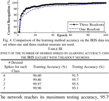
In Table II, the accuracies of the proposed method for different delays when there are three readout neurons (each corresponding to a class) in the network are shown. The accuracy of the method on the testing data reaches its maximum value when D=3ms (Table II). The accuracy of the proposed method on the testing data is increased from 95.1% to 95.7% when the number of readout neurons is increased from one to three when D=3ms. In Fig. 4 the accuracy of the learning algorithm on the training data is shown when a single readout neuron and three readout neurons are used. All these procedures are repeated independently for 40 different runs and the mean value of the 40 results are reported. Different random, initial weights and different random selection of the training and testing data are used for the different runs. When the number of readout neurons is increased the number of learning parameters is also increased. Therefore, the readout neurons learn a lower number of training patterns compared to the situation where a single readout neuron is used, where the readout neuron should learn patterns related to all classes. Subsequently, they can learn the input patterns better compared to the situation that a single readout neuron is used. For higher values of maximum allowable delays the cooperation between weight adjustment and delay adjustment is reduced and it leads to a lower accuracy. A higher delay adjustment causes a higher shift in the delayed effect of input spikes and this higher shift might destroy previous weight training that was based on the previous value of the delay.
Synaptic delays at chemical synapses usually take values from 1ms to 5ms. The minimum value of a synaptic delay is 0.3ms. Synaptic delay also can take a value higher than 5ms [45]. Different researchers use different maximum values for range [1, 16]ms. The results in this section show that for this configuration, 3ms is an optimal value for the maximum synaptic delay. In the following simulations Max-Delays are set to 3ms.
2) The effect of the number of desired spikes
In the following experiment, the accuracy of the proposed method is obtained for different numbers of desired spikes corresponding to each class (TableIII).
TABLE II
THE EFFECT OF THE DIFFERENT MAXIMUM ALLOWABLE DELAYS ON IRIS
DATA RECOGNITION.50% OF THE DATA ARE USED AS TRAINING DATA. Max-Delays (ms) Training Accuracy (%) Testing Accuracy (%)
1 99.8 95.3 3 99.8 95.7 4 99.6 95.7 5 99.6 95.3 7 99.6 94.6 10 98.9 94.5
The network reaches its maximum testing accuracy, 95.7%, when three desired spikes are used in each desired spike train. A very high number of desired spikes in each desired spike train (i.e. for a desired spike train with 100ms duration and 10ms minimum inter spike interval the highest number of desired spikes is 10) reduces the performance of the learning method as this increases the complexity of the learning task and the network should be trained to fire at a higher number of desired instances with a limited number of learning parameters. For instance, the testing accuracy of the proposed method is reduced from 95.7% to 81.0% when the number of desired spikes is increased from 3 to 7 (Fig. 5).
The time distances between desired spikes of different classes are reduced when there is a high increase in the numbers of desired spikes. Therefore, a small deviation in the times of output spikes can cause a switching from one class to the other one and reduces the accuracy. On the other hand, a lower number of desired spikes reduces the complexity of the learning task therefore the training accuracy will be increased. However, a very low number of desired spikes lead to a low testing accuracy. For example, when the number of desired spikes is reduced from three to one the testing accuracy is reduced from 95.7% to 95.1%. It shows that a single spike cannot capture enough information from training data and consequently it reduces the testing accuracy despite of a comparably high training accuracy of 99.9%. Moreover, the distributions of spikes in the spatiotemporal input patterns compared to desired spikes also affect the accuracy and the relation between the number of desired spikes and the accuracy is not a simple linear function (Fig. 5).
3) Evaluation of the running time
MATLAB simulations were carried out on a quad core PC with 3GHz and 16GB of RAM. The running times required for
each learning epoch of the proposed method are reported in Table IV. The running time related to a learning epoch is measured ten times and the mean value is reported for each number of input synapses. The running time is increased by increasing the maximum allowable delays, D. For instance the method needs 5.2 seconds to execute a learning epoch when D = 1ms. However, the running time is increased to 15.9 seconds when D is increased to 7ms. Because, at each time step the learning algorithm should check the events at the previous time steps depending on the delays. A higher number of previous time steps should be considered for a higher value of delays. Therefore, the computational complexity of the method and consequently the running time is increased when the delay is increased.
The running times of a learning epoch of the proposed method are measured for different numbers of training patterns. The number of training patterns is increased from 15 to 135. IRIS data set is used to train the algorithm. Fig. 6 (a) shows the relationship between the running times and the number of training patterns. The fitted line shown in Fig. 6 (a) is obtained by fitting the data points to a one-dimensional polynomial. The line is described by the equation 𝑇(𝑛) = 0.1128𝑛 + 1.593. The time complexity of the process related to the equation is linear, i.e. it is O(n) using the big O notation. It shows that the running time increases linearly with the number of training samples.
Random spatiotemporal input patterns with different numbers of inputs are used to analyse the complexity of the learning algorithm as a function of the number of input synapses. There are three classes similar to IRIS data in the randomly generated data. A spike train composed of three spikes are considered as desired spike train for each class like the desired spike used for IRIS data. The spike times in each input spatiotemporal pattern are generated by a uniform
Fig. 4. Comparison of the learning method accuracy on the IRIS data training set when one and three readout neurons are used.
0 20 40 60 80 100 90 92 94 96 98 100 Epoch C o rr ec t R ec og n it io n ( %) Three Readouts One Readout TABLE III
EFFECT OF THE NUMBER OF DESIRED SPIKES ON LEARNING ACCURACY USING THE IRIS DATASET WITH 3 READOUT NEURONS
# Desired Spikes for each
Class
Training Accuracy (%) Testing Accuracy (%)
4 96.60 91.5
3 99.80 95.7
2 99.97 95.5
1 99.90 95.1
Fig. 5. Recognition accuracy for different numbers of desired spikes.
1 2 3 4 5 6 7 8 80
85 90 95
Number of desired spikes
A c cu r a c y ( % ) TABLE IV
EFFECT OF THE MAXIMUM ALLOWABLE DELAY (D) ON THE RUNNING TIME OF THE PROPOSED METHOD USING THE IRIS DATASET
Max-Delays (ms) Running Time (sec) Max-Delays (ms) Running Time (sec) 1 5.2 5 12.4 3 9.2 7 15.9 (a) (b)
Fig. 6. The runing time of a learning epoch is increased linearly as a function of (a) the number of training patterns, and (b) the number of input synapses.
0 20 40 60 80 100 120 140
0 10 20
Number of Training Patterns
T im e ( s) 0 200 400 600 800 1000 5 10 15
Number of Input Synapses
T
im
e
(s
distribution. The values of spike times are extracted randomly from (0, 100) interval. The number of input synapses is changed from 100 to 1000, and an input spike is considered for each input synapse. Then, the running time for each learning epoch is calculated to analyse the complexity of the learning method. In this experiment there is a fixed number of 75 training patterns. Fig. 6 (b) shows the evolution of the running time in terms of the number of input synapses. Additionally, a line fitted with the obtained data points is plotted. The dependency between running time and the number of inputs indicates a linear time complexity, i.e. O(n).
B. Comparison with State-of-the-art Methods
In the following simulation, first the proposed method is compared with the method proposed by Sporea et. al. [28]. In this case 75% of the total IRIS data for each class is considered as a training set and the remaining 25% is used for testing as in [28]. The results are shown in Table V. The accuracy of the proposed method on the training is 99% which is higher than the method proposed in [28], 96%. The proposed method also achieved a higher testing accuracy of96% (compared to 94% achieved by [28]).
Similar to the biologically plausible structure used in [18], each of the 169 input neurons is connected randomly to a limited number of neurons (40 neurons) in the hidden layer which consists of a population of 360 neurons. There are no sub-connections and every two neurons in two subsequent layers are connected by a single connection similar to the biologically plausible neural network in Izhikevich’s work[18]. The proposed learning algorithm is designed to manage the training of a large number of SNs by local events such as spike trace which takes place at the location of each synapsis. There are three output neurons in the output layer and all the hidden neurons are connected to the three output neurons. The network proposed in [28] uses the timing of a single spike of an input neuron for each feature. The four input neurons are fully connected to 10 neurons in the hidden layer. Every two neurons in two subsequent layers are connected by 12 sub-connections with different delays from 1 to 12ms. All the neurons in the hidden layer are fully connected to an output neuron. The performance of the method in [28] on the IRIS data is shown in Table V.
In order to compare the accuracy of the proposed method with that achieved by other existing methods, 50% of the data samples from the IRIS dataset are selected randomly to construct training data and the remaining 50% used for testing. The testing results are summarised in Table VI. The accuracy of the proposed method on the training and testing data are 99.7% and 95.7%, respectively. The testing accuracy of the
proposed method, 95.7%, is comparable with the best result achieved for the state of the art methods on IRIS data set. The proposed method has a high training accuracy, 99.7%.
The proposed method converges for all trials because it doesn’t have the silent neuron problem. It has remote supervised spikes. Additionally, it solves the problem of silent windows in a spatiotemporal input pattern by delay learning. A silent window can prevent generation of desired spikes and consequently it can cause learning convergence problem. These characteristics of the proposed method make it appropriate for learning multiple spikes. The accuracies of the proposed method are calculated for all trials, and there are not any rejected results. In contrast the convergence rate of SpikeProp is investigated in [24] and as it has a problem with silent neurons it cannot converge for all trials and as a result those trials with low accuracies are removed from the reported results [24].
The Breast Cancer Wisconsin (Diagnostic) data set (WBCD) from the UCI machine learning repository is used as the second dataset to evaluate the proposed method and to compare it with the other state of the art methods as shown in Table VII. WBCD contains 699 samples. The samples belong to two different classes (malignant and benign categories) where 458 samples are from the first category and 241 samples are from the second category. A total of 120 samples are selected randomly from each category to construct the training set and the remaining data is used for testing. The proposed method has an accuracy comparable with the best accuracy achieved by the other state of the art methods (Table VII).
One advantage of SNNs is that they use spikes to communicate between neurons. However, in the classical neural networks real values are used to transfer data between neurons. Each spike can be encoded by a binary bit however a real value needs a high number of bits to be transferred between neurons depending on the precision that is required for the values. As shown in Table VI and Table VII, the proposed method using spikes for communication between neurons and can achieve better or comparable accuracies with the state-of-the-art rate–based models including Deep Belief Network (DBN) and Autoencoders.
TABLE V
COMPARISON WITH THE MULTILAYER SNN PROPOSED IN [28] ON THE IRIS
DATASET
Method Training Accuracy (%) Testing Accuracy (%) Sporea et. al.[28] 96 94
The proposed method 99.3 95.8
TABLE VI
COMPARISON WITH OTHER METHODS ON THE IRIS DATASET
Method Testing Accuracy (%) Spiking Methods RBF [50] 92.6 SWAT [51] 95.3 SpikeProp [24] 95 QuickProp [23] 92.3 RProp [23] 93.2 RBF [53] 89 SNN (Bako) [52] 83.4 Proposed Method 95.7 Non-Spiking Methods K-Means [50] 88.6 SOM [50] 85.33 Matlab BP [51] 95.5 Matlab LM [51] 95.7 TEST [55] 91.7