Temporal Optimization Planning for Fleet Repositioning
Kevin Tierney
and
Rune Møller Jensen
IT University of CopenhagenRued Langgaards Vej 7, DK-2300, Copenhagen S, Denmark
{kevt,rmj}@itu.dk
Abstract
Fleet repositioning problems pose a high financial bur-den on shipping firms, but have received little atten-tion in the literature, despite their high importance to the shipping industry. Fleet repositioning problems are characterized by chains of interacting activities, but state-of-the-art planning and scheduling techniques do not offer cost models that are rich enough to repre-sent esrepre-sential objectives of these problems. To this end, we introduce a novel framework called Temporal Optimization Planning (TOP). TOP uses partial or-der planning to build optimization models associated with the different possible activity scenarios and ap-plies branch-and-bound with tight lower bounds to find optimal solutions efficiently. We show how key aspects of fleet repositioning can be modeled using TOP and demonstrate experimentally that our approach scales to the size of problems considered by our industrial collaborators.
Introduction
Liner shipping networks transport containerized cargo through regularly scheduled shipping routes. Fleet repositioning problems consist of moving ships between services in a liner shipping network in order to better orient the overall network to the world economy and to ensure the proper maintenance of ships. Thus, fleet repositioning involves sailing and loading activities sub-ject to complex handling and timing restrictions. As is the case for many industrial problems, the objective is cost minimization (including costs for CO2 emissions and pollution), and it is important that all cost ele-ments, including the ones that are only loosely coupled with activity choices, can be accurately modeled.
Optimization problems that involve chains of activ-ities with complex interactions, like fleet repositioning problems, are hard to represent as mathematical pro-grams. AI-planning and OR-scheduling offer a wide range of approaches to allocate interacting activities over time, but it has been observed in both fields (e.g., (Karger, Stein, and Wein 1997; Smith, Frank, and J´onsson 2000)) that the compound objectives of real-world problems often are hard to express in terms of the simple objective criteria like makespan and tardi-ness minimization considered in these approaches.
In this paper, we introduce a novel general frame-work called Temporal Optimization Planning (TOP) and show that it can model key aspects of fleet repo-sitioning problems. The core idea of TOP is to asso-ciate durative planning actions with optimization model components and use planning algorithms to build and search through complete optimization models that are associated with the different activity scenarios of the problem. In contrast to advanced temporal planning languages (Fox and Long 2006), TOP does not enforce a strong semantic relation between planning actions and optimization components. The format of optimization components can be chosen freely by the model designer as long as the set of complete plans corresponds to the set of activity scenarios of the problem.
In this way, TOP allows general optimization models to be constructed, but at the same time makes it pos-sible to naturally represent and explore complex inter-actions between durative activities with the expressive action models of AI-planning and its powerful search algorithms. In fact, TOP accommodates any optimiza-tion model over real-valued variables and thus is a sim-ple way to reason about interacting durative activities in such models.
We solve TOP problems by an optimization version of partial-order planning (Penberthy and Weld 1992) based on a branch-and-bound and demonstrate the ap-proach for linear optimization models. We define a gen-eral lower bound for partial plans in the naturally oc-curring case where the minimum costs of optimization components are non-negative. We show that this bound can be improved by an extension of thehmaxheuristic
(Haslum and Geffner 2000) that makes it possible to estimate the cost of required actions not currently in the plan.
The TOP framework is validated experimentally on a set of fleet repositioning problems developed in col-laboration with a liner shipping company. We provide a basic model of a fleet repositioning problem that gives a first step towards solving such problems in TOP. We include key aspects such as the temporal interaction be-tween ships and complex cost objectives such as sailing fuel consumption and the fixed cost of ships over time. Our experimental evaluation shows that the TOP
ap-proach scales to the size of problems faced by the in-dustry and that our lower bounds are tight enough to reduce the total computation time by orders of magni-tude.
The remainder of the paper is organized as follows. First we describe fleet repositioning problems, followed by a formalization of TOP along with a description of thehcostmax heuristic for estimating lower bounds of par-tial plans. Then we describe our model of a simple fleet repositioning problem and we present experimental re-sults showing the performance of the TOP framework with several plan selection heuristics. Finally, we draw conclusions and discuss directions for future work.
Fleet Repositioning
Liner shipping networks consist of multiple services, which are circular routes that connect a sequence of ports. Each service consists of one or more ships that maintain a weekly schedule. That is, each port on a ser-vice is visited by a ship on the same day each week, and a service is assigned as many ships as are necessary to maintain weekly frequency. Ships are periodically repo-sitioned, in which they are moved from their current service to some other service. Shipping firms reposition their ships so that they can undergo regular mainte-nance, be returned to their owner, or to better match ships to markets.
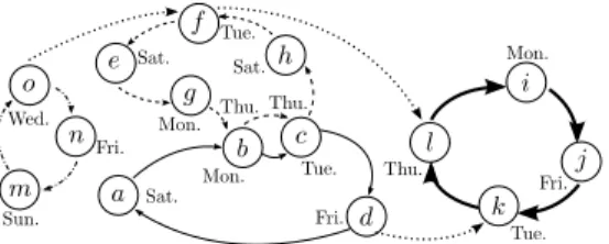
Consider the example repositioning problem shown in Figure 1 in which a new service is being started and requires ships to sail on it. This example involves the temporal alignment of several ships. First a ship from the service on the left must sail to the dashed line ser-vice, but the ship on the dashed line service may not leave for its goal service until its replacement ship has arrived, and cargo has been transshipped. Second, the two ships sailing to the service on the right must have a time spacing of exactly one week. Complicating mat-ters further is that shipping firms want to reposition their ships as cheaply as possible.
Fleet repositioning problems can be even more com-plicated than the example given, with several ships re-placing one another in long chains. Aligning the ships temporally and finding a minimum cost plan of activ-ities presents a significant challenge. The possible ac-tivities that a ship may undertake during repositioning is given as follows.
• Ships can leave or enter a service only at a port on days when the port is scheduled to be called.
• Ships must sail between their minimum and maxi-mum speed, the cost of which is a function of the ship’s speed and draft,
• Ships can idle at a port, incurring a fixed cost per hour (in shipping parlance,hotel cost).
• Cargo can be on/off loaded, resulting in a fee per container moved.
• Cargo can be directly transhipped between ships, in-curring a reduced per container fee.
Figure 1: An example fleet repositioning problem in-volving three ships. Two ships are being repositioned from their initial services (solid, dashed) to a new ser-vice (bold solid). The ship on the dashed serser-vice is be-ing replaced by a ship from the dashed-dotted service, which will cease operations. Circles represent ports and are labeled with the day the service calls the port.
• Ships can move equipment (empty containers) to where it is needed, reducing the overall cost of repo-sitioning.
• Ships may satisfy certain demands in the shipping network for a profit.
A number of constraints pose restrictions on when the given activities may take place. Ships must be replaced by another ship in order to leave their service, except for certain, designated ships. Ships may not load or un-load cargo in certain ports due to cabotage restrictions, which are laws that prevent foreign ships from offer-ing domestic services. If multiple ships are enteroffer-ing the same service, they must enter one week apart in dis-tance or time from one another. In addition, multiple ships must alternate in size such that if there are sev-eral ships entering a service, no two ships of the same capacity should follow one another.
Given the high expense of repositioning, the goal of fleet repositioning problems is to find a scenario of ac-tivities, which involve continuous decisions regarding sailing time and cost configurations, associated with a lowest cost optimization model.
The fleet repositioning problem is difficult to solve for existing scheduling and planning methods.
Scheduling is concerned with the optimal allocation of scarce resources to activities over time (Karger, Stein, and Wein 1997), and scheduling research has focused on problems that only involve a small, fixed set of choices, while planning problems like fleet repositioning often in-volve cascading sets of choices that interact in complex ways (Smith, Frank, and J´onsson 2000). Another lim-itation is that mainstream scheduling research has fo-cused predominately on optimization of selected, simple objective criteria such as minimizing makespan or min-imizing tardiness (Smith 2005). More general objective criteria are required in order to solve fleet repositioning problems.
Integer Programming (IP) has successfully been ap-plied to solve classical planning problems using com-petitive encodings based on the planning graph heuris-tic (Van Den Briel, Vossen, and Kambhampati 2005). An earlier version of this approach has also been used
to extend classical planning with possibly continuous state variables over which linear constraints and objec-tives can be stated (Kautz and Walser 1999). A limi-tation of these encodings is, though, that they are un-able represent continuous time. In general, it is difficult to represent partial-order planning with IP since the number of actions in a partial-order plan in principle is unbounded. A SAT encoding of actions with contin-uous duration (Shin and Davis 2005), however, shows that other encodings of continuous time using IP may be possible, but this encoding currently does not cover any objective criteria except minimizing the number of unique time points in the plan.
Within AI, there exists domain independent planners for temporal planning languages and specialized appli-cation planners.With respect to the former, while early approaches had limited scalability (e.g., (Ghallab and Laruelle 1994; Penberthy and Weld 1995)), a number of powerful solvers have recently been developed for planning languages with durative actions, real-valued state variables, and linear change of quantities dur-ing action execution (e.g. (Coles et al. 2009; 2010; Li and Williams 2008; Shin and Davis 2005)). These planning languages can model domains where activi-ties depend on shared resources like electric power dur-ing execution, which is a typical situation for popular application domains within robotics and aerospace sys-tems (e.g., (Frank, Gross, and Kurklu 2004; Muscettola 1993)). However, the fleet repositioning problem in-volves decoupled actions that intersect only temporally. Furthermore, most of these domain independent and application specific planning systems only allow simple objective criteria like makespan minimization. A no-table exception is Sapa (Do and Kambhampati 2003), which can represent multi-criteria objectives covering any combination of makespan minimization and min-imization of fixed action and resource costs. On the other hand, Sapa only handles discrete time and fixed action durations.
Recently, the 2008 International Planning Compeiti-tion (Helmert, Do, and Refanidis 2008) featured a net benefit optimization category with several entries:
hsp∗, MIPS-XXL, and Gamer. These planners are
un-able to reason temporally, and only support fixed action costs in their objective, preventing them from handling many aspects of fleet repositioning problems, such as hotel costs and variable action cost. Linear Program-ming has been used to strengthen plan length estima-tion (e.g. (Bylander 1997; Van Den Briel et al. 2007)), however these approaches do not handle a cost-based objective or temporal setting, with the ordering relax-ation in (Van Den Briel et al. 2007) being particularly troubling for a temporal planner.
Temporal Optimization Planning
In the absence of a suitable method for solving fleet repositioning problems, we introduce Temporal Opti-mization Planning (TOP). TOP diverges fundamen-tally from classical AI-planning approaches byintro-ducing two sets of variables that decouple the planning problem from the optimization model. Thus, the opti-mization model is not tightly bound to the semantics of actions. Actions are merely used as handles to op-timization components that are built together to com-plete optimization models using partial-order planning. This decoupling makes it possible to formulate any ob-jective that can be expressed by the applied optimiza-tion model. Moreover, computaoptimiza-tionally expensive ac-tion models including real-valued state variables and general objective functions are avoided.
In contrast to the current trend in advanced temporal planning languages, TOP bypasses computationally ex-pensive dense time models of shared resources like elec-tric power consumption during activities. These models are important for the robotic or aerospace applications that often are targeted in AI-planning (e.g., (Frank, Gross, and Kurklu 2004; Muscettola 1993)), but TOP focuses on more physically separated activities where resources are exclusively controlled.
On the other hand, while this decoupling offers some new possibilities, it makes TOP less capable of solving traditional planning problems where a strong coupling is assumed as well as problems that fit within a classical scheduling model.
TOP is built off a state variable representation of propositional STRIPS planning (Fikes and Nilsson 1971). TOP utilizes partial-order planning (Penberthy and Weld 1992), and extends it in several ways. First, an optimization model is associated with each action in the planning domain. This allows for complex ob-jectives and cost interactions that are common in real world optimization problems to be easily modeled. Sec-ond, instead of focusing on simply achieving feasibility, TOP minimizes a cost function. Finally, begin and end times can be associated with actions, making them du-rative. Such actions can have variable durations that are coupled with a cost function.
Formally, let V ={v1,· · ·, vn} denote a set of state
variableswith finite domainsD(v1),· · ·, D(vn). Astate
variable assignment ωis a mapping of state variables to values {vi(1) 7→ di(1),· · ·, vi(k) 7→ di(k)} where di(1) ∈ D(vi(1)),· · ·, di(k) ∈ D(vi(k)). We also define vars(ω) as the set of state variables used inω.
A TOP problem is represented by a tuple P =hV,D,A,I,G, pre,eff,x, obj, coni,
where D is the Cartesian product of the domains D(v1)× · · · ×D(vn), A is the set of actions, I is a
total state variable assignment (i.e. vars(I) =V) rep-resenting the initial state,Gis a partial assignment (i.e. vars(G)⊆ V) representing the goal states,preais a
par-tial assignment representing the precondition of action a, effa is a partial assignment representing the effect
of action a1, x∈
Rm is a vector of optimization vari-1
In practice, is it often more convenient to represent ac-tions in a more expressive form, e.g. by letting the precon-dition be a general expression on states prea :S →B and
ables2 that includes the begin and end time of each action, xa
b and xae respectively, for all actions a ∈ A,
obja : Rm→ Ris a cost term introduced by action a,
and cona : Rm → B is a constraint expression
intro-duced by action a with cona |= xab ≤ x a
e ∧ xab ≥ 0 ∧
xae≥0.
Let S ={ω|vars(ω) = V} denote the set of all the possible states. An action a is applicable in s ∈ S if prea ⊆ s and is assumed to cause an instantaneous
transition to a successor state defined by the total as-signment
succa,s(v) =
eff
a(v) ifv∈vars(effa),
s(v) otherwise.
We further defineMa=min{obja|cona}, which is the
optimization model component introduced by actiona. A temporal optimization plan is represented by a tu-ple hA, C, O, Mi, where A is the set of actions in the plan, C is a set of causal links, O is a set of ordering constraints of the forma≺b, wherea, b∈A, andM is an optimization model associated with the plan. M is defined by min X a∈A obja(x) s.t. xai e ≤x aj b ∀ai ≺aj ∈O (1) cona(x) ∀a∈A (2)
The objective of M is to minimize the sum of the costs introduced by actions. The first constraint ensures that the start and end time of actions are consistent with the plan, and second constraint requires that each action constraint is satisfied. Let cost(π) denote the cost of an optimal solution toM to a partial planπ.
Anopen condition −→µ bis an unfulfilled precondition µ of actionb ∈A, that is, µ ∈preb and ∀a∈A, a
µ
−→
b 6∈ C. An unsafe link is a causal link a −→µ b that is threatened by an action c such thati) vars(µ)∈effc,
ii)µ6∈effc, and iii){a≺c≺b} ∪O is consistent.
To deal with durative actions in TOP we need to keep track of another type of flaw called inter-ference. We adopt an interference model based on the exclusive right to state variables (Sandewall and R¨onnquist 1986). Thus, two actionsaandbinterfere if vars(effa)∩vars(effb)6=∅andOimplies neithera≺b
norb≺a.
An open condition flaw −→µ b can be repaired by linking µ to an action a such that µ ∈ effa and by
posting an ordering constraint over a and b. Thus,
represent conditional effects like resource consumption by letting the effect be a general transition function, depending on the current state ofS,effa,s:S →S. Such expressive
implicit action representations may also be a computational advantage. We have chosen a ground explicit representa-tion of acrepresenta-tions because it simplifies the presentarepresenta-tion and more expressive forms can be translated into it.
2
In a slight abuse of notation, we sometimes letxdenote a set rather than a vector.
Algorithm 1Optimization planning algorithm, based on (Williamson and Hanks 1996).
1: functionTOP(I,G)
2: Π← {InitialTOP(I,G)}
3: πbest←null
4: u← ∞.Cost of the incumbent (upper bound)
5: whileΠ6=∅do
6: π←SelectPlan(Π)
7: Π←Π\ {π}
8: if NumFlaws(π) = 0∧Cost(π)< uthen
9: u←cost(π)
10: πbest←π
11: else if EstimateCost(π)< uthen
12: f ←SelectFlaw(π)
13: Π←Π ∪RepairFlaw(π, f)
14: returnπbest
C←C∪{a−→µ b}andO←O∪{a≺b}. In the case that a6∈A,A←A∪ {a} andO←O∪ {a0≺a, a≺a∞}.
An unsafe linka−→µ b that is threatened by action c can be repaired by either adding the ordering constraint c ≺a (demotion) or b ≺c (promotion) toO. Similar to unsafe links, an interference between actionsaandb can be fixed by posting eithera≺bor b≺atoO.
Together, open conditions, unsafe links and inter-ferences constitute flaws in a plan. Let f laws(π) = open(π)∪unsafe(π)∪interfere(π) be the set of flaws in the planπ, whereopen(π) is the set of open conditions, unsafe(π) is the set of unsafe links, andinterfere(π) is the set of interferences. We say that π is a complete plan if|f laws(π)|= 0, otherwiseπis apartial plan. A plan π∗ is optimal if it is feasible and for all feasible solutions π,cost(π∗)≤cost(π).
Linear Temporal Optimization Planning
To solve fleet repositioning problems, we introduce lin-ear temporal optimization planning (LTOP). In LTOP, all of the optimization models associated with planning actions have a linear cost function and a conjunction of linear constraints. Thus,objais of the formcax0, whereca∈Rm andcona is of the formV1≤i≤na(α a
ix0 ≤βi),
where αa
i ∈Rm, βi ∈R andna is the number of
con-straints associated with actiona. Thus,Ma andM are
linear programs (LPs).
Algorithm 1 shows a branch-and-bound algorithm that finds an optimal plan to an LTOP problem. First, an initial planπinitis created by theInitialTOP
func-tion (line 2). We define πinit = h{a0, a∞},∅,{a0 ≺
a∞}, Minit}i, wherea0is an action representingI with
prea0 =∅ andeffa0 =I, a∞ is an action representing
Gwithprea∞ =Gandeffa∞ =∅, andMinit is an
opti-mization model with no objective and two constraints, cona0 and cona∞, which are special constraints on the
dummy actions a0 and a∞ such that cona0 = (x
a0 b = xa0 e ∧x a0 b ≥0) andcona∞ = (x a∞ b =x a∞ e ∧x a∞ b ≥0).
The optimization variables xa0
b , x a0 e , x a∞ b and x a∞ e
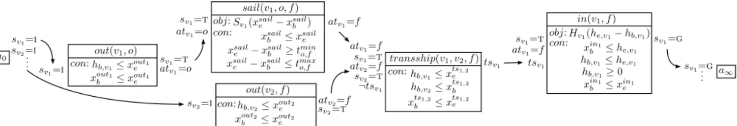
Figure 2: A partial temporal optimization plan from Figure 1 showing the ship sailing from the dash-dotted service to the dashed service (v1) and the ship sailing from the dashed service to the bold, solid service. Boxes represent actions and contain associated optimization models. Arrows between boxes show causal links. The optimization variablesxa
b andx
a
e represent the begin and end time of actiona, andhb,v,he,v are the begin and end hotel time of
vesselv respectively. Each vesselv is associated with a state variable sv with a domain of {i,t,g} which indicate
thatv is on its initial service, in transit or at its goal service, respectively.
respectively.
The algorithm then selects a plan from Π (line 6) and checks to see if it is a complete plan. If the plan is complete, its cost is compared with the current upper bound (u), and if the cost is lower, theincumbent πbest
is replaced with the current planπand the upper bound is updated (lines 9 and 10). Whenπis a partial plan, an estimated lower bound of the plan is compared with the cost of the incumbent solution (line 11). If the esti-mated cost of the plan is higher, the plan is discarded. Otherwise, a flaw is selected and repaired (lines 12 and 13). This process is repeated until Π is empty, at which point the current incumbent is returned, if there is one. Algorithm 1 is guaranteed to find the optimal solu-tion (if there is one) as long asEstimateCostdoes not overestimate the cost of completing a partial plan. To prune as much of the branch-and-bound tree as possi-ble, we need tight lower bounds. If we require that the cost of each action subject to its constraints is non-negative, we can prove that cost(π) is such a lower bound.
Proposition 1. Given any valid partial plan π =
hA, C, O, MiwhereMa≥ 0 ∀a∈A,cost(π)≤cost(¯π)
for any completion π¯ of π.
Proof. Letπ0beπwith a single flaw repaired. The flaw is either i) an unsafe link, ii) an interference, iii) an open condition being satisfied by an action in the plan, oriv) an open condition being satisfied by an action not in the plan.
In cases i and ii the flaw is repaired by adding an ordering constraint to π, which further constrains π, thus cost(π) ≤ cost(π0). Case iii results in a new causal link and an ordering constraint, and is there-fore the same as cases i and ii. In case iv, the ac-tion’s optimization model is added to π, but since the cost function of the action must be non-negative under its constraints, cost(π0) cannot be less than cost(π). By applying this argument inductively on the com-plete branch-and-bound subtree grown fromπ, we get cost(π)≤cost(¯π) for any completion ¯πofπ.
Heuristic Cost Estimation
Althoughcost(π) provides a reasonable lower bound for π, the bound is only computed over actions in the plan. It can be strengthened by also reasoning over actions that are not in the plan. We present an extension of the hmaxheuristic (Haslum and Geffner 2000),hcostmax, which
estimates the cost of achieving the open conditions of a planπ. Let hcostmax(ω, π) = 0 ifω⊆effsπ, else f(ω, π) ifω={µ}, else g(ω, π) if|ω|>1,
f(ω, π) = min{a∈A\A|µ∈effa}{Ma+hcostmax(prea, π)},
g(ω, π) = maxµ∈ω{hcostmax({µ}, π)},
where ω is a partial state variable assignment, µ is a single state variable assignment v 7→ d, and effsπ =
S
a∈Aeffa. The heuristic takes the max over the
esti-mated cost of achieving the elements in the given as-signment ω. The cost is zero if the elements are al-ready in π, otherwise the minimum cost of achieving each element is computed by finding the cheapest way of bringing that element into the plan.
Proposition 2. Given any valid partial plan π =
hA, C, O, Mi where Ma ≥ 0 ∀a ∈ A, cost(π) +
hcostmax(open(π), π)≤cost(¯π)for any completion π¯ of π.
Proof. We have hcost
max(ω, π) =
P
a∈RMa, where R is
a set of actions not currently in π (R∩A = ∅) that are required to resolve ω and among such sets has the minimum cost. Thus, any completion ¯π of π as de-scribed in Proposition 1 must at least increasecost(π) byhcost
max(ω, π) =
P
a∈RMa.
Modeling Fleet Repositioning
We describe an LTOP model of fleet repositioning prob-lems that represents a first step towards modelling and solving fleet repositioning problems. Our model repre-sents a subset of fleet repositioning that captures its dif-ficult elements, while excluding excessive detail. We fo-cus on several key components of the fleet repositioningproblems that form the basis for more difficult versions includingi) the temporal interaction between ships in a sequence of replacements,ii) variable ship sailing dura-tions,iii) sailing costs that vary linearly with the sailing duration, andiv) ship hotel costs that must span mul-tiple actions.
Given a set of services, the goal is to carry out a se-quence of repositionings in which a ship on each service is moved to the next service in the sequence at minimal cost. A ship may not be moved from its service until replaced by another ship, except in the case of the first service in the sequence.
Ships cease operations on their initial service through the action out and begin operations on a service through thein action. During the time in betweenout andin, ships are charged their hotel cost, which is rep-resented in the objective of the in action. The hotel cost objective is given in theout action for ships that do not have a target service, and will therefore not use theinaction, such as a ship being returned to its owner or heading for repairs.
Ships mustsail between ports within their minimum and maximum speed, incurring a cost that varies lin-early with the speed. In order for a ship to replace another ship on a service, they must transship their cargo. Transshipments in our model are instantaneous, free actions that require both ships to simultaneously be at a port where it is lawful for the ships to perform a transshipment. Transshipments are only allowed at ports in which a ship is lawfully able to transfer cargo, which we are able to represent by simply not including transshipment actions between ships at ports where it would be unlawful.
Implicit in our model are wait actions. Such an action does not need to be explicitly given, because actions, even those that are ordered or linked, are not required to start directly after one another. The objective of this implicit action is given by the hotel cost computed in theout andin actions.
Figure 2 shows a fleet repositioning partial plan in the LTOP framework in which two ships are moved off of their initial services (outaction), and meet at portf where they transship cargo (transship action). Shipv1 then begins service at port f (in action), freeingv2 to continue to a different service or undergo maintenance. Notice how the objective for the hotel cost for v1, rep-resented byhb,v1 andhe,v1, is computed in thein(v1, f)
action, but the bounds for the hotel cost are updated throughout the partial plan. This allows the LP to com-pute a more accurate bound throughout the planning process. Multiple actions are therefore contributing to the hotel cost, meaning that the interaction of actions can have interesting cost consequences.
Even this simple version of the fleet repositioning problem is not solvable with existing scheduling or plan-ning approaches like ZENO (Penberthy and Weld 1995) due to the lack of general optimization criteria or Sapa (Do and Kambhampati 2003) due to the lack of continu-ous time. But even if it was, an advantage of TOP from
0.01 0.1 1 10 100 1000 10000 0 50 100 150 200 250 300 350 CPU Time (s) Actions hmaxcost + LP LP Flaws
Figure 3: A plot of the performance of LTOP with the planning heuristicshcost
max+LP (solid line),LP (dashed
line) and the number of flaws,F laws (dotted line).
an OR-perspective is that it is easy to use any optimiza-tion model within the framework without changing the representation of activities.
Experimental Evaluation
We created a dataset of sample problems based on dis-cussions with a liner shipping company. The instances range in size from 4 to 12 ports with 2 or 3 services over time frames of 2 to 3 weeks.
Table 1 and Figure 3 display the performance of our LTOP solver using several plan selection heuristics on our dataset. Results were computed on dual six-core 2 GHz AMD Opteron 2425 HE processors, and each execution was allowed a maximum of 4 GB of RAM. In addition, our LTOP solver uses the linear programming solver in COIN-OR 1.5.0 (Lougee-Heimer 2003). The number of actions in the optimal plan varies with the number of ships being repositioned. Instance CR1’s optimal plan has five actions, while CR13 has 8 actions.
The hcost
max+LP plan selection heuristic selects the
cheapest plan available using the sum of the real cost of a plan and the estimated cost of the plan’s comple-tion, the LP heuristic only uses the real cost of the plan, and theF laws heuristic selects the plan with the lowest number of flaws. The LP+hcost
max heuristic
per-forms the best, taking on average 61% of the time of the LP heuristic, and only 3.3% of the time of the F laws heuristic. The geometric mean ofhcostmax+LP is over 12
times as fast asF lawsand almost twice as fast asLP, indicating thathcost
max+LP performs well across the
en-tire dataset, and not just on a few instances. Thus, the superior search guidance provided by thehcost
maxheuristic
is worth the extra computation time. The TOP frame-work is therefore able to scale to solve real world sized problems with theLP andhcostmaxheuristics.
Instance Actions hcost max+LP LP F laws CR1 32 0.07 0.10 0.20 CR2 82 1.20 1.47 1.52 CR3 83 0.95 1.96 1.64 CR4 92 1.21 2.82 138.53 CR5 93 11.32 12.80 5.74 CR6 126 4.96 10.50 358.81 CR7 151 5.36 3.78 9.06 CR8 158 6.27 19.40 376.84 CR9 160 15.25 38.00 1,519.92 CR10 178 7.30 17.44 174.89 CR11 221 9.02 16.46 1,519.92 CR12 237 49.45 156.02 2,339.51 CR13 339 118.20 96.67 382.12 Mean 17.74 29.03 525.28 Geo. Mean 4.94 8.55 61.35 Std. Dev. 32.81 46.03 762.30 Table 1: Results from our LTOP solver on a crafted dataset for our sample fleet repositioning problem with several plan selection heuristics. All times are CPU times given in seconds.
Conclusion
We presented a novel framework called Temporal Op-timization Planning (TOP) for modeling and solving fleet repositioning problems with compound objectives spread throughout interconnected activities. We intro-duced an extension to the domain independent hmax
heuristic, hcost
max, and showed that by using this
heuris-tic to estimate the costs of actions required to complete a plan, the TOP framework is capable of scaling to the size of real fleet repositioning problems.
We gave a model of a fleet repositioning problem that represents the first step to understanding and solving problems in the fleet repositioning domain. The model captured key aspects of fleet repositioning that cannot be modeled with current methods, such as hotel cost, variable sailing durations and duration linked costs.
The TOP framework shows promise as a new method for tackling many industrial cost minimization prob-lems that are difficult to solve using state-of-the-art AI or OR methods. We intend to further investigate TOP on more realistic versions of the fleet reposition-ing problem and related problems, includreposition-ing problems that are linear and problems that do not have non-negativity restrictions on the optimization models. In addition, we will investigate forward-chaining methods for TOP, similar to those in (Coles et al. 2010). Finally, we also intend to see if it is possible to implement TOP within a mixed integer programming framework.
Acknowledgements
We would like to thank our industrial collaborators Mikkel Muhldorff Sigurd and Shaun Long at Maersk Line for their support and detailed description of the fleet repositioning problem. This research is sponsered
in part by the Danish Council for Strategic Research as part of the ENERPLAN research project.
References
Bylander, T. 1997. A linear programming heuristic for optimal planning. In Proceedings of the National Conference on Artificial Intelligence, 694–699.
Coles, A.; Coles, A.; Fox, M.; and Long, D. 2009. Tem-poral planning in domains with linear processes. In Proceedings of the International Joint Conference on Artificial Intelligence (IJCAI).
Coles, A. J.; Coles, A. I.; Fox, M.; and Long, D. 2010. Forward-chaining partial-order planning. In Proceed-ings of the Twentieth International Conference on Au-tomated Planning and Scheduling (ICAPS-10).
Do, M., and Kambhampati, S. 2003. Sapa: A multi-objective metric temporal planner.Journal of Artificial Intelligence Research 20(1):155–194.
Fikes, R., and Nilsson, N. 1971. STRIPS: A new ap-proach to the application of theorem proving to problem solving. Artificial intelligence 2(3-4):189–208.
Fox, M., and Long, D. 2006. Modelling mixed discrete-continuous domains for planning. Journal of Artificial Intelligence Research 27(1):235–297.
Frank, J.; Gross, M.; and Kurklu, E. 2004. SOFIA’s choice: an AI approach to scheduling airborne astron-omy observations. InProceedings of the National Con-ference on Artificial Intelligence, 828–835. Menlo Park, CA; Cambridge, MA; London; AAAI Press; MIT Press; 1999.
Ghallab, M., and Laruelle, H. 1994. Representation and control in IxTeT, a temporal planner. InProceedings of AIPS, volume 94, 61–67.
Haslum, P., and Geffner, H. 2000. Admissible heuristics for optimal planning. InProc. AIPS, 140–149. Citeseer. Helmert, M.; Do, M.; and Refanidis, I. 2008. The sixth international planning competition, deterministic track. http://ipc.informatik.uni-freiburg.de
Karger, D.; Stein, C.; and Wein, J. 1997. Scheduling algorithms. CRC Handbook of Computer Science. Kautz, H., and Walser, J. 1999. State-space planning by integer optimization. InProceedings of the National Conference on Artificial Intelligence, 526–533.
Li, H., and Williams, B. 2008. Generative planning for hybrid systems based on flow tubes. InProc. 18th Intl. Conf. on Automated Planning and Scheduling (ICAPS). Lougee-Heimer, R. 2003. The Common Optimization INterface for Operations Research: Promoting open-source software in the operations research community. IBM J. Res. Dev. 47:57–66.
Muscettola, N. 1993. HSTS: Integrating planning and scheduling. In Zweben, M., and Fox, M., eds., Intelli-gent Scheduling. Morgan Kaufmann. 169–212.
Penberthy, J., and Weld, D. 1992. UCPOP: A sound, complete, partial order planner for ADL. In
Proceed-ings of the Third International Conference on Knowl-edge Representation and Reasoning, 103–114.
Penberthy, J., and Weld, D. 1995. Temporal planning with continuous change. InProceedings of the national conference on Artificial Intelligence, 1010–1015. Sandewall, E., and R¨onnquist, R. 1986. A Representa-tion of AcRepresenta-tion Structures. In Proceedings of 5th (US) National Conference on Artificial Intelligence, 89–97. American Association for Artificial Intelligence, Mor-gan Kaufmann.
Shin, J., and Davis, E. 2005. Processes and continuous change in a SAT-based planner. Artificial Intelligence 166(1-2):194–253.
Smith, D.; Frank, J.; and J´onsson, A. 2000. Bridging the gap between planning and scheduling. The Knowl-edge Engineering Review15(1):47–83.
Smith, S. 2005. Is scheduling a solved problem? Multi-disciplinary Scheduling: Theory and Applications3–17. Van Den Briel, M.; Benton, J.; Kambhampati, S.; and Vossen, T. 2007. An LP-based heuristic for opti-mal planning. InPrinciples and Practice of Constraint Programming–CP 2007, 651–665. Springer.
Van Den Briel, M.; Vossen, T.; and Kambhampati, S. 2005. Reviving integer programming approaches for AI planning: A branch-and-cut framework. InProceedings of the Fifteenth International Conference on Automated Planning and Scheduling (ICAPS 2005), 310–319. Williamson, M., and Hanks, S. 1996. Flaw selection strategies for value-directed planning. In Proceedings of the Third International Conference on Artificial In-telligence Planning Systems, volume 23, 244.