Designing Network Protocols for Good Equilibria
∗ Ho-Lin Chen† Tim Roughgarden‡ Gregory Valiant§May 25, 2009
Abstract
Designing and deploying a network protocol determines the rules by which end users interact with each other and with the network. We consider the problem of designing a protocol to optimize the equilibrium behavior of a network with selfish users. We consider network cost-sharing games, where the set of Nash equilibria depends fundamentally on the choice of an edge cost-sharing protocol. Previous research focused on the Shapley protocol, in which the cost of each edge is shared equally among its users.
We systematically study the design of optimal cost-sharing protocols for undirected and directed graphs, single-sink and multicommodity networks, and different measures of the ineffi-ciency of equilibria. Our primary technical tool is a precise characterization of the cost-sharing protocols that only induce network games with pure-strategy Nash equilibria. We use this char-acterization to prove, among other results, that the Shapley protocol is optimal in directed graphs, and that simple priority protocols are essentially optimal in undirected graphs.
1
Introduction
Most modern-day networks dear to computer science—from the Internet, to the Web, to peer-to-peer and social networks—are created and used by a vast number of autonomous individuals with diverse objectives. Research in the design and analysis of algorithms has responded in kind, with an increasing focus on optimization in networks with self-interested designers or users.
How do we model and analyze selfish behavior in networks? One important genre of problems posits that some aspect of network resource allocation—such as the routing of traffic, the balancing of jobs across machines, the division of bandwidth, or the available network infrastructure—is at least partially controlled by self-interested network users, rather than by the network designer or manager. Almost all work in this area studies applications in which resource allocation iscompletely controlled by selfish network users. The most common goal in these settings is to quantify the
∗An extended abstract of this paper appeared in the Proceedings of the 19th Annual ACM-SIAM Symposium on Discrete Algorithms, January 2008.
†The Center for the Mathematics of Information, California Institute of Technology, Moore Laboratory, Pasadena, CA 91125. Research performed while at Stanford University and supported in part by NSF Award 0323766. Email:
‡Department of Computer Science, Stanford University, 462 Gates Building, 353 Serra Mall, Stanford, CA 94305. Supported in part by an NSF CAREER Award, an Alfred P. Sloan Fellowship, and an ONR Young Investigator Award. Email: [email protected].
§UC Berkeley, Computer Science Division, Soda Hall, Berkeley, CA 94720. Part of this work done while visiting Stanford University and supported in part by DARPA grant W911NF-05-1-0224. Email:
magnitude of suboptimality that is inevitably caused by selfish resource allocation. This goal is analytic, not algorithmic. One well-studied approximation measure used for this purpose isthe price of anarchy (POA)—the ratio between the objective function values of a worst Nash equilibrium and that of an optimal solution.
But inefficiency measures like the POA are flexible enough to inform a broader question: how should we design networks and their protocols to minimize the efficiency loss caused by selfish behavior? A measure of inefficiency provides a comparative framework for rigorously answering this question—given a set of feasible solutions, the “optimal solution” is the one with the smallest-possible worst-case efficiency loss. This approach adopts inefficiency measures like the POA as objective functionsto be minimized in novel network optimization problems. The optimal objective function value quantifies the unavoidable loss in solution quality caused by selfish behavior, given the design constraints of the problem.
1.1 Network Cost-Sharing Games
The question of how to design networks and network protocols to minimize the inefficiency of their equilibria can (and should) be asked in a range of models. In this paper, we focus on the conceptually simple but mathematically rich network cost-sharing games introduced by Anshelevich et al. [2, 3].
AShapley network design game[2] is defined as follows. The game transpires in a graph, directed or undirected, with fixed edge costs; these might represent the cost of installing infrastructure between two vertices, or the cost of leasing a large amount of bandwidth on an existing link. Each playeriis associated with a source-sink pair (si, ti) and chooses an si-ti pathPi to establish
connectivity. Given a choice by each player, the networkH=∪iPi is formed at costPe∈Hce. The
global objective function is to minimize this cost.
A key assumption in Shapley network design games is that the cost of the network formed is passed on to the players by sharing the cost of each edge e ∈H equally among the players that use it.1 We assume that each player chooses a path to minimize the sum of its cost shares. Every such game admits at least one pure-strategy Nash equilibrium—a choice of a path for each player so that no player can strictly decrease its cost via a unilateral deviation [2]. Crucially, the design decision of how to share the network cost determines the incentive structure and hence the Nash equilibria of the network design game, but it does not affect the global optimization problem of connecting all players at minimum cost.
The inefficiency of equilibria in Shapley network design games is largely understood. The POA can be as large as the number k of players, even in a network of two parallel edges [3]. Better bounds can be obtained by restricting attention to a subset of all Nash equilibria (see also Section 2.2). Considering only the Nash equilibria reachable via best-response dynamics from the empty solution, as in [9, 10], the worst-case ratio — which we call the reachable POA — drops to polylogarithmic ink in single-sink undirected networks [9]. Unfortunately, the reachable POA remains polynomial inkin directed networks and multicommodity undirected networks (Seffi Naor, personal communication, May 2007). Considering only the best Nash equilibrium (theprice of stability (POS)), as in [2, 3], the worst-case ratio in directed graphs is precisely thekth Harmonic
1
This method of sharing the cost of a single edgeeis the same as the Shapley value of the corresponding cooperative
game, where the players S are the users of the edge and the characteristic function is v(∅) = 0 andv(T) =ce for all∅ 6=T ⊆S.
number Hk =
Pk
i=11/i≈lnk [2].2
These lower bounds on the performance of the Shapley protocol motivate an obvious question: can we design a better cost-sharing protocol?
1.2 Our Results: Uniform Protocols
Which cost-sharing protocol minimizes the inefficiency of equilibria in network cost-sharing games? To answer this question, we must precisely define a protocol design space. Formulating such a design space requires a number of modeling choices that are inevitably subject to debate. Our basic model is characterized by the four requirements listed below and is defined more formally in Section 2. Naturally, a case can be made for or against each of these; the most obvious pros and cons of and alternatives to these requirements are discussed in Section 1.4, while Section 1.3 summarizes our results for alternative design spaces.
(1) Budget-balance: In each network design game induced by the cost-sharing protocol and in every outcome of the game, the cost of each edge in the formed network is fully passed on to its users.
(2) Stability: In each network design game induced by the cost-sharing protocol, there is at least one (pure-strategy) Nash equilibrium.
(3) Separability: In each network design game induced by the cost-sharing protocol, the cost shares of each edge are completely determined by the set of players that use it.
(4) Uniformity: Across all network design games induced by the cost-sharing protocol, the cost shares of an edge (for each potential set of users) depend only on the edge cost, and not on the network itself.
The first two constraints are self-explanatory. The third constraint insists that the cost shares of an edge in a given outcome depend only on the users of that edge, and are independent of which players use the other edges. The fourth constraint ensures that the cost shares of an edge are not tailored to a particular network. The Shapley protocol satisfies all four constraints: the cost shares of an edge depend only on its cost and its number of users, and are independent of all other properties of the network and the outcome. We call protocols satisfying (1)–(4) uniform.
Our main technical result is a complete characterizationof linear uniform protocols — uniform protocols with cost shares that are a linear function of the edge cost (as in the Shapley protocol). The difficulty of this result stems from the complex stability requirement (2). More precisely, we prove a one-to-one correspondence between such protocols and“direct products” of certain weighted potential functions. Potential functions are a standard sufficient condition for the existence of pure-strategy Nash equilibria [47, 54], but many games with pure equilibria admit no potential function. The content of our characterization result is that the only way to obtain pure-strategy Nash equilibria via a cost-sharing protocol across all possible networks is via a generalized potential function approach.
We leverage our characterization of linear uniform protocols to identify optimal (not necessarily linear) uniform protocols in both undirected and directed graphs. In undirected networks, it is easy
2
The worst-case POS of Shapley cost-sharing in undirected graphs is at mostHk, but its exact value is unknown [2, 16] and could beO(1).
to show that simple priority-based uniform protocols dramatically decrease the POA relative to the Shapley protocol — from polynomial in k to polylogarithmic in k. We prove a complementary logarithmic lower bound on the best-possible POA, which applies even in single-sink networks, demonstrating that priority-based protocols are essentially optimal in undirected networks. The proof idea is to use our characterization of uniform protocols to associate “weights” with the players, and then exhibit a (weight-dependent) family of networks for which the protocol induces games with large POA.
Our characterization quickly resolves the optimal uniform protocol design problem for directed graphs: for all of the measures of inefficiency we consider, the Shapley protocol is optimal. Thus the Shapley protocol, typically motivated by its simplicity and fairness properties, is equally well justified on efficiency grounds in directed graphs — fairness arises “for free” when optimizing for performance.
1.3 Our Results: Extensions
We also study optimal protocol design for the more powerful class of non-uniform protocols— those that satisfy only requirements (1)–(3). More formally, while a uniform protocol is defined as a mapping from every possible edge cost and player set to cost shares for these players, a non-uniform protocol is a mapping from edge costs, player sets, and networks to cost shares for the players. As we will see in Example 2.7 and thereafter, a simple but powerful way to leverage non-uniformity is to order the players according to some static property of the network, such as shortest-path distances.
For non-uniform protocols, we cannot rely on our characterization theorem and instead establish lower bounds via explicit constructions. For single-sink undirected networks, we show matching upper and lower bounds of 2 on the best-possible POA. For multicommodity networks, we prove a (nearly tight) logarithmic lower bound on the best-possible POA via a novel graph construc-tion. This construction has several additional implications, most notably an information-theoretic Ω(√logk) lower bound for oblivious network design [20, 24] ink-commodity networks.
In directed graphs, we show that even non-uniform protocols do not admit non-trivial positive results for the POA or reachable POA, and thus focus on minimizing the POS. We show that a POS of 1 is always achievable in single-sink networks and is not always achievable in multicommodity networks. Unlike all of the other settings we study, there remains a non-trivial gap between our best upper and lower bounds in the latter case.
Table 1 summarizes our quantitative results for minimizing the POA and POS. Our upper bounds on the POA trivially carry over to the reachable POA. Minor modifications of our proofs extend most of our lower bounds on the POA to the reachable POA as well.
Finally, we generalize our results to a model that includes an “outside option” for each player, which allows it to opt out of the game at some fixed opportunity cost.
1.4 Discussion
We next discuss the four requirements (1)–(4) in detail. While our protocol design space is nat-ural and leads to non-trivial problems and interesting results, we freely admit that there may be alternative, equally interesting design spaces to explore.
Budget-balance (1) is, of course, the raison d’ˆetre of a cost-sharing protocol and is the least contentious. It could be interesting to consider some version of approximate budget-balance; we
Network Measure Uniform Non-Uniform
U-SS POA Θ(logk) 2
U-MC POA Θ(polylog(k)) Θ(polylog(k))
D-SS POS Hk 1
D-MC POS Hk [3/2,Hk]
D-SS POA k k
Table 1: Summary of results. Quantities denote the smallest-possible worst-case inefficiency of equilibria, for the given class of networks, approximation measure, and class of cost-sharing proto-cols. The abbreviations “U”, “D”, “SS”, and “MC” stand for undirected, directed, single-sink, and multicommodity networks, respectively. TheHkupper bound in directed networks follows from [2].
leave this challenging direction open for future research.
For the stability constraint (2), one line of criticism would argue that it is too strong: by Nash’s theorem [50], every protocol always induces a game that has at least one mixed-strategy Nash equilibrium, by which we can measure the protocol’s performance. However, the mixed-strategy Nash equilibrium is a notoriously problematic solution concept (see e.g. [52, §3.2]), and is adopted primarily when there is no alternative, in games that possess no pure-strategy Nash equilibria. When designing the game being played, as in protocol design, there is due cause for avoiding mixed-strategy Nash equilibria. (A similar argument applies for the “sink equilibria” of [21].) Analogously, algorithmic mechanism design [51] is a field that designs games (largely auctions) that have good equilibria, and almost all work in the area has sought games with dominant-strategy (pure) Nash equilibria, a much stronger requirement than stability (2). A second parallel is provided by work in the networking community on the BGP interdomain routing protocol [53], which can be viewed naturally as a game (e.g. [15, 19, 23, 44, 62]) — while mixed-strategy Nash equilibria always exist in the induced path selection game, research has focused entirely on the existence of pure-strategy Nash equilibria.
One could also criticize the stability constraint (2) for being too weak: pure-strategy equilibria should not only exist, but also be easy to find. Arguably the most natural strengthening of (2) is to insist that best-response dynamics always converges to a pure-strategy Nash equilibrium from an arbitrary initial state. (This has also been the focus of the literature on BGP, where this property is called “safety” [19, 23, 62].) While our lower bounds assume only the weaker stability requirement (2), all of our upper bounds are achieved using protocols that also satisfy this stronger convergence property. Indeed, a surprising corollary of our characterization of linear uniform protocols is that such a protocol always induces a game with pure-strategy Nash equilibria if and only ifit always induces a game in which best-response dynamics is guaranteed to converge (Theorem 4.16).
The separability (3) requirement precludes any explicit coordination between different edges of a network. This assumption is restrictive but is satisfied by many important practical network protocols. For example, TCP/IP congestion control with various packet dropping policies (e.g. [31, 45]), can be informally regarded as separable in this sense — each edge makes independent packet dropping decisions based only on the local state, such as the current queue length. Finding a natural generalization of separability that still permits interesting protocol design optimality results is an important research challenge.
Whatever the merits of the uniformity constraint (4), we thoroughly study the optimal protocol design problem both with and without it. That said, a protocol often must be designed without foreknowledge of or assumptions about the network in which it will be deployed. Uniformity is an appropriate requirement in such cases. Moreover, uniformity ensures that a cost-sharing protocol remains well defined as the surrounding network evolves over time. Again, TCP/IP congestion control can be thought of as “uniform” in this high-level sense.
Remark 1.1 We do not allow cost-sharing protocols that can affect the underlying optimization
problem of connecting all players at minimum cost. This rules out obtaining near-optimal equilibria for the “wrong reasons” — by increasing the optimal cost rather than by improving the quality of the Nash equilibria.
Remark 1.2 We restrict attention to network cost-sharing games in which players have control
only over their connecting path. In particular, the cost-sharing protocol of Anshelevich et al. [3], which allows players to choose endogenously their own cost shares, falls outside of our design space. However, the network games induced by this protocol need not have pure-strategy Nash equilibria (except in single-sink networks), and can also have highly inefficient equilibria [3]. For these reasons, the cost-sharing protocol of [3] is not well suited to the design goals of this paper.
1.5 Further Related Work
Several previous papers studied network cost-sharing games [2, 3, 9, 10, 11, 14, 16, 48]. All of these considered only a fixed cost-sharing protocol and did not address the design questions studied here. The inefficiency of equilibria in other network design games has also been studied; see [61] for an overview. For other models of network formation and design with self-interested participants, see [6, 30, 33] and the references therein.
A few previous papers study how to design protocols to minimize the worst-case inefficiency of equilibria in models unrelated to ours. Christodoulou, Koutsoupias, and Nanavati [12] and several follow-up papers [5, 29, 40] design machine scheduling policies to minimize the worst-case POA in variants of the scheduling game proposed by Koutsoupias and Papadimitriou [42]. Johari and Tsitsiklis [35] design protocols for allocating a single divisible resource among heterogeneous players and show that, among all protocols that meet certain desirable “scalability” constraints, the Kelly protocol [38] minimizes the worst-case efficiency loss. In a mechanism design context, Moulin and Shenker [49] identify groupstrategyproof and budget-balanced mechanisms that minimize worst-case additive efficiency loss over all possible valuation profiles.
To a lesser extent, the goals of this paper are similar to previous approaches for improving the price of anarchy of a given game; see, for example, previous work on pricing selfish routing networks [13, 17, 37] and Stackelberg routing [43, 56, 60]. Our work here differs in its aim to design a single distributed protocol to minimize the worst-case inefficiency of equilibria over an entire family of games, rather than a centralized algorithm for improving the POA in a given game.
Finally, the goal of designing a game with good equilibria bears some resemblance to that of algorithmic mechanism design [51]. In mechanism design problems, however, there is generally some crucial data, such as players’ valuations for different goods or resources, which are unknown to the mechanism designer. There is no private information in the games studied here; instead, the designer lacks full control over theallocation of resources. For this reason, the problems studied in this paper are technically very different from those in algorithmic mechanism design.
2
Definitions and Examples
2.1 Network Cost-Sharing Games
A network is an undirected or directed graphG= (V, E) and a nonnegative cost ce for each edge
e∈E. A network cost-sharing game is additionally specified by a set {1, . . . , k} of k players that we identify with source-sink pairs (s1, t1), . . . ,(sk, tk) and acost-sharing methodξe: 2{1,...,k} → Rk+ for each edgee. A cost-sharing method assigns nonnegative cost shares to the players, as a function of the set of players that choose a path that contains the edge e. We abuse notation and write ξe(i, S) for the cost share of player ifor the edge e, given thatS is the set of players usinge.
The strategy set of player i is the set Pi of si-ti paths. In an outcome of the game, each
player i chooses a single path Pi ∈ Pi. The cost of an outcome (P1, . . . , Pk) is defined to be
C(P1, . . . , Pk) =Pe∈∪iPice.
A cost-sharing method ξe is budget-balanced if for every setS ⊆ {1,2, . . . , k}:
(1) ξe(i, S) = 0 for all players i /∈S;
(2) P
i∈Sξe(i, S) =ce.
A cost-sharing method is automatically separable in the sense of (3) in Section 1.2 in that its domain is simply the possible sets of users — if the users of an edge are the same in two different outcomes of the game, the cost shares of these users for this edge are also the same.
The cost-sharing methods determine the incentives in a network cost-sharing game by inducing a cost function ci:P1× · · · × Pk → R+ for each playeri, defined as
ci(P1, . . . , Pk) =
X
e∈Pi
ξe(i, Se),
whereSe ={j : e∈Pj} denotes the set of players choosing a path that contains the edge e. If all
of the cost-sharing methods of a network cost-sharing game are budget-balanced, then the cost of each outcome (P1, . . . , Pk) is partitioned among the players: C(P1, . . . , Pk) =Pki=1ci(P1, . . . , Pk).
An outcome of a network cost-sharing game is a pure-strategy Nash equilibrium (PNE) if no player can decrease its cost by changing its strategy. Formally, the outcome (P1, . . . , Pk) is a PNE
if for every player iand every strategyPi′ ∈ Pi,
ci(P1, . . . , Pi, . . . , Pk)≤ci(P1, . . . , Pi′, . . . , Pk). 2.2 Quantifying Inefficiency of Equilibria
We aspire toward network cost-sharing games with relatively efficient PNE. A standard and con-servative measure of the inefficiency of the equilibria of a game is the price of anarchy (POA), the largest ratio between the cost of a PNE and that of a minimum-cost outcome. When there are no interesting upper bounds on the cost of all equilibria, a common weaker goal is to bound the cost of a subset of equilibria. An extreme approach is to bound theprice of stability (POS), defined as the smallest ratio between the cost of a PNE and that of an optimal outcome. An intermediate measure is what we call thereachable POA, a quantity defined in [10]. The numerator of this ratio is the largest cost of an equilibrium reachable via the following process: players enter the game one-by-one in an arbitrary order, and each picks a path of minimum cost, given the choices of previous
players; after all players have entered, an arbitrary player is selected to re-optimize its path, given the current strategies of all other players (a “best response”); when the process reaches a PNE (as it must [2]), it stops. In general, not all PNE of a network cost-sharing game can be obtained via this process [10]. See [57] for further discussion and interpretations of these and related concepts.
2.3 Cost-Sharing Protocols
Formally, a cost-sharing protocol takes as input a network and player set, and outputs a collection of edge cost-sharing methods, thereby providing the final ingredient for a network cost-sharing game.
Definition 2.1 (Cost-Sharing Protocol) Acost-sharing protocolassigns, for every networkG=
(V, E) with edge costs c, for every player set {1,2, . . . , k}, and every set (s1, t1), . . . ,(sk, tk) of
source-sink pairs, a cost-sharing methodξe to every edgee∈E.
Example 2.2 (The Shapley Protocol [2]) The Shapley protocol always assigns an edge e of
cost ce the cost-sharing method ξe given by ξe(i, S) = ce/|S| for every subset S of players and
i∈S.
More generally, a cost-sharing protocol can assign cost-sharing methods in a way that depends on additional information, including the topology ofG, the locations of player sources and sinks, and the costs of other edges of the network.
A cost-sharing protocol is stable if it only induces network cost-sharing games that possess at least one PNE. An admissibleprotocol is stable and only assigns budget-balanced cost-sharing methods; such a protocol meets the first three requirements from Section 1.2. Uniform protocols additionally meet the uniformity constraint (4) of that section.
Definition 2.3 (Uniform Protocols) An admissible cost-sharing protocol isuniformif the
cost-sharing methodξe it assigns to an edgeeof a networkG is a function only of the edge costce and
the player set{1,2, . . . , k}.
Remark 2.4 Definition 2.3 allows a uniform protocol to assign cost-sharing methods{ξe}e∈E in a
way that depends on the numberk of players in the game. A natural extra requirement would be to insist that for every edgee,ξe(i, S) is a function only ofce,S, and i (and is independent ofk).
All of our positive results for uniform protocols remain valid under this extra constraint, and all of our negative results apply to all uniform protocols.
Are there admissible protocols other than the Shapley protocol? Orderedprotocols form simple, important examples. Such cost-sharing protocols are defined with respect to an ordering of the players, and can be either uniform (independent of the network) or non-uniform (defined in a network-dependent way). In either case, the first player in the ordering pays the full cost of every edge in its path; the second player pays the full cost of every edge in its path not already paid for by the first player; and so on.
Definition 2.5 (Ordered Protocols) A cost-sharing methodξe in a network cost-sharing game
with player set {1,2, . . . , k} is ordered according to σ, where σ is a permutation of the players, if for every S ⊆ {1,2, . . . , k} and i ∈ S, ξe(i, S) = ce if σ(i) ≤ σ(j) for all j ∈ S and ξe(i, S) = 0
otherwise. A cost-sharing protocol is ordered if, for every network and player set, it assigns cost-sharing methods that are all ordered according to a common ordering.
Proposition 2.6 (Stability of Ordered Protocols) Every ordered cost-sharing protocol is
ad-missible.
Proof: Budget-balance is clear. For stability, fix a network and a player set, and suppose the protocol assigns cost-sharing methods that are all ordered according toσ. Renaming the players, we can assume that σ is the identity. DefineP1 to be a shortest s1-t1 path with respect toc. For each i > 1 in turn, define Pi to be a shortest si-ti path after zeroing out the cost of all edges of
P1∪ · · · ∪Pi−1. The outcome (P1, . . . , Pk) is a PNE. 2.4 Example: The Prim Protocol
Ordered protocols can be radically better than the Shapley protocol in undirected networks; our first demonstration is for a non-uniform protocol for single-sink networks.
Example 2.7 (Prim Cost-Sharing Protocol) Consider an undirected single-sink network G
with edge costsc, a sink vertex t, and source vertices s1, . . . , sk. The Prim cost-sharing protocol is
the (non-uniform) ordered cost-sharing protocol that orders the players as follows. The first player is the one with source si closest to the sinkt with respect to the edge costsc; the second player is
the one with source closest to the set{t, si}; and so on.
Proposition 2.8 (POA of Prim Protocol) For every single-sink undirected network and player
set, the Prim protocol induces a network cost-sharing game with POA at most 2.
Proof (sketch): Fix a single-sink undirected network and a player set. Renaming the players, we can assume that the Prim protocol assigns cost-sharing methods that are ordered by the identity. In every PNE of the induced network cost-sharing game, every playerichooses a shortest pathPi
between its source si and P1∪ · · · ∪Pi−1. The cost incurred by this player is at most the shortest-path distance (w.r.t. the original network edge costs) betweensi and the set{t, s1, . . . , si−1}. Thus, every PNE has cost bounded above by a possible output of the MST heuristic for the Steiner tree problem, when implemented using Prim’s MST algorithm. Every such output has cost at most twice that of a minimum-cost Steiner tree (see e.g. [63]), a minimum-cost outcome in the network game.
Recall that the worst-case POA of the Shapley protocol, even in undirected networks of parallel edges, is the numberk of players [3].
Remark 2.9 (Optimality of the Prim Protocol) Standard examples (e.g. [63, Example 3.4])
give a matching lower bound on the worst-case POA and reachable POA of every (possibly non-uniform) admissible cost-sharing protocol in single-sink undirected networks.
Remark 2.10 (Forthcoming Lower Bounds) Both the non-uniformity of the Prim protocol
and the restriction to single-sink undirected networks are necessary to obtain a constant worst-case POA. We prove, by completely different methods, that every uniform protocol has a worst-case POA of Ω(logk), even in single-sink undirected networks (Theorem 4.3); and that every (possibly non-uniform) admissible protocol has a worst-case POA of Ω(logk) in multicommodity undirected networks (Theorem 6.1).
3
Characterization of Linear Uniform Protocols: Overview
This section describes a complete characterization of the linear uniform protocols as those induced by the “concatenation” of “weighted potential functions”. The stability constraint (2) from Sec-tion 1.2—a complex global constraint on all network games that might be induced by a protocol— makes this result highly non-trivial, and we defer the proof to Section 5. Section 4 gives several applications of this characterization, including lower bounds on the worst-case POA and POS achievable by (not necessarily linear) uniform protocols in undirected and directed networks, re-spectively.
3.1 Potential-Based Protocols
We begin with two definitions.
Definition 3.1 (Linear Protocols) A uniform protocol islinearif, for allce ≥0, the cost-sharing
method it assigns to an edge of cost ce isce·ξ1, where ξ1 is the cost-sharing method it assigns to an edge of unit cost.
We often abuse notation and refer to a linear uniform protocol by the cost-sharing method it assigns to a unit-cost edge.
Definition 3.2 (Positive Methods and Protocols) A cost-sharing method of a non-zero cost
edge ispositiveif it always assigns strictly positive cost shares to its users. A cost-sharing protocol ispositive if it assigns only positive cost-sharing methods to edges with non-zero cost.
For example, the Shapley protocol is positive, but ordered protocols are not.
Our plan is to use the two known methods of proving stability as a compass to map the terrain of linear and uniform protocols. Proposition 2.6 proves that ordered protocols are stable by explicitly exhibiting a PNE in every induced network cost-sharing game. The stability of the Shapley protocol is a more subtle “potential function argument” [2, 47, 55]: one exhibits a potential function for each induced network game such that local minima of the potential function are in bijective correspondence with the PNE of the game. To begin our development, do any other protocols admit analogous potential functions? This question motivates the following definition.
Definition 3.3 (Edge Potential) Let {1,2, . . . , k} be a player set. A strictly positive function
f : 2{1,...,k}→ R+ is anedge potentialif it is strictly increasing (f(T)< f(S) wheneverT ⊂S) and if X i∈S f(S)−f(S\ {i}) f({i}) = 1 (1) for everyS ⊆ {1, . . . , k}.
Every edge potential induces a positive, linear, and uniform cost-sharing protocol; we call these potential-based protocols.
Proposition 3.4 (Properties of Potential-Based Protocols) Let f be an edge potential for
the player set {1,2, . . . , k}. Define a cost-sharing protocol by assigning an edge of cost c the cost-sharing method ξ, where
ξ(i, S) =c·f(S)−f(S\ {i})
for everyS ⊆ {1, . . . , k} and i∈S. This protocol is positive, linear, and uniform.
Proof: Linearity is clear. The method ξ for an edge of cost c > 0 is positive because the edge potential is, by definition, strictly positive and strictly increasing. The method is budget-balanced by (1). To prove that this cost-sharing protocol is stable and hence uniform, consider the following potential function for a (directed or undirected) network G= (V, E) with edge costs c:
Φ(P1, . . . , Pk) =
X
e∈E
ce·f(Se), (3)
where Se={i∈ {1, . . . , k} : e∈Pi}. By the definitions (2) and (3), whenever a player ichanges
its strategy from Pi to Qi, the identity
∆ci = X e∈Qi\Pi ξ(Se∪ {i})− X e∈Pi\Qi ξ(Se) = X e∈Qi\Pi ce· f(Se∪ {i})−f(Se) f({i}) − X e∈Pi\Qi ce· f(Se)−f(Se\ {i}) f({i}) = ∆Φ f({i}) (4)
holds. Hence, every local minimum of Φ is a PNE of the network cost-sharing game — and there is at least one, the global minimum of Φ.
The Shapley protocol is potential-based with the edge potentialf(S) =H|S|for every subsetS of players, where as usualHk=Pki=11/idenotes thekth Harmonic number. Are there any others? Because of the budget-balance constraint in Definition 3.3, the answer is not clear. But our proof of Theorem 3.8 implicitly shows that there are a plethora of potential-based protocols, in bijective correspondence with the open unit cube (0,1)k−1 in (k−1) dimensions.
Remark 3.5 (Weighted Potentials and Weighted Shapley Values) Due to the player-specific
scaling factor in (4), the function in (3) is more properly called aweighted potential function [47], as opposed to theexact potential function for the Shapley protocol (wheref({i}) = 1 for all i). It is tempting but incorrect to regard each valuef({i}) of an edge potential as a “weight” for playeri in the weight-proportional sharing sense of [2, 11]. The appropriate interpretation is in terms of the weighted Shapley value [36, 59]; the valuef({i}) corresponds to a player weight of 1/f({i}) in the sense of Kalai and Samet [36]. See also Hart and Mas-Colell [27] and Monderer and Shapley [47] for similar connections between weighted potential functions and weighted Shapley values in other contexts.
3.2 Concatenation
Ordered protocols demonstrate that not all linear uniform protocols are positive. This motivates an operation that combines two cost-sharing protocols into a single (non-positive) one. In the following definition, we refer to a linear protocol in terms of the cost-sharing method it assigns a unit-cost edge.
Definition 3.6 (Concatenation) Letξ1 andξ2 be linear, uniform cost-sharing protocols for dis-joint player setsA1andA2, respectively. Theconcatenation ofξ1 andξ2 is the cost-sharing protocol ξ1⊕ξ2 for the player setA1∪A2 defined by
(ξ1⊕ξ2)(i, S) = ξ1(i, S∩A1) ifi∈A1 ξ2(i, S) ifS⊆A2 0 otherwise.
In words, players of A1 share the cost of an edge as if no players of A2 were present (according to ξ1); if only players ofA2 use an edge, they share its cost according toξ2. Ordered protocols are precisely thek-fold concatenations of trivial one-player protocols.
Proposition 3.7 (Concatenation Preserves Linearity and Uniformity) The concatenation
of two linear uniform cost-sharing protocols is a linear uniform protocol.
Proof (sketch): Arguing as in the proof of Proposition 2.6 shows that concatenation preserves stability; all other properties are obvious.
We can now state our characterization result: every linear uniform cost-sharing protocol arises as the concatenation of potential-based protocols.
Theorem 3.8 (Characterization of Linear Uniform Protocols) A cost-sharing protocol is
lin-ear and uniform if and only if it is the concatenation of potential-based protocols.
Remark 3.9 (Interpretation via Weighted Shapley Values) As alluded to in Remark 3.5, a
positive protocol induced by a potentialf coincides with the weighted Shapley value for the weight vector 1/f({1}), . . . ,1/f({k}) (see [27, 36, 47]). Theorem 3.8 can therefore be interpreted as: the linear uniform cost-sharing protocols are precisely the concatenations of weighted Shapley values.
We provide a full proof of Theorem 3.8 in Section 5, after exploring several applications in Section 4. We record here one of the major milestones of the proof, which is also directly useful in the applications in the next section.
Lemma 3.10 (Monotonicity of Linear Uniform Protocols) Every linear and uniform
pro-tocol ξ for a player set {1, . . . , k} is monotone: for every S ⊆ T ⊆ {1, . . . , k} and i ∈ S, ξ(i, S)≥ξ(i, T).
4
Characterization of Uniform Protocols: Applications
This section presents three results that build on Theorem 3.8: ordered protocols have near-optimal worst-case price of anarchy in undirected networks; the Shapley protocol has optimal worst-case price of stability in directed networks; and PNE exist in all network cost-sharing games induced by a protocol if and only if better-response dynamics always converges (to a PNE) in these games.
4.1 Undirected Graphs: Near-Optimality of Ordered Protocols
Which uniform protocol minimizes the worst-case POA in undirected graphs? Ordered protocols offer some simple but interesting upper bounds.
Proposition 4.1 (POA of Ordered Protocols) Every uniform ordered protocol has a
worst-case POA of O(logk) in single-sink undirected networks and a worst-case POA of O(log2k) in multicommodity undirected networks.
Proof: Consider a uniform ordered protocol for single-sink undirected networks with the player set {1,2, . . . , k}. Renaming the players, we can assume that the corresponding ordering is the identity. Consider a single-sink network G and define paths P1, . . . , Pk as in the proof of
Propo-sition 2.8, breaking ties among equal-cost paths in a worst-case manner. The POA of the corre-sponding network cost-sharing game is the ratio between the cost of these paths ∪k
i=1Pi and that
of a minimum-cost Steiner tree spanning{s1, . . . , sk, t}.
An alternative interpretation of the network ∪k
i=1Pi is as the output of a natural greedy
algo-rithm for the online Steiner tree problem: player 1 arrives first and is immediately connected to t via a shortest path; then player 2 arrives and is connected to the network-so-far via a shortest path; and so on. This process generates the exact same sequence of paths P1, . . . , Pk. Thus, the
worst-case POA of this (arbitrary) ordered uniform protocol is precisely the worst-case competitive ratio of this online Steiner tree algorithm. Imase and Waxman [28] proved that the latter quantity isO(logk), and the assertion for single-sink networks follows immediately.
For multicommodity networks, the worst-case POA of an ordered uniform protocol is precisely the worst-case competitive ratio of the natural greedy algorithm for the onlinegeneralized Steiner tree problem. Here, pairs (si, ti) arrive online, and the algorithm connects si to ti using a shortest
path relative to the network already constructed (with previously constructed edges treated as zero-cost). Awerbuch, Azar, and Bartal [4] proved that this competitive ratio is O(log2k); the claim for multicommodity networks follows.
Remark 4.2 (Lower Bounds for Ordered Protocols) Theorem 4.3 below shows that thisO(logk)
upper bound for single-sink networks cannot be improved byany uniform protocol, ordered or oth-erwise. For multicommodity networks, there is a Θ(logk) factor gap between our upper and lower bounds on the worst-case POA of uniform protocols, both in general and for the special case of ordered protocols. Obtaining a tight analysis of the greedy online algorithm of [4] remains an open problem, and its competitive ratio might well beO(logk). A proof of such an upper bound would, of course, close the remaining gap between our upper and lower bounds for multicommodity net-works. We note that Berman and Coulston [8] devised a non-greedy O(logk)-competitive online algorithm for the generalized Steiner tree problem, but it does not seem to have any implications for our game-theoretic protocol design problems.
Next, we leverage our main characterization result (Theorem 3.8) to prove that ordered protocols are almost optimal uniform protocols.
Theorem 4.3 (Near-Optimality of Ordered Protocols) Every uniform cost-sharing protocol
has a worst-case POA of Ω(logk), even in single-sink undirected networks.
We develop the proof of Theorem 4.3 in several steps. The high-level proof plan is, given a uniform protocol, to first apply Theorem 3.8 to classify players i according to their f({i})-values
in the associated edge potential f. We then make precise the intuition that players with similar f-values should have similar cost shares. This enables a dichotomy lemma showing that there are either logk players that receive near-identical cost shares, or k/polylog(k) players for which the protocol is close to an ordered protocol. In each case, we construct a family of networks in which the protocol induces games with Ω(logk) POA.
We first dispense with a preliminary result: a reduction of Theorem 4.3 to the special case of linear uniform protocols. Every uniform protocol induces a linear extension, the linear protocol that assigns the cost-sharing methodce·ξ to an edge of costce, whereξ is the cost-sharing method
that the given uniform protocol assigns to a unit-cost edge.
Lemma 4.4 The linear extension of a uniform protocol is uniform.
Proof (sketch): We prove stability of the linear extension; all other properties are obvious. Suppose there is a counterexample network in which the linear extension fails to induce a game with at least one PNE. Appealing to linearity and the density of the rationals, there is also such a counterexample with rational edge costs. Scaling the edge costs and invoking linearity, there is a counterexample network with integral edge costs. Again by linearity, subdividing edges yields a counterexample in which all edges have cost 0 or 1. But the linear extension and the original protocol coincide on such a network, contradicting the stability of the latter.
Arguing as in the proof of Lemma 4.4 also shows that the worst-case POA of linear uniform protocols is determined by0-1 networks — those in which all edges have cost 0 or 1.
Lemma 4.5 For every linear uniform protocol and every k ≥ 1, its worst-case POA in k-player
single-sink undirected networks is attained, up to an arbitrarily small additive constant, in a 0-1 network.
We can now deduce that the minimum worst-case POA of uniform protocols is the same as that of linear uniform protocols.
Lemma 4.6 (Reduction to Linear Protocols) For everyk≥1, the worst-case POA of a
uni-form protocol in k-player single-sink undirected networks is no smaller than that of its linear ex-tension.
Proof: Lemma 4.5 implies that, up to an arbitrarily small error, there is a worst-case networkGfor the linear extension which is also 0-1. Since the original protocol and its linear extension coincide on 0-1 networks, they induce the same game (with the same POA) inG.
Conceptually, Lemma 4.6 implies that adding linearity to the requirements (1)–(4) of Section 1.2 would not affect the optimal solutions to our protocol design problems.
Remark 4.7 In preparation for Theorem 4.15 below, we note that Lemmas 4.4–4.6 also hold,
with the same proofs, in directed networks. Moreover, Lemmas 4.5 and 4.6 also hold with the POA replaced by the POS.
We next prove four lemmas that relate proximity in edge potential values to proximity in cost shares. Henceforth, we writef(i) forf({i}), which we call the f-valueof player i. We first use (1)
to obtain the following useful expression for the value f(S) of an edge potential in terms of the f-values of the players ofS:
f(S) = 1 +X i∈S f(S\ {i}) f(i) ! · X i∈S 1 f(i) !−1 . (5)
Lemma 4.8 Let f be an edge potential for the players {1,2, . . . , k}, α ≥ 1 a constant, and S a
subset of players with f(i)≤α·f(j) for everyi, j ∈S. For every subset T ⊆S and player j∈S, f(T)≤αH|T|f(j).
Proof: By induction on |T|. For the inductive step, fix T ⊆S. Use (5) to obtain
f(T) = X i∈T f(T\ {i}) f(i) ! · X i∈T 1 f(i) !−1 + X i∈T 1 f(i) !−1 .
The first term on the right-hand side is a weighted average of the f(T \ {i})’s, which is at most αH|T|−1f(j) by the inductive hypothesis. The second term is at most αf(j)/|T|by the definition of α, completing the inductive step.
Lemma 4.9 Let f,S, and α be as in Lemma 4.8. For every two (not necessarily disjoint) subsets
T1, T2 ⊆S with ℓplayers each, f(T1)≤α2ℓ−1f(T2).
Proof: By induction onℓ. Lemma 4.8 provides the base case. For the inductive step, let T1, T2 ⊆S have size ℓ. By (5), the definition ofα, and the inductive hypothesis, we have
f(T1) = 1 + X i∈T1 f(T1\ {i}) f(i) · X i∈T1 1 f(i) −1 ≤ 1 + X i∈T2 α2ℓ−3·f(T 2\ {i}) (f(i)/α) · X i∈T2 1 α·f(i) −1 ≤ α2ℓ−1·f(T2).
We can now show that players with similar f-values receive similar cost shares. For the rest of this section, all logarithms are base 2 (say).
Lemma 4.10 (Proximity Lemma) Let f, S, and α be as in Lemma 4.8. Assume further that
|S| ≤logk and that α satisfies
α2 logk≤1 + log−3k. (6)
Let ξ be the potential-based cost-sharing method induced by f for a unit-cost edge. Then, ξ(i, S) ≤α ξ(j, S) + 2 log−2k
Proof: Lemma 4.9 and (6) imply that for every two subsetsT1, T2 ⊆S,f(T1) andf(T2) differ by at most a factor of 1 + log−3k. Lemma 4.8 implies thatf(T1) andf(T2) are both at mostf(i)·2 logk for any player i∈S. Hence, f(T1) and f(T2) differ by at most an additive 2 log−2k·f(i) amount for any player i∈S.
Therefore, for every two playersi, j∈S,
ξ(i, S) = f(S) − f(S\ {i}) f(i) ≥ f(S) − f(S\ {j}) −2 log −2k·f(i) f(i) ≥ ξ(j, S) α − 2 log −2k, which proves the lemma.
Our final lemma prior to the proof of Theorem 4.3 is a weak converse of Lemma 4.10.
Lemma 4.11 (Separation Lemma) Let f andξ be as in Lemma 4.10, andi, j two players with
f(i)≥β·f(j). Then: (a) ξ(i,{i, j}) ≥ ββ+1;
(b) for everyS ⊇ {i, j}, ξ(j, S)≤ β+11 .
Proof: Part (b) follows from (a) and the monotonicity of ξ (Lemma 3.10). To prove (a), we can assume without loss thatf(j) = 1. First assume thatf(i) is exactlyβ. By (5), f({i, j}) = 1 +ββ+12 . By (1), ξ(i,{i, j}) =β/(β+ 1). Since this is increasing inβ, part (a) follows.
Proof of Theorem 4.3: Consider a uniform cost-sharing protocol for the player set{1,2, . . . , k}. We can assume that k is sufficiently large (at least 232, say). By Lemmas 4.4 and 4.6, we can assume that the protocol is a linear protocolξ.
Theorem 3.8 implies thatfis a concatenation of potential-based cost-sharing protocolsξ1, . . . , ξm
for disjoint player setsA1, . . . , Am, where the protocolξi is derived from an edge potential fi.
Scal-ing the fi’s, we can assume that fi({j}) ≥1 for every iand j. We bucket the players of each Ai
byfi-values intogroups, using intervals of the form [αℓ, αℓ+1) for nonnegative integersℓ, whereα >1
is chosen to satisfy (6) with equality.
The proof now breaks into two cases. First suppose that there are fewer than k/logkdistinct non-empty groups across all of the Ai’s. Then, there is a single group that contains a set S of
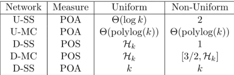
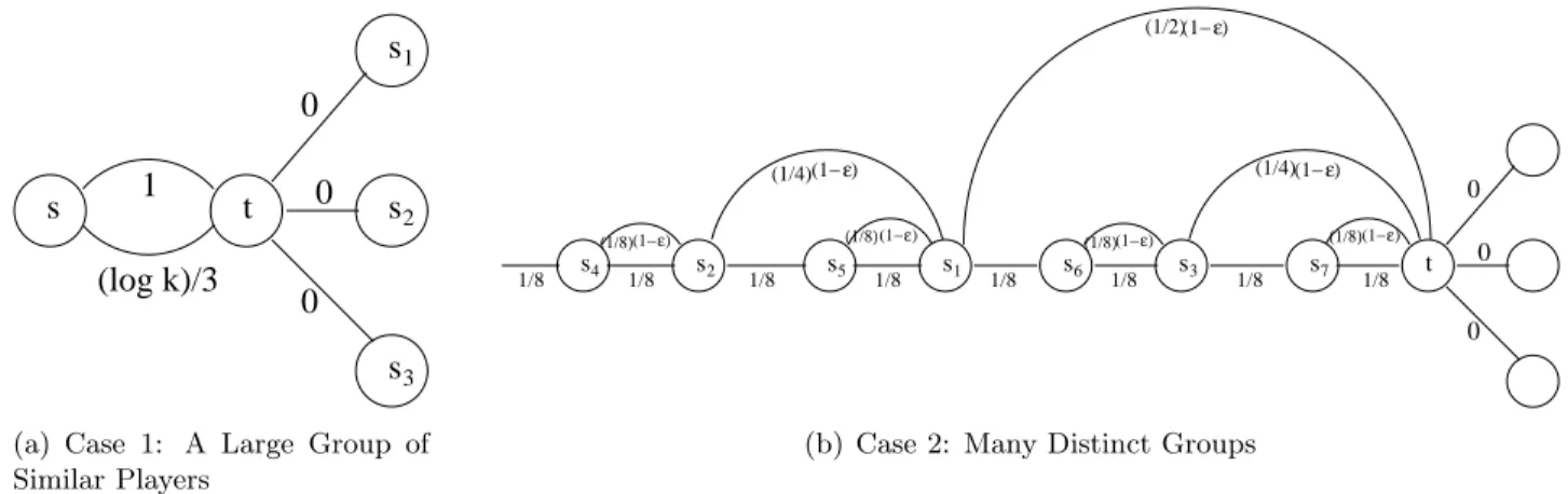
logkplayers. Budget-balance implies that there exists a player j for whichξ(j, S)≤1/logk. The Proximity Lemma (Lemma 4.10), our choice of α, and the fact that k is sufficiently large then imply that ξ(j, S) ≤ 2/logk for every j ∈ S. Create a single-sink undirected network as follows (Figure 1(a)). Each player not inS has a zero-cost edge from its source vertex to the single sink t. The players ofS share a common source vertexs, and there are two parallel edges fromstot, with costs 1 and (logk)/3. The optimal solution clearly has cost 1. On the other hand, if all players of S share the more expensive s-t edge, then each incurs a cost share strictly less than 1 and will not unilaterally deviate to the unit-cost edge. This outcome is therefore a PNE, and the POA in this network game is (logk)/3.
t s s s s 0 0 2 3 (log k)/3 1 0 1
(a) Case 1: A Large Group of Similar Players (1− )ε (1− )ε (1− )ε (1− )ε (1− )ε (1− )ε (1− )ε 0 0 0 1/8 1/8 1/8 1/8 1/8 1/8 1/8 1/8 s4 s2 s5 s1 s6 s3 s7 t (1/8) (1/4) (1/8) (1/4) (1/8) (1/8) (1/2)
(b) Case 2: Many Distinct Groups
Figure 1: Proof of Theorem 4.3. Networks that induce games with large POA for uniform protocols with many similar players and for those with many different players, respectively. In (b), the precise value of ǫis different for different edges (see text).
In the second case, there are at leastk/logkdistinct non-empty groups. Our choice ofαensures that αalog5k≥k+ 1 for a sufficiently large constant athat is independent of k. We can therefore pick one player out of every Θ(log5k) groups to obtain a set S of 2p−1 players such that: p is a
positive integer; |S| = Θ(k/log6k); and every pair j, h of distinct players of S either come from different Ai’s or have fi-values that differ by at least a (k+ 1) factor. We rename players of S so
that they are ordered according to the Ai’s, and in decreasing order of fi-values within anAi.
We next construct a single-sink undirected network (Figure 1(b)). Each player not in S again has a direct zero-cost edge tot. The rest of the network is similar to a lower bound construction for the online Steiner tree problem [28] and is defined in rounds. In the 0th round, we add a unit-cost edge (the main path) incident to t. For r = 1, . . . , p, in the rth round, we bisect the 2r−1 edges of the main path created in previous rounds with the sourcess2r−1, . . . , s2r−1 — that is, each such
edge is replaced by two edges (in series) with half the cost, with a new source vertex between them. Additionally, we create a shortcutedge between each source added in the rth round and its neighbor on the main path that is closer to t, of cost 2−r((k−1)/k)p−r+1. The cost of all of the shortcuts added in a round is Ω(1). The optimal outcome, with all players following the main path, has unit cost.
The outcome in which all players completely eschew the main path has cost Ω(p) = Ω(logk), and we complete the proof by showing that it is a PNE. Consider this outcome and a playerj using the pathPj. The first edge ofPj is the shortcut (sj, sh). Everysj-sh path other than the shortcut
comprises only edges of the main path (currently used by no players) and edges added in subsequent rounds (each currently used only by players with larger index). The claim is that player j’s cost shares on such a path would total at least a (k−1)/k fraction of the path cost, and this is no less than the cost incurred on its shortcut. To argue the claim, consider the players with which j would share edges on this sj-sh path: there are some from later groupsAi (who pay nothing inj’s
presence), and some players in the same groupAi asj but which have fi-values (relative to fi(j))
that are bounded above by a geometric sequence with ratio 1/(k+ 1). The Separation Lemma implies that the sum of the cost shares of all of these players is at most a 1/k fraction of the path cost, which implies the claim.
1+ε s1 s2 s3 sk−1 sk t 1 0 0 0
. . . .
0 0. . . .
. . . .
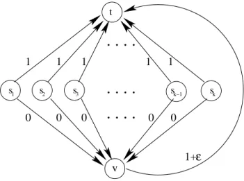
v 1 1 1 1Figure 2: Proof of Proposition 4.12. Every uniform protocol has worst-case POA at least k in directed single-sink networks.
After player j reaches sh, it shares each remaining edge of Pj with at least one player of lower
index. By the Separation Lemma, the sum of its cost shares on these edges is strictly less than 1/k, a lower bound on the cost it would incur for being the sole inhabitant of some edge on the main path. ThusPj is a best response for player j, and this outcome is a PNE.
4.2 Directed Graphs: Optimality of the Shapley Protocol
We now turn to directed networks, and prove that the Shapley cost-sharing protocol is the optimal uniform protocol. We first note that the worst-case POA is a useless measure for differentiating between competing protocols in directed networks.
Proposition 4.12 (POA in Directed Networks) For every k≥1, the worst-case POA of
ev-ery uniform protocol in k-player directed networks is k. The lower bound holds even in single-sink directed networks.
Proof: Fix k and a uniform protocol. For the upper bound, consider a directed network and the induced network cost-sharing game. Let (P1∗, . . . , Pk∗) denote an optimal outcome, with cost C∗. Every playerican guarantee itself a cost of at mostC∗, independent of the protocol and the other players’ choices, by choosing the path Pi∗. Thus in a PNE, the cost of each player is at most C∗. By budget-balance, the cost of every PNE is at mostk·C∗.
The lower bound is provided by the single-sink network shown in Figure 2. The optimal outcome has cost 1 +ǫ, where ǫ > 0 is arbitrarily small. The outcome in which each player i selects the directsi →tpath is a PNE (for any protocol) and has cost k.
Remark 4.13 Proposition 4.12 and its proof hold even fornon-uniformcost-sharing protocols (see
1+ε s1 s2 s3 sk−1 sk t 1 1/2 1/3 1/(k−1) 0 0 0 0 0 1/k
. . . .
. . . .
. . . .
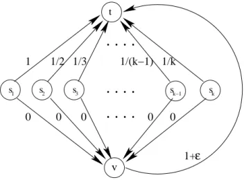
vFigure 3: Proof of Theorem 4.15. Every linear monotone protocol has worst-case POS at least Hk
in directed single-sink networks.
Proposition 4.12 also holds, with the same proof, for the worst-case reachable POA in (single-sink) directed networks. We therefore resort to our weakest inefficiency measure, the price of stability (POS). Anshelevich et al. [2] proved the following tight guarantee for the Shapley protocol.
Proposition 4.14 (POS of the Shapley Protocol [2]) For everyk≥1, the worst-case POS of
the Shapley protocol ink-player directed networks is thekth Harmonic numberHk: 1+12+· · ·+1k =
lnk+O(1).
Using the technical tools already developed in this and the previous section, we can quickly prove that the Shapley protocol is optimal.
Theorem 4.15 (Optimality of the Shapley Protocol) For every k ≥ 1, every uniform
cost-sharing protocol has a worst-case POS of at least Hk in k-player single-sink directed networks.
Proof: Fix k ≥ 1 and a uniform cost-sharing protocol for the player set {1,2, . . . , k}. By Lem-mas 4.4–4.6 and Remark 4.7, we can assume that the protocol ξ is linear. Lemma 3.10 ensures that ξ is monotone in the sense that ξ(i, S) ≥ ξ(i, T) whenever i ∈ S ⊆ T ⊆ {1, . . . , k}. Since ξ is budget-balanced, there is a player ik satisfying ξ(ik,{1,2, . . . , k}) ≥ 1/k. Similarly, for each
j=k−1, . . . ,1, there is a player ij satisfyingξ(ij,{1, . . . , k} \ {ij+1, . . . , ik})≥1/j.
Now consider the single-sink directed network of Figure 3, taken from [2]. There is a sink t, source verticess1, . . . , sk, and an additional vertexv. Playerij has sourcesj and sinkt. For eachj,
there is an edge of cost 1/jfromsj to tand an edge of zero cost fromsj to v. There is also an edge
of cost 1 +ǫ from v to t. The optimal solution has cost 1 +ǫ. On the other hand, we claim that in the network cost-sharing game induced by ξ, the only PNE has cost Hk. To see this, consider
an arbitrary outcome of the game, and let S ⊆ {1,2, . . . , k} denote the set of players that share the edge (v, t), with the rest of the players choosing their one-hop paths tot. Suppose that S6=∅ and let ij ∈S be the player ofS with maximum indexj. By construction,ξ(ij,{i1, . . . , ij})≥1/j.
ij incurs cost only 1/j by choosing the pathsj →t, this outcome cannot be a PNE. ThusS =∅in
the unique PNE, which has cost Hk.
4.3 Convergence of Better-Response Dynamics
Our final application of Theorem 3.8 is technically straightforward but conceptually interesting. Guarantees that equilibria (such as PNE) always exist in a family of games are important but lack predictive power: how do we know that rational players will successfullyreachsuch an equilibrium? A guarantee that selfish participants converge to an equilibrium through repeated experimentation is much more compelling that a mere existence result.
Better-response dynamicsis a simple and well-studied model of repeated experimentation: while the current outcome is not a PNE, choose an arbitrary player that could decrease its cost by switching paths, and update its path to a better one. If better-response dynamics is guaranteed to converge in a game, then the game obviously has at least one PNE; the converse generally fails (see e.g. [47]). But Theorem 3.8 implies a converse of sorts for network cost-sharing games: the only way to guarantee the existence of PNE in all such games is to guarantee the convergence of better-response dynamics.
Theorem 4.16 (Convergence of Better-Response Dynamics) In every network cost-sharing
game induced by a linear and uniform protocol, better-response dynamics always converges to a PNE.
Proof: First consider a potential-based protocol ξ for a player set {1,2, . . . , k}. Every network cost-sharing game induced by ξ admits a weighted potential function Φ, given in (3), and every time a player changes its path in better-response dynamics, Φ strictly decreases (4). Since there are only finitely many outcomes, better-response dynamics must terminate.
For an arbitrary linear and uniform protocol ξ, we can apply Theorem 3.8 to expressξ as the concatenation of potential-based protocols ξ1, . . . , ξm for disjoint player sets A1, . . . , Am. Players
of A1 are unaffected by the choices of other players, so the above argument can be applied to ξ1 and A1 to conclude that, in an arbitrary network cost-sharing game induced byξ, better-response dynamics eventually reaches an outcome from which no player of A1 has an incentive to switch paths. This property cannot be violated by subsequent moves by players from A2, . . . , Am, so no
player of A1 will ever change paths again. Proceeding inductively on the Ai’s, we conclude that
better-response dynamics eventually terminates.
Theorem 4.16 implies that, for linear protocols, strengthening the stability constraint (2) in Section 1.2 to require the convergence of better-response dynamics has no effect on the protocol design space.
5
Characterization of Uniform Protocols: The Proof
This section presents a proof of Theorem 3.8. The “if” direction is immediate from Propositions 3.4 and 3.7. The four major milestones of the “only if” direction are as follows.
1. Every linear and uniform protocol ξ must be monotone in the sense that ξ(i, S) ≥ ξ(i, T) whenever i∈S ⊆T ⊆ {1,2, . . . , k}. (Recall Lemma 3.10.)
2. For every linear and uniform protocol ξ, the players can be partitioned into ordered equiv-alence classes so that ξ(i, S) > 0 if and only if i belongs to the lowest-indexed class that intersects S. Different equivalence classes correspond to disjoint player sets that are com-bined via concatenation.
3. For every linear and uniform protocolξthat is also positive, all of its cost shares are uniquely determined by thek−1 pairwise cost shares ξ(1,{1,2}), ξ(1,{1,3}), . . . , ξ(1,{1, k}). 4. For every linear and uniform protocolξ that is also positive, ξ is potential-based.
We work with undirected networks throughout the proof. Our proof can be modified trivially to use only directed networks.
Our first technical lemma builds toward the first milestone of the proof by showing that any failures of monotonicity in a linear uniform protocol must be “symmetric”. The proof of this lemma also develops arguments crucial to the second milestone of the proof of Theorem 3.8 (see Lemma 5.4, below).
Lemma 5.1 Letξ be a linear and uniform cost-sharing protocol with player set{1,2, . . . , k}. LetS
be a non-empty set of players andiandj distinct players not inS, and suppose thatξ(i, S∪ {i})< ξ(i, S∪ {i, j}). Then ξ(j, S∪ {j})≤ξ(j, S∪ {i, j}).
Proof: Fixξ,i,j, andS, and assume thatξ(i, S∪{i})< ξ(i, S∪{i, j}); in particular,ξ(i, S∪{i, j})> 0. The heart of the proof is the following claim: for all positive constantsα and β, if
α(ξ(i, S∪ {i})−ξ(i, S∪ {i, j}))< β(ξ(i,{i})−ξ(i,{i, j})), (7) then
α(ξ(j, S∪ {j})−ξ(j, S∪ {i, j}))≤β(ξ(j,{j})−ξ(j,{i, j})). (8) To see why the claim implies the lemma, set β = 1. Since ξ(i,{i}) = 1 and ξ(i,{i, j}) ≤ 1, the right-hand side of (7) is non-negative. Since ξ(i, S ∪ {i}) < ξ(i, S ∪ {i, j}) by assumption, inequality (7) holds for all values of α > 0. By the claim, inequality (8) holds for every α > 0. Since the right-hand side of (8) is nonnegative, we conclude thatξ(j, S∪ {j}) ≤ξ(j, S∪ {i, j}).
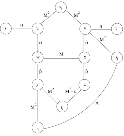
To prove the claim, fix α and β and consider the network shown in Figure 4. All players of S have sourcesand sinkt. Players outsideS∪ {i, j}are confined to a different, disjoint subnetwork. The parameterM is sufficiently large relative toα,β, and 1/ξ(i, S∪ {i, j}). The parameterA is at least M2; its precise value will be fixed later. We show that if the claim fails, then we can choose edge costs so that the game induced by ξ in this network has no PNE, thereby contradicting the stability ofξ.
We first argue that, at equilibrium, no player chooses a path containing both the edges (si, u)
and (si, v). This is true for playeribecause it must choose a simplesi-ti path. For a contradiction,
assume that at least one player of S∪ {j} chooses a path containing both these edges, and let e be one of the two edges that is not used by playeri. By budget-balance, one of the players usinge must pay at least M2/k for it. No player of S will incur such a large cost share at equilibrium because of the deviations→u→ w→x→v→t(assumingM is sufficiently large). Player j will not incur such a cost share at equilibrium, because thew-v subpath of its path that contains ecan be replaced by the subpathv→x→w (removing the resulting cycles if necessary) to decrease its cost. Thus no player will use edgeein a PNE.
s s s t t u v t w x y z M M M M M A 0 0 2 2 2 M2 2 M −2 ε i i j j α α β β
Figure 4: Network in the proofs of Lemmas 5.1 and 5.4.
A similar argument shows that no player will use the edges (y, ti) and (z, ti) in a PNE. Thus
no player other thaniuses an edge incident to si orti in a PNE. So, player j uses either the path
sj →v→x→ w→y→tj (denotedQ1) or the one-hop pathsj →tj (denotedQ2) in a PNE. Next we argue that no player of S∪ {i} uses the edge (sj, tj) in a PNE. Player j uses at most
two of the three edges (tj, y), (sj, tj), and (v, sj). If any players of S∪ {i} use the edge (sj, tj),
one of them incurs a cost share of at least M2/k for one of these three edges. (Recall thatA is at leastM2.) As above, no player ofS will incur such a large cost share in a PNE. If player iincurs a cost share of at leastM2/k on these edges, then its overall cost is at leastM2(2 + 1/k) (since no players other than iuse edges incident to si orti). Since player ican guarantee itself a cost of at
most 2M2+α+β, this cannot occur in a PNE providedM is sufficiently large.
Summarizing, player j will take path Q1 orQ2 in a PNE, and all players of S will follow the path s → u → w → x → v → t. Let P1 and P2 denote the si-ti paths si → u → w → y → ti
and si → v → x → z → ti, respectively. If player j chooses path Q1, then our assumption that ξ(i, S ∪ {i, j}) > 0 implies that player i will not use the edge (w, x) in a PNE (assuming M is sufficiently large) and hence usesP1 or P2. If player j chooses path Q2, then the cost incurred by player ion pathP2 is no more than that on any other si-ti path. Thus, if there is a PNE, there is
one in which player ichooses either P1 or P2. We label the four candidates for a PNE according to the paths selected by players iand j, and proceed to choose parameters to rule them out.
We have cj(P1, Q2) =cj(P2, Q2) =A, and ci(P1, Q1) = 2M2+αξ(i, S∪ {i}) +βξ(i,{i, j}); ci(P2, Q1) = 2M2+αξ(i, S∪ {i, j}) +β−ǫ; ci(P1, Q2) = 2M2+αξ(i, S∪ {i}) +β; ci(P2, Q2) = 2M2+αξ(i, S∪ {i}) +β−ǫ; cj(P1, Q1) = 2M2+M ξ(j,{S∪ {j}) +αξ(j, S∪ {j}) +βξ(j,{i, j}); cj(P2, Q1) = 2M2+M ξ(j,{S∪ {j}) +αξ(j, S∪ {i, j}) +β.
If (7) holds but (8) fails andǫis sufficiently small, thenci(P1, Q1)< ci(P2, Q1). Setting the cost of edge (sj, tj) to be a numberAsatisfyingcj(P2, Q1)< A < cj(P1, Q1), we obtain a network game induced by ξ with no PNE: player i wants to deviate from (P2, Q1) and (P1, Q2), while player j wants to deviate from (P1, Q1) and (P2, Q2). (Note that A ≥M2, as required.) This contradicts the stability of ξ, completing the proof.
The next lemma is a restatement of Lemma 3.10, and establishes the monotonicity of linear uniform protocols.
Lemma 5.2 (Monotonicity of Linear Uniform Protocols) Every linear and uniform
proto-col ξ for a player set {1, . . . , k} is monotone: for everyS ⊆ T ⊆ {1, . . . , k} and i ∈S, ξ(i, S) ≥ ξ(i, T).
Proof: We show ifξ is linear and uniform but not monotone, then it is not stable (a contradiction). By definition, ifξ is not monotone, there is a set S⊆ {1, . . . , k} and a pairi, i′ ∈S of players such thatξ(i, S\{i′})< ξ(i, S). This can only occur ifScontains a player other thani, i′. Among all such sets, choose one of minimum-possible cardinality. We assume henceforth thatξ(i′, S\{i})≤ξ(i′, S) as well; otherwise, by Lemma 5.1, the proof is complete.
Since the cost-sharing method ξ is budget-balanced, we have
X j∈S\{i} ξ(j, S\ {i}) + X j∈S\{i′} ξ(j, S\ {i′}) = 2 =X j∈S ξ(j, S) + X j∈S\{i,i′} ξ(j, S\ {i, i′}). Thus, ξ(i, S) +ξ(i′, S) + X j∈S\{i,i′} ξ(j, S) +ξ(j, S\ {i, i′}) = ξ(i, S\ {i′}) +ξ(i′, S\ {i}) + X j∈S\{i,i′} ξ(j, S\ {i}) +ξ(j, S\ {i′}) .
Since ξ(i, S\ {i′})< ξ(i, S) and ξ(i′, S\ {i})≤ξ(i′, S), there is a player j∈S\ {i, i′}with ξ(j, S) +ξ(j, S\ {i, i′})< ξ(j, S\ {i}) +ξ(j, S\ {i′}).
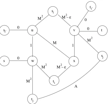
Now consider the network shown in Figure 5. All players ofS\{i, i′, j}have sourcesand sinkt. As in the proof of Lemma 5.1, players outside of S are confined elsewhere. The parameter M is a
M −2 ε M −2 ε s s u v t M 0 2 M2 i j t t M M2 2 i j A s 0 s 0 0 w x ti’ i’ M 1 1
Figure 5: Network in the proof of Lemma 5.2.
sufficiently large function ofξ(i, S). (By assumption,ξ(i, S) > ξ(i, S\ {i′})≥0.) The parameterǫ is small enough so thatξ(i, S\ {i′}) + 2ǫ < ξ(i, S). The parameterA is chosen to satisfy
2M2+M ξ(j, S\{i})+ξ(j, S)+ξ(j, S\{i, i′})< A <2M2+M ξ(j, S\{i})+ξ(j, S\{i})+ξ(j, S\{i′}). (9) We claim that the network cost-sharing game induced byξ in this network admits no PNE.
First, note that player i can guarantee itself a cost share of at most 2M2 + 1; player j a cost share of at most 2M2+M+ 2; and all other players a collective cost share of at mostM+ 2. Hence, in every PNE, the total cost incurred by all players is strictly less than 5M2−2ǫ(provided M is sufficiently large). Every outcome in which both edges incident to si or both edges incident to ti
are used by some player has cost at least 5M2−2ǫ—player imust use one edge incident to each of si and ti, and player j must incur cost at least 2M2 on the edges (sj, v), (sj, tj), and (w, tj)—and
thus none of these are PNE. By similar reasoning, no player other than j uses the edge (sj, tj) in
a PNE.
We have established the following for every PNE: player i′ must take the paths
i′ →u→ x→
v → ti′; players of S\ {i, i′, j} must take the path s→ w→ u →x → v → t; and player j must
take either the pathQ1, defined assj →v→x→u→w→tj, or the one-hop pathQ2 from sj to
tj.
LetP1 denote the pathsi→u→w→ti andP2 the path si →v→x→ti. The following four
statements will complete the proof: