Office Rent Determinants: A Hedonic Panel Analysis

(1)

MPRA

Munich Personal RePEc Archive

Office Rent Determinants: A Hedonic

Panel Analysis

Fuerst, Franz

University of Reading, Henley Business School

October 2007

Online at

http://mpra.ub.uni-muenchen.de/11445/

(2)

Electronic copy available at: http://ssrn.com/abstract=1022828

WORKING PAPER

Office rent determinants: a hedonic panel analysis

Franz Fuerst

Department of Real Estate & Planning Business School

University of Reading Reading RG6 6AW United Kingdom

(3)

Electronic copy available at: http://ssrn.com/abstract=1022828 Office Rent Determinants: A Hedonic Panel Analysis

It has been frequently observed that office markets are subject to particularly high fluctuations in rents and vacancy levels, thus exposing real estate investors to considerable risk regarding expected future income streams. This paper tries to analyze the determinants of office rents and their variability over time and across submarkets of a city in order to gain additional empirical insights into the rent price formation process.

1. Introduction

The determining factors of office rental rates are well researched and documented in a host of empirical studies. The existing research literature converges on a number of relevant factors to explain the variation in office rental rates such as age and size of the property as well as accessibility by various modes of transportation. The relevance of these factors appears to be almost universally acknowledged in the empirical literature. Commercial real estate markets, however, are characterized by spatial constraints, extensive product differentiation and information asymmetries that give rise to economically fragmented markets. A number of previous studies have demonstrated that such distinct submarkets do exist within urban office markets. The highly localized patterns of occupancy and rental rate determination found in these studies are indicative of market fragmentation. The question of market fragmentation is of immediate relevance for rental rate determinants. If markets are fragmented, office rents are highly likely to be determined by heterogeneous pricing schemes. Therefore, two identical properties would yield different rental rates if they are located in two different submarkets.

Similarly, the relative weight of rent determinants may change over time favoring buildings with certain features over others depending on the position in the real estate cycle. To date, very few studies have sought to systematically analyze the stability of office rent determinants. A closer examination of their spatio-temporal variability appears therefore warranted.

(4)

The remainder of this chapter is organized as follows. The first section reviews previous studies on spatial differentiation and cyclical fluctuations of commercial real estate markets. Next, the volatility of the Manhattan office market is examined using descriptive statistics. In a further step, I test if variables reflecting individual characteristics of buildings such as average age, density and accessibility are able to explain the variation in rental rates. Next, I test the significance of various characteristics in different phases of the market cycle using a hedonic model. The stability of parameters is analyzed cross-sectionally to test the independence of submarket observations. Instead of applying a classical fixed-effects model, hedonic regressions are estimated separately for each time period and submarket. In order to take the analysis one step further, full panel data models (Arellano-Bond models, random effects models) are estimated and the results of both the OLS estimation and the panel data analysis are discussed. Finally, I discuss the implications of the empirical results.

2. Relevant background

There exists a host of studies on the relevance of the intrametropolitan level-data in explaining the functional structure and development of office markets (Clapp 1980; Ihlanfeldt and Raper, 1990; Mills 1990; Hanink 1997; Bollinger et al. 1998). These studies, however, typically neglect the dynamic time-series aspect of the data. Conversely, most of the time-series research on real estate market cycles is aspatial in that it assumes a simultaneous adjustment of all intraurban locations to changing supply and demand relations at the metropolitan level. Hence, very few studies seek to combine cross-sectional and time series office market data at the intra-urban level (Mourouzi-Sivitanidou 2002).

Market efficiency

In general, all empirical models take one of the two possible positions: 1) The metropolitan area forms a unitary real estate market and 2) submarkets within a city are fragmented and in many cases out-of-sync with the overall development of a metropolitan area. The first research tradition bases its assumptions on urban location theory which implies that the relative price differences between intra-urban submarkets remain stable over time irrespective of cyclical oscillations in absolute prices (constant ratio

(5)

hypothesis). This stability is ascribed to the high degree of intraurban mobility of office tenants, a high price elasticity of demand and possibilities to arbitrate in a situation of mispricing (DiPasquale and Wheaton 1996). Following this theory, a change in the relative price hierarchy of an urban market is only possible if major changes in either the physical attributes of particular locations or in transportation and communication technologies occur.

If, however, one assumes a less than fully efficient market, office buildings turn out not to be close substitutes for each other and information asymmetries cause the market to split up into several functional or spatial submarkets (Evans 1995). Empirical studies supporting this hypothesis also point out that the increasing functional specialization of spatial submarkets has resulted in additional economic fragmentation of markets (Sivitanidou 1995, 1996, Bollinger et al. 1998). In a further study of the housing market, Can (1996) examined the presence of spatial segmentation, as reflected in heterogeneous pricing schemes. She contends that if neighborhood effects enter as direct determinants of housing prices, such as a premium, then one can assume a uniform housing market under investigation, since there will be one price schedule. In contrast, if neighborhood differentials lead to varying attribute prices, one can assume the presence of independent price schedules, thus the existence of a spatially segmented market.

Do submarkets matter?

Numerous empirical studies have shown that an elaborate functional division of labor exists indeed between various submarkets in a metropolitan area. This functional specialization which may give rise to fragmented submarkets is reflected in the spatial organization patterns of office firms, such as front office – back office divisions and industry clusters in particular areas of a city (Shilton 1999, Schwartz 1992, Hanink 1997, Sivitanidou 1996). It is thus pertinent for commercial real estate analysis to devise methods that are capable of capturing the cross-sectional and time-series dynamics of rent determining factors. In this context, one promising approach is panel data analysis, which is applied in this study along with OLS hedonic regression models.

(6)

In their seminal study of the constancy of rent variations and the robustness of coefficient estimates, Glascock, Kim and Sirmans (1993) apply random effects and heteroskedastic autroregressive models. The authors find that the coefficients vary across time, location and class of building. They also conclude that random-effects models are superior over fixed-effects methodologies. The present study also applies a random-effects model and compares the results to the OLS regression analysis. In an empirical study of the Orlando office market, Archer (1997) found that there is at least limited evidence of a transitory and in some cases even permanent segmentation of submarkets. Moreover, he finds that segmentation of submarkets is continuous rather than divided by sharp boundaries. Slade (2000) estimated rent determinants during market decline and recovery but did not include any explicitly spatial variables in his study. Dolde and Tirtiroglu (1997) included submarkets in their analysis and found distinct patterns of temporal and spatial diffusion of real estate prices using GARCH-M methods. The present study revisits the question of spatiotemporal stability by analyzing the coefficients of rent determinants in a hedonic OLS and random-effects framework.

Rent determinants

The following section gives an overview of the most important rent determinants identified in previous empirical studies. Most of these studies apply a hedonic model to test the relative importance and order of these factors.

Vacancy levels are among the most important drivers of rental rate formation in the existing research literature. Sirmans, Sirmans and Benjamin (1989) find an the inverse relationship between vacancy rates and rents for apartment buildings and Sirmans and Guidry (1993) confirm these results for retail rents. Studies of office rent determinants, such as Clapp (1993) and Mills (1992) also find this variable to be highly significant in their respective empirical studies. In general, vacancy rates may be interpreted as a proxy for the general attractiveness of a building. This hypothetical relationship is transmitted in practice by the behavior of landlords who tend to lower asking rents in response to rising vacancy in a building in order to attract new tenants.

(7)

The rentable building area of a given property is a proxy for increased opportunity for to-face interaction within a large building. Clapp (1980) confirms the value of face-to-face contact in management decisions. More recent studies have shown that the value of face-to-face communication persists despite widespread availability of information and communication technology (Gat 1998). Apart from this, large tenants are typically willing to pay a rent premium for sizable units of contiguous office space (10,000 square feet and above) that enable their internal operations to run more smoothly than a situation with several scattered locations. Thus, Bollinger, Ihlanfeldt, and Bowes (1998) find average floor area to be a significant variable in determining rents in the Atlanta office market, most likely for the same reason.

Building age shows up significant in a host of studies on office market rent determinants (Bollinger, Ihlanfeldt and Bowes 1998, Slade 2000, Dunse et al 2003). In this study, building age is expressed as year built so that a more recent construction date has a positive impact on rental rates. In case a property underwent major renovation, the original construction date is replaced by the renovation completion date. The age of a building is typically a proxy for the quality of the technological infrastructure and adequacy of the floor layout.

The number of stories of a building represents more sophisticated elevator systems in tall buildings, the availability of panoramic views and a potential landmark status for very tall buildings. Shilton and Zaccaria (1994) found a convex relationship of building height in an earlier study of the Manhattan office market,

Amenities and in-house services are included in many hedonic studies of office rents. Ho et al (2005) report that functionality, services, access and circulation, presentation, management and overall amenities are the order of importance in assessing office building quality. The amenities variable used in this study is a compound measure of the availability of up to 34 building amenities, including banking, mailing, medical, retail and hotel facilities in the building as well as onsite facility management, availability of large trading floors, showrooms, courtyards, fitness clubs and atriums, subway access on premises, waterfront location, and onsite management. It is expected that tenants pay a

(8)

premium for convenient access to these amenities which is confirmed in the significance levels of this variable throughout the estimated period.

Turning to location-specific price determinants, a number of variables were included in the hedonic model used in this study. The importance of spatial variables in hedonic modeling is almost universally acknowledged in the literature. The broad variety and potential cross-influence of spatial variables poses some intricate methodological problems, however. The goal of hedonic modeling should be to maximize the efficiency of the estimators while minimizing information loss due to elimination of important variables in an effort to reduce multicollinearity. In an effort to categorize spatial variables, Can (1996) proposed to distinguish between adjacency and neighborhood effects. Adjacency effects which are externalities and spillover effects due to the geographic position of a property relative to other points of reference (i.e. other properties, transportation infrastructure) can be captured by geostatistical methods and various accessibility measures. Neighborhood effects, which are distinct perceived or observable characteristics of an area, also have an impact upon property prices and rental rates although their contribution to price formation is more difficult to measure.

Access to commercial centers is included in various forms in hedonic studies of office rents (see Sivitanidou 1995). In a study of Atlanta office rents, Bollinger, Ihlanfeldt and Bowes (1998) find that proximity to concentrations of office workers exert a positive impact on rent levels. In general, this variable reflects ease of access to clients and business services in the immediate vicinity of the building. In the present study, this variable is operationalized as the average distance to the 20 closest office buildings and is calculated with a nearest neighbor algorithm in a Geographic Information System. The inverse of the distances calculated for each building distance pair is weighted by the square footage of the neighboring building and entered into the model. Therefore a positive sign is expected for the coefficients to the extent that larger square footage and shorter distances yield higher values. Similarly, the amount of office space located within 1500 feet of an office building indicates whether a building is located in a major office cluster. Therefore, a positive impact of this variable is expected. Rosenthal and Strange (2001) found evidence that such knowledge spillovers operate almost exclusively at the

(9)

small-scale level. The authors conclude from their observations that such spillovers evaporate rapidly across space.

The distance to the nearest subway station measures ease of access to public transit network. Cervero and Duncan (2002) found that office properties located close to a public transit public transit stations command higher prices per unit in the order of 120 percent for commercial land in a business district within a quarter mile of a commuter rail station. Although very few office buildings in Manhattan are located outside a radius of this size, this variable is included to test whether even smaller differences in average distance to mass transit stations have an impact on rental rates.

Finally, the latitude and longitude coordinates of a property are included in various

hedonic models. While not meaningful per se, these variables are potentially capable of capturing spatial effects not operationalized in the other variables of the model as the coefficients of these variables are allowed to vary parametrically over space. This approach was developed and applied in a number of previous studies such as Can and Megbolugbe (1997), Casetti (1997) and Clapp (2003, 2004).

3. Methodology

In the first step of the empirical analysis, some basic descriptive measures are used to investigate volatility and cross-sectional variability of rental rates. To explore potential lags in the adjustment of submarkets to changing market conditions, cross-correlation measures will be examined.

Hedonic analysis

Hedonic regression modeling has become the standard methodology for examining price determinants in real estate research. The quintessential log-linear hedonic rent model is specified in the following form:

i i i i i

x

Z

R

=

α

+

β

+

φ

+

ε

ln

(1)

(10)

Where Ri is asking rent per square foot in dollars for a given office building, xi is a vector

of the natural log of several explanatory locational and physical characteristics, β and φ

are the respective vectors of parameters to be estimated. Zi is a vector of time-related

variables and

ε

i is a random error and stochastic disturbance term that is expected to

take the form of a normal distribution with a mean of zero and a variance of σe

2 . The hedonic weights assigned to each variable are equivalent to this characteristic’s overall contribution to the rental price (Rosen 1984).

Rent determinants can be roughly grouped into neighborhood/building-specific and accessibility/location factors (see for example Des Rosiers et al 2000) For the purpose of this study, I specify two hedonic models. While Model I captures building-specific factors, Model II contains locational attributes. The final specification of Model I used to estimate the empirical results reported below is:

(Model I)

ln

R

_i

=

α

_i

+

β

₁

ln

V

_i

+

β

₂

ln

B

_i

+

β

₃

ln

T

_i

+

β

₄

ln

S

_i

+

β

₅

ln

A

_i

+

ε

_i (2)

where Vi represents the vacancy rate of a building, Bi is the rentable building area in

square feet, Ti indicates the year of construction or major renovation, Si is the number of

stories and Ai is a vector of in-house amenities. Model II was specified as follows:

(Model II)

ln

R

_i

=

α

_i

+

β

₆

ln

D

_i

+

β

₇

ln

F

_i

+

β

₈

ln

M

_i

+

β

₉

ln

N

_i

+

β

₁₀

ln

W

_i

+

ε

_i (3)

where Di represents the inverse of the distance of the twenty office buildings with the

shortest distance to the property in question (weighted by their square footage), Fi is the

amount of square feet of office space within a distance of 1500 feet, Mi is the distance to

the nearest subway station and Ni and Wi are the longitude and latitude coordinates of the

property.

To detect differences in the weight of parameter estimates across submarkets, a standard fixed effects model can be estimated (Hsiao 2003):

(11)

i i nit n it it it

x

R

=

α

δ

+

α

δ

+

...

α

δ

+

β

+

ε

ln

₁ ₁ ₂ ₂ (4)

In this model, the incidental parameters

α

_i are fixed constants and

δ

_jitis a

submarket-specific indicator (dummy variable). This Least Squares Dummy Variable (LSDV) model can be used to detect both longitudinal and cross-sectional heterogeneity. The drawback of the LSDV model is, however, that it only allows intercepts to differ across space while assuming constant variable coefficients. Thus, instead of estimating a single LSDV model, it is more appropriate to estimate the full hedonic model separately for each submarket and time period when investigating the time-series cross-sectional variability of rent determinants. Alternatively, a full random-effect panel model can be estimated as outlined in the following section.

Random-effects panel data estimation

In order to expand the scope of the hedonic framework by simultaneously analyzing the longitudinal and cross-sectional components of the data, a panel regression model is introduced. The fixed-effects model as outlined in the previous section assumes that differences across units of observation are captured by differences in the constant term.

(5)

A fixed effects model estimation is limited, however, by the fact that this model assumes

the intercepts

α

i are fixed, estimable parameters so that individual effects cannot be

captured with this approach. The random effects model assumes that the observations are random draws from the same distribution and therefore part of a composite error term of the following form:

(6)

where

u

i is a group-specific random element which captures unobserved

property-specific factors. In the random effects model all three components (intercept, time-specific and cross-sectional error components) are assumed random and not fixed. The

it i it it

x

R

=

β

+

α

+

ε

ln

it i i it it

x

R

=

β

+

α

+

µ

+

ε

ln

(12)

prerequisite for applying a random-effects model is, however, that this unobserved

heterogeneity be normally distributed and uncorrelated with the explanatory variables Xit.

The main advantage of this approach is that the number of parameters to be estimated is substantially reduced compared to a fixed-effects approach or any repeated-measurement sequential estimation. Especially when there is serial correlation of the composite error term, the random effects GLS approach yields superior results compared to the OLS and fixed effects approach.

In a time-series estimation of rental rate determinants, it appears reasonable to assume that one of the more important determinants is the rental rate of the past period. Inclusion of lagged values of the dependent variable is problematic, however, because these values are typically correlated with the residuals. Therefore, the lagged dependent variable must be instrumented. Arellano and Bond (1991) and Arellano and Bover (1995) developed an estimation approach that solves this problem.

Parameters are estimated by assuming that future error terms do not affect current

values of the explanatory variables and that the error term

ε

it is serially uncorrelated. It is

also assumed that changes in the explanatory variables are uncorrelated with the unobserved property-specific and/or subarea-specific effects. This set of assumptions generates moment conditions that allow estimation of the relevant parameters. The instruments corresponding to these moment conditions are appropriately lagged values of both levels and differences of the explanatory and dependent variables. A frequent problem with this type of estimation is that the moment conditions tend to overidentify the regression model, which can be diagnosed using the Sargan test for overidentifying restrictions. A second important diagnostic test is the Arellano-Bond test for autocovariance of the residuals. While the presence of first-order autocovariance does not preclude that the estimators of the hedonic model are consistent and efficient, the presence of second-order autocovariance would be a clear sign of misspecification (Arellano-Bond 1991, 281-2).

(13)

Testing for longitudinal and cross-sectional structural change

Based on Slade's (2000) proposition that market participants value physical, rental and locational characteristics of a building differently during distinct phases of the market cycle, I estimate the parameters of both model specifications for each quarter from 1999 through 2004 individually and compare the resulting parameter estimates over time. Each of the quarterly estimates is assigned to one of three periods in the market cycle that occurred during the observed period: (1) market recovery, (2) peak, and (3) decline. I then test for cross-sectional parameter stability of the hedonic estimates across submarkets in the next step. Under the assumption of an efficient market with a city-wide unified pricing scheme, the expectation is that the coefficients of the hedonic characteristics be equal in all areas. This is expressed by the null hypothesis:

H0: β1 = β1r =β1p = β1d;

β2 = β2r = β2p = β2r;

…

βn = βnr = βnp = βnd

against the alternative

Ha: H0 is not true

In this notation the coefficients βn are the parameter estimates of a particular variable

with the second subscript denoting the respective phase of the market cycle (r= recovery, p=peak, d=decline). A Chow test can be applied to determine whether the set of regression parameters is equal across groups (Chow 1960):

)) 1 ( 2 /( ) ( ) 1 /( ) ( + − + − − − − = k m n RSS RSS R RSS RSS RSS F j i j i p CHOW (7)

where RSSp is the residual sum of squares of the pooled regression model, i and j are the

two subsamples to be compared, and n and m are the number of observations in the

(14)

null hypothesis of structural stability of hedonic regression parameters and accept the alternative hypothesis of structural heterogeneity.

In the cross-sectional analysis, the hedonic regressions for each of the three quality classes (A,B,C) are estimated separately and the results are compared to one another. Hence, accepting the alternative hypothesis would provide evidence of heterogeneous pricing schemes. Besides the Chow test, the Tiao-Goldberger F-statistic is computed to test for individual parameter stability.

The Tiao-Goldberger test is an F-test of the following form:

1 ) ( ) ˆ ( 1 1 2 1 − − × − =

∑

= = = L K T SSR b b F j L j j L j j j L j ij TG (8) with

∑

= = = _L j ij L j ij ij P P b b 1 1 1 ˆ

where L is the number of models, bˆij are the OLS estimates of the ith parameter in the jth

independent model, Pij is the diagonal element for the ith parameter of (X’X)j-1, SSRj the

sum of squared residuals for the jth model; Tj the number of observations used to

estimate the jth model and Kj the number of parameters in the jth model. Alternatively,

the Chow and Tiao-Goldberger test statistics can be calculated by including an interaction term in a General Linear Model (GLM) framework. The GLM pools the sums of squares and

degrees of freedom for submarkets and submarkets times the independent variable (X) in

question and reports the F-test value. Computed separately for each of the variables, the resulting F test values indicate parameter stability of each of the variables used in the regression.

In the next step, hypothesis test outlined above is applied to time-series observations. Under the assumption of an efficient market with a unified pricing scheme, we expect the

(15)

coefficients of the hedonic characteristics to be equal in all time periods. We reject the null hypothesis of equal coefficients if the test statistics reveal that the coefficients differ significantly at various points of the market cycle.

Defining the phases of the market cycle

In order to test the implications of quarterly parameter estimates for the cyclical development of the market, it is necessary to first identify the phases and turning points of the market cycle. This is typically achieved by estimating a general trend around which cyclical fluctuations occur. There exist several econometric tools, most notably the Hodrick-Prescott filter, for detrending time series data. The present study does not follow this methodological strand of defining turning phases in that no effort is made to determine time series trends and/or hypothetical long-term equilibria. Instead, phases are defined based on the sign and strength of rental rate growth rates over a minimum duration of four quarters. Other applications of this method can be found in Mintz (1969), Watson (1994), Artis, Kontolemis and Osborn (1997), Mueller (1999) and more recently in Krystaloggiani, Matysiak and Tsolacos (2004).

The time series data analyzed in this study –albeit rather short for detecting generalizable patterns- lends itself particularly well for the study of real estate market cycles since the individual phases are clearly discernable with practically no ambiguous periods or 'noisy' oscillations. Consequently, no smoothing methods have to be applied prior to defining the start and end points of cycle phases. The five-year rental rate time series of Manhattan exhibits three distinct phases of the cycle: recovery, peak and decline. Each dataset in the quarterly series is assigned to one of the three phases that occurred within the observed time span by applying three simple rules.

If

∆

R

_t₋₂

∧

∆

R

_t₋₁

∧

∆

R

_t

>

0

, Phase = recovery

If

∆

R

t−2

∧

∆

R

t−1

∧

∆

R

t

<

0

, Phase = decline

(16)

Put differently, periods of positive growth of rental rates for more than three quarters are identified as part of the recovery phase while negative rental rate growth for more than three quarters is considered to mark the decline phase of the market. The peak phase includes the three consecutive quarters with the highest absolute rental rates in the time series. Additionally, the maximum point is also defined as the turning point from positive growth (recovery) to contraction (decline) to make sure that the sequence of the phases is recovery-peak-decline. Figure 1 contains an illustration of the timeline of the three cycles.

Figure 1: Phases of the Manhattan office market cycle

Recovery Q1-1999 through Q2-2000

Peak Q3-2000 through Q1-2001

Decline Q2-20001 through Q2-2004

(17)

4. Data issues

The empirical estimation of the model is drawn from the CoStar property information system which covers the Manhattan office market almost completely on a building-to-building basis. The time increment used in this model is one quarter, which is different from most other modeling studies which use either annual or semi-annual data. Quarterly data are typically subject to greater fluctuations than annual or semi-annual averages. The longer time-intervals eliminate a large part of the variation of more fine-grained data which contains important information on dynamic adjustment mechanisms of the market. Although the time-series of building data was relatively short (22 quarterly observations in 6 years), three distinct phases of the real estate market cycle could be identified during this period. To put this relatively short period in perspective, the two subsequent figures demonstrate the longer term development of rental rates in Manhattan and its major subdivisions. Figure 2 illustrates the trajectory of quarterly Manhattan rental rates from 1980 through 2004. Figure 3 shows rental rates broken down by subarea from 1992 through 2004.

(18)

Figure 3: Longer-term index of Manhattan real rental rates (Q1-1980=100) Data: Real Estate Board of New York, Grubb & Ellis

Inventory, occupancy and vacancy data

Quarterly building data were obtained from CoStar spanning a period of about six years. The sample contains data on location, building area, story height, asking rents, vacancy rates, sublet space as well as other building characteristics. The entire sample contains 492 million square feet of office space and nearly 3,000 Manhattan office buildings. While this database contains practically all Manhattan office buildings with more than 10,000 square feet, only 870 to 950 buildings (depending on the time period and number of variables included in the specification) of the full sample could be used for the purpose of the hedonic analysis due to missing data for most of the smaller office buildings. While six years or 16 quarterly observations constitute a rather short time series, three typical phases of the real estate market cycle are contained within them. Moreover, longer time-series hedonics typically face the problem of controlling for the effect of new product being introduced into the market while the obsolete stock is being phased out (Hulten

(19)

2003). While this heterogeneity of the analyzed sample potentially hampers comparability over time, changes in the composition of office inventory due to new construction and demolition are below one percent and thus not critical for the longitudinal comparability of parameter estimates.

Rental data

The data on rent used in this study are asking rents per square foot aggregated from a large sample of buildings in the CoStar property information system. Asking rents, as opposed to actual rents which are based on lease transactions, are known to be inaccurate. Assuming that the error is systematic but not fixed, the differences between asking and actual rents vary with the position in the market cycle. For instance, it can be assumed that the difference between asking rents and actual rents will be highest immediately at the outset of a recession. This is due to the fact that landlords are reluctant to lower asking rents after a prolonged period of growth but will instead concede free rent periods and other incentives to prospective tenants. Only when market conditions have deteriorated considerably and vacant space becomes a serious problem, landlords will adaptively discount asking rents in order to attract tenants. While rents based on actual leases would be preferable, they are generally not available to researchers and pose additional problems, such as the adequate incorporation of non-monetary or non-rent-related incentives in the lease. In the absence of actual rents, asking rents are being used in this study despite their known inaccuracies and shortcomings. The asking rents and all other monetary variables are adjusted for inflation with the implicit price deflator as applied in the National Income and Product Accounts (NIPA).

Accessibility data

A number of accessibility measures were calculated to capture spatial variables at the submarket and building level. All buildings in the database provided by CoStar were geocoded using a Geographic Information System. After assigning x and y coordinates to each building, the distance between each building and the closest subway station was calculated (see Figure 4 for a visualization of the geocoded buildings). As a measure of regional accessibility, the distance from each building to the three major public transit

(20)

hubs Grand Central Station, Penn Station and the World Trade Center PATH Station was calculated. Moreover, the distance from each office building to the closest office buildings was calculated using a nearest neighbor algorithm. To capture the opportunity of face-to-face interaction within walking distance, the amount of square feet of office space within a distance of 1500 feet was calculated. Instead of using straight line distances, so-called Manhattan distances were used which take into account the grid structure of the case study area.

Class A/B/C categorization

Although the A,B,C distinction of buildings is mainly used in industry market reports to describe the development of the three quality segments of the markets, it also proved to be useful and significant in a number of previous academic studies. Archer and Smith (2003) present a model of industry economies of scale for Class A space and tenants and introduce a working definition whereby Class A office space is characterized by a lesser degree of sensitivity to rental expenses and a higher relevance of image and prestige factors of tenants compared to the Class B and C categories. CoStar (2007) defines Class A as investment-grade properties that are well located and provide efficient tenant layouts and floor plans, have above-average maintenance and management as well as the best quality materials and workmanship in their trim and interior fittings. Class B buildings offer functional space without special attractions, and have ordinary design, if new or fairly new; good to excellent design if an older non-landmark building. These buildings typically have average to good maintenance, management and tenants. Class C comprises older buildings that offer basic space and command lower rents or sale prices. Such buildings typically have below-average maintenance and management, and could have mixed or low tenant prestige, inferior elevators, and/or mechanical/electrical systems. These buildings lack prestige and must depend chiefly on a lower price to attract tenants and investors.

(21)

20

Figure 4: Spatial distribution of office space in Manhattan (snapshot of geocoded properties). Data: CoStar Group

(22)

21

Study area

The Manhattan office market is characterized by a number of distinctive features. It is by far the largest agglomeration of office space in the United States - more than twice as large as Chicago. Second, growth rates of office employment and demand for office space are on average low compared to younger markets in Southern and Western regions. Nevertheless, Manhattan exhibits a unique concentration of financial services firms and is one of the most important financial centers in the world. About 80 percent of New York City's office space is concentrated in Manhattan. The market suffered a significant shock by the destruction of 14.5 million square feet of office space on September 11, 2001.

Despite these unique features, Manhattan is an ideal case study for exploring submarket fragmentation and small-scale locational dynamics. It has a large number of specialized sub-centers such as the Wall Street area and the Insurance District with large industry clusters. Regarding the inventory of office buildings, the market exhibits a great degree of heterogeneity regarding the vintage, size, technology and amenities of buildings. Because of the high density and maturity of Manhattan, submarkets with distinctly different supply and demand characteristics can be found within a relatively short distance from one another.

For the purpose of real estate market studies, Manhattan is commonly divided into three subareas (Midtown Core, Midtown South and Downtown). Each of these subareas is further subdivided into submarket areas.

5. Empirical Results

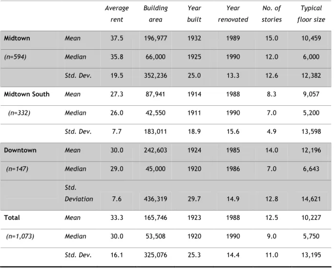
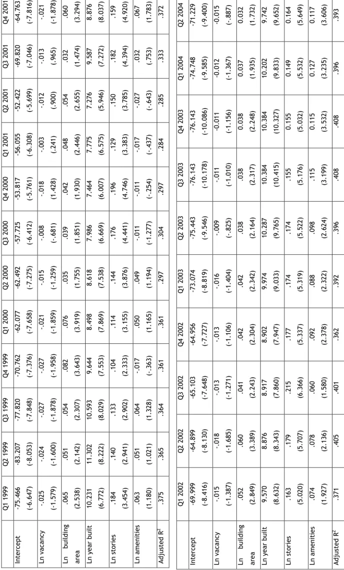
In the first step, hedonic regressions are estimated based on the Manhattan office property database described in the previous section. Table 1 shows descriptives of the variables included in the final specifications. As mentioned above, two separate models were estimated in this study. A log-linear specification was found to perform best in all regressions reported here. Table 2 shows the results of the quarterly estimation for the building-specific model (Model I). As expected,

(23)

22

vacancy levels of a building have a negative impact on rents although this variable does not reach the desired significance level in all cases. In contrast, the rentable area of a building exerts a positive impact on rent levels. The variable 'year built', which reflects either the construction date or year of major renovation shows a particularly strong impact and is highly significant. Although building age was reported as a relevant factor in most hedonic studies, it is remarkable that it is also valid in the Manhattan context with its relatively mature inventory of office buildings (median age of 85 years). Building amenities such as in-house retail facilities, facility management, availability of large trading floors, showrooms, courtyards, fitness clubs and atriums and subway access on premises. The expectation that tenants pay a premium for the availability of these amenities is confirmed in the present study, particularly in the more recent periods.

Table 1: Descriptive statistics of the Manhattan office building database

Data: CoStar Group

Average rent Building area Year built Year renovated No. of stories Typical floor size Midtown Mean 37.5 196,977 1932 1989 15.0 10,459 (n=594) Median 35.8 66,000 1925 1990 12.0 6,000 Std. Dev. 19.5 352,236 25.0 13.3 12.6 12,382

Midtown South Mean 27.3 87,941 1914 1988 8.3 9,057

(n=332) Median 26.0 42,550 1911 1990 7.0 5,200 Std. Dev. 7.7 183,011 18.9 15.6 4.9 13,598 Downtown Mean 30.0 242,603 1924 1985 14.0 12,196 (n=147) Median 29.0 45,000 1920 1986 7.0 6,643 Std. Deviation 7.6 436,319 29.7 14.9 12.8 14,621 Total Mean 33.3 165,746 1923 1988 12.5 10,227 (n=1,073) Median 30.0 53,508 1920 1990 9.0 5,750 Std. Dev. 16.1 325,076 25.3 14.4 11.0 13,195

(24)

23

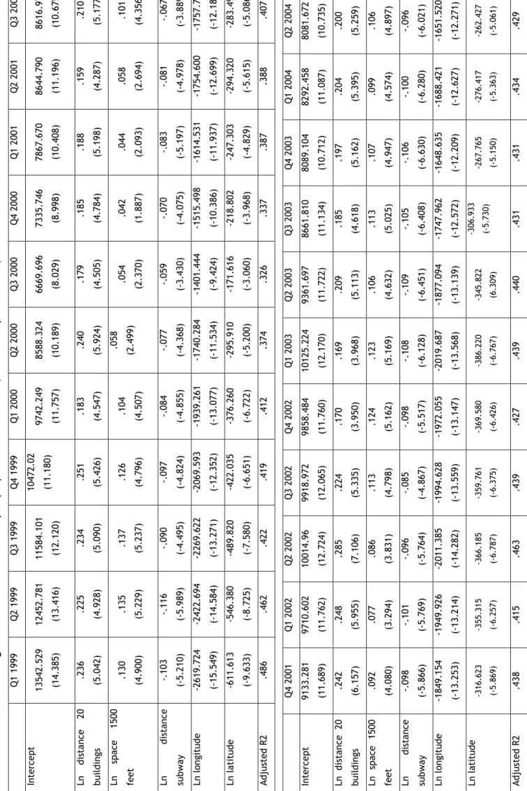
The results of the location-specific model (Model II) are reported in Table 3. The inverse of the weighted average distance of the 20 closest office buildings proves significant in this estimation as well as the number of square feet of office space located within 1500 feet. Distance to a subway station is also confirmed to be relevant in rental rate determination. Finally, latitude and longitude coordinates, proxying spatial effects not operationalized in the other variables of the model are also significant in the hedonic regression. The negative coefficient of the latitude variable indicates that average rental rates decrease the further south a property is located in Manhattan. While this is a highly generalized finding, it is in line with observations that office rents are highest in the northern section of Midtown while buildings in Midtown South and Downtown command lower rents on average. Similarly, the longitude variable also has a negative sign which entails that buildings located in the western part of Manhattan have lower rents than those located in the eastern part. While office locations on the western sections of Midtown Manhattan have experienced positive dynamics in recent years, the overall prime office locations are still to be found in the largest office cluster around the Plaza District located in the northeastern section of Midtown Manhattan.

(25)

T a b le 2 : H ed o n ic r e g res si o n m o d el I : p ro p er ty -s p e ci fi c p ri ce d et er m in a n ts ( t-v a lu es i n p a ren th es es ) Q 1 2 0 0 2 Q 2 2 0 0 2 Q 3 2 0 0 2 Q 4 2 0 0 2 Q 1 2 0 0 3 Q 2 2 0 0 3 Q 3 2 0 0 3 Q 4 2 0 0 3 Q 1 2 0 0 4 Q 2 2 0 0 4 In te rc e p t -6 9 .9 9 9 (-8 .4 1 6 ) -6 4 .8 9 9 (-8 .1 3 0 ) -6 5 .1 0 3 (-7 .6 4 8 ) -6 4 .9 5 6 (-7 .7 2 7 ) -7 3 .0 7 4 (-8 .8 1 9 ) -7 5 .4 4 3 (-9 .5 4 6 ) -7 6 .1 4 3 (-1 0 .1 7 8 ) -7 6 .1 4 3 (-1 0 .0 8 6 ) -7 4 .7 4 8 (-9 .5 8 5 ) -7 1 .2 2 9 (-9 .4 0 0 ) L n v a c a n c y -. 0 1 5 (-1 .3 8 7 ) -. 0 1 8 (-1 .6 8 5 ) -. 0 1 3 (-1 .2 7 1 ) -. 0 1 3 (-1 .1 0 6 ) -. 0 1 6 (-1 .4 0 4 ) -. 0 0 9 (-.8 2 5 ) -. 0 1 1 (-1 .0 1 0 ) -0 .0 1 1 (-1 .1 5 6 ) -0 .0 1 2 (-1 .3 6 7 ) -0 .0 1 5 (-.8 8 7 ) L n b u il d in g a re a .0 5 2 (2 .8 4 9 ) .0 6 0 (3 .3 8 9 ) .0 4 1 (2 .2 4 3 ) .0 4 2 (2 .3 0 4 ) .0 4 2 (2 .3 4 2 ) .0 3 8 (2 .1 6 4 ) .0 3 8 (2 .3 1 7 ) 0 .0 3 8 (2 .2 4 8 ) 0 .0 3 7 (1 .9 3 5 ) 0 .0 3 2 (1 .7 3 2 ) L n y e a r b u il t 9 .5 7 0 (8 .6 3 2 ) 8 .8 7 6 (8 .3 4 3 ) 8 .9 1 7 (7 .8 6 0 ) 8 .9 0 2 (7 .9 4 7 ) 9 .9 7 4 (9 .0 3 3 ) 1 0 .2 8 7 (9 .7 6 5 ) 1 0 .3 8 4 (1 0 .4 1 5 ) 1 0 .3 8 4 (1 0 .3 2 7 ) 1 0 .2 0 2 (9 .8 3 3 ) 9 .7 4 2 (9 .6 5 2 ) L n s to ri e s .1 6 3 (5 .0 2 0 ) .1 7 9 (5 .7 0 7 ) .2 1 5 (6 .3 6 6 ) .1 7 7 (5 .3 3 7 ) .1 7 4 (5 .3 1 9 ) .1 7 4 (5 .5 2 2 ) .1 5 5 (5 .1 7 6 ) 0 .1 5 5 (5 .0 3 2 ) 0 .1 4 9 (5 .5 3 2 ) 0 .1 6 4 (5 .6 4 9 ) L n a m e n it ie s .0 7 4 (1 .9 2 7 ) .0 7 8 (2 .1 3 6 ) .0 6 0 (1 .5 8 0 ) .0 9 2 (2 .3 7 8 ) .0 8 8 (2 .3 2 2 ) .0 9 8 (2 .6 2 4 ) .1 1 5 (3 .1 9 9 ) 0 .1 1 5 (3 .5 3 2 ) 0 .1 2 7 (3 .2 3 5 ) 0 .1 1 7 (3 .6 0 6 ) A d ju st e d R 2 .3 7 1 .4 0 5 .4 0 1 .3 6 2 .3 9 2 .3 9 6 .4 0 8 .4 0 8 .3 9 6 .3 9 3 Q 1 1 9 9 9 Q 2 1 9 9 9 Q 3 1 9 9 9 Q 4 1 9 9 9 Q 1 2 0 0 0 Q 2 2 0 0 0 Q 3 2 0 0 0 Q 4 2 0 0 0 Q 1 2 0 0 1 Q 2 2 0 0 1 Q 3 2 0 0 1 Q 4 2 0 0 1 In te rc e p t -7 5 .4 6 6 (-6 .6 4 7 ) -8 3 .2 0 7 (-8 .0 5 3 ) -7 7 .8 2 0 (-7 .8 4 8 ) -7 0 .7 6 2 (-7 .3 7 6 ) -6 2 .0 7 7 (-7 .6 5 8 ) -6 2 .4 9 2 (-7 .2 7 5 ) -5 7 .7 2 5 (-6 .4 1 2 ) -5 3 .8 1 7 (-5 .7 6 1 ) -5 6 .0 5 5 (-6 .3 0 8 ) -5 2 .4 2 2 (-5 .6 9 9 ) -6 9 .8 2 0 (-7 .0 4 6 ) -6 4 .7 6 3 (-7 .8 1 6 ) L n v a c a n c y -. 0 2 5 (-1 .5 7 9 ) -. 0 2 4 (-1 .6 0 0 ) -. 0 2 7 (-1 .8 7 8 ) -. 0 2 7 (-1 .9 5 8 ) -. 0 2 1 (-1 .8 5 9 ) -. 0 1 5 (-1 .2 5 9 ) -. 0 0 8 (-.6 8 1 ) -. 0 1 8 (1 .4 2 8 ) -. 0 0 3 (. 2 4 1 ) -. 0 1 2 (. 9 0 0 ) -. 0 1 3 (. 9 6 5 ) -. 0 2 1 (-1 .8 7 8 ) L n b u il d in g a re a .0 6 5 (2 .5 3 8 ) .0 5 1 (2 .1 4 2 ) .0 5 4 (2 .3 0 7 ) .0 8 2 (3 .6 4 3 ) .0 7 6 (3 .9 1 9 ) .0 3 5 (1 .7 5 5 ) .0 3 9 (1 .8 5 1 ) .0 4 2 (1 .9 3 0 ) .0 4 8 (2 .4 4 6 ) .0 5 4 (2 .6 5 5 ) .0 3 2 (1 .4 7 4 ) .0 6 0 (3 .2 9 4 ) L n y e a r b u il t 1 0 .2 3 1 (6 .7 7 2 ) 1 1 .3 0 2 (8 .2 2 2 ) 1 0 .5 9 3 (8 .0 2 9 ) 9 .6 4 4 (7 .5 5 3 ) 8 .4 9 8 (7 .8 6 9 ) 8 .6 1 8 (7 .5 3 8 ) 7 .9 8 6 (6 .6 6 9 ) 7 .4 6 4 (6 .0 0 7 ) 7 .7 7 5 (6 .5 7 5 ) 7 .2 7 6 (5 .9 4 6 ) 9 .5 8 7 (7 .2 7 2 ) 8 .8 7 6 (8 .0 3 7 ) L n s to ri e s .1 8 4 (3 .4 5 4 ) .1 4 0 (2 .9 4 1 ) .1 3 3 (2 .9 0 2 ) .1 0 4 (2 .3 3 3 ) .1 1 4 (3 .1 5 5 ) .1 4 4 (3 .8 7 6 ) .1 7 6 (4 .4 4 1 ) .1 9 6 (4 .7 4 6 ) .1 2 9 (3 .3 8 3 ) .1 5 0 (3 .7 8 5 ) .1 8 2 (4 .3 9 4 ) .1 5 9 (4 .9 2 0 ) L n a m e n it ie s .0 6 3 (1 .1 8 0 ) .0 5 1 (1 .0 2 1 ) .0 6 4 (1 .3 2 8 ) -. 0 1 7 (-.3 6 3 ) .0 5 0 (1 .1 6 5 ) .0 4 9 (1 .1 9 4 ) -. 0 1 1 (-1 .2 7 7 ) -. 0 1 1 (-.2 5 4 ) -. 0 1 7 (-.4 3 7 ) -. 0 2 7 (-.6 4 3 ) .0 3 2 (. 7 5 3 ) .0 6 7 (1 .7 8 3 ) A d ju st e d R 2 .3 7 5 .3 6 5 .3 6 4 .3 6 1 .3 6 1 .2 9 7 .3 0 4 .2 9 7 .2 8 4 .2 8 5 .3 3 3 .3 7 2

(26)

T a b le 3 : H ed o n ic r e g res si o n m o d el I I: l o ca ti o n -s p e ci fi c p ri ce d et er m in a n ts ( t-v a lu es i n p a ren th es es ) Q 1 1 9 9 9 Q 2 1 9 9 9 Q 3 1 9 9 9 Q 4 1 9 9 9 Q 1 2 0 0 0 Q 2 2 0 0 0 Q 3 2 0 0 0 Q 4 2 0 0 0 Q 1 2 0 0 1 Q 2 2 0 0 1 Q 3 2 0 0 1 In te rc e p t 1 3 5 4 2 .5 2 9 (1 4 .3 8 5 ) 1 2 4 5 2 .7 8 1 (1 3 .4 1 6 ) 1 1 5 8 4 .1 0 1 (1 2 .1 2 0 ) 1 0 4 7 2 .0 2 (1 1 .1 8 0 ) 9 7 4 2 .2 4 9 (1 1 .7 5 7 ) 8 5 8 8 .3 2 4 (1 0 .1 8 9 ) 6 6 6 9 .6 9 6 (8 .0 2 9 ) 7 3 3 5 .7 4 6 (8 .9 9 8 ) 7 8 6 7 .6 7 0 (1 0 .4 0 8 ) 8 6 4 4 .7 9 0 (1 1 .1 9 6 ) 8 6 1 6 .9 7 6 (1 0 .6 7 5 ) L n d is ta n c e 2 0 b u il d in g s .2 3 6 (5 .0 4 2 ) .2 2 5 (4 .9 2 8 ) .2 3 4 (5 .0 9 0 ) .2 5 1 (5 .4 2 6 ) .1 8 3 (4 .5 4 7 ) .2 4 0 (5 .9 2 4 ) .1 7 9 (4 .5 0 5 ) .1 8 5 (4 .7 8 4 ) .1 8 8 (5 .1 9 8 ) .1 5 9 (4 .2 8 7 ) .2 1 0 (5 .1 7 7 ) L n sp a c e 1 5 0 0 fe e t .1 3 0 (4 .9 0 0 ) .1 3 5 (5 .2 2 9 ) .1 3 7 (5 .2 3 7 ) .1 2 6 (4 .7 9 6 ) .1 0 4 (4 .5 0 7 ) .0 5 8 (2 .4 9 9 ) .0 5 4 (2 .3 7 0 ) .0 4 2 (1 .8 8 7 ) .0 4 4 (2 .0 9 3 ) .0 5 8 (2 .6 9 4 ) .1 0 1 (4 .3 5 6 ) L n d is ta n c e su b w a y -. 1 0 3 (-5 .2 1 0 ) -. 1 1 6 (-5 .9 8 9 ) -. 0 9 0 (-4 .4 9 5 ) -. 0 9 7 (-4 .8 2 4 ) -. 0 8 4 (-4 .8 5 5 ) -. 0 7 7 (-4 .3 6 8 ) -. 0 5 9 (-3 .4 3 0 ) -. 0 7 0 (-4 .0 7 5 ) -. 0 8 3 (-5 .1 9 7 ) -. 0 8 1 (-4 .9 7 8 ) -. 0 6 7 (-3 .8 8 9 ) L n l o n g it u d e -2 6 1 9 .7 2 4 (-1 5 .5 4 9 ) -2 4 2 2 .6 9 4 (-1 4 .5 8 4 ) -2 2 6 9 .6 2 2 (-1 3 .2 7 1 ) -2 0 6 9 .5 9 3 (-1 2 .3 5 2 ) -1 9 3 9 .2 6 1 (-1 3 .0 7 7 ) -1 7 4 0 .2 8 4 (-1 1 .5 3 4 ) -1 4 0 1 .4 4 4 (-9 .4 2 4 ) -1 5 1 5 .4 9 8 (-1 0 .3 8 6 ) -1 6 1 4 .5 3 1 (-1 1 .9 3 7 ) -1 7 5 4 .6 0 0 (-1 2 .6 9 9 ) -1 7 5 7 .7 3 6 (-1 2 .1 8 6 ) L n l a ti tu d e -6 1 1 .6 1 3 (-9 .6 3 3 ) -5 4 6 .3 8 0 (-8 .7 2 5 ) -4 8 9 .8 2 0 (-7 .5 8 0 ) -4 2 2 .0 3 5 (-6 .6 5 1 ) -3 7 6 .2 6 0 (-6 .7 2 2 ) -2 9 5 .9 1 0 (-5 .2 0 0 ) -1 7 1 .6 1 6 (-3 .0 6 0 ) -2 1 8 .8 0 2 (-3 .9 6 8 ) -2 4 7 .3 0 3 (-4 .8 2 9 ) -2 9 4 .3 2 0 (-5 .6 1 5 ) -2 8 3 .4 9 5 (-5 .0 8 6 ) A d ju st e d R 2 .4 8 6 .4 6 2 .4 2 2 .4 1 9 .4 1 2 .3 7 4 .3 2 6 .3 3 7 .3 8 7 .3 8 8 .4 0 7 Q 4 2 0 0 1 Q 1 2 0 0 2 Q 2 2 0 0 2 Q 3 2 0 0 2 Q 4 2 0 0 2 Q 1 2 0 0 3 Q 2 2 0 0 3 Q 3 2 0 0 3 Q 4 2 0 0 3 Q 1 2 0 0 4 Q 2 2 0 0 4 In te rc e p t 9 1 3 3 .2 8 1 (1 1 .6 8 9 ) 9 7 1 0 .6 0 2 (1 1 .7 6 2 ) 1 0 0 1 4 .9 6 (1 2 .7 2 4 ) 9 9 1 8 .9 7 2 (1 2 .0 6 5 ) 9 8 5 8 .4 8 4 (1 1 .7 6 0 ) 1 0 1 2 5 .2 2 4 (1 2 .1 7 0 ) 9 3 6 1 .6 9 7 (1 1 .7 2 2 ) 8 6 6 1 .8 1 0 (1 1 .1 3 4 ) 8 0 8 9 .1 0 4 (1 0 .7 1 2 ) 8 2 9 2 .4 5 8 (1 1 .0 8 7 ) 8 0 8 1 .6 7 2 (1 0 .7 3 5 ) L n d is ta n c e 2 0 b u il d in g s .2 4 2 (6 .1 5 7 ) .2 4 8 (5 .9 5 5 ) .2 8 5 (7 .1 0 6 ) .2 2 4 (5 .3 3 5 ) .1 7 0 (3 .9 5 0 ) .1 6 9 (3 .9 6 8 ) .2 0 9 (5 .1 1 3 ) .1 8 5 (4 .6 1 8 ) .1 9 7 (5 .1 6 2 ) .2 0 4 (5 .3 9 5 ) .2 0 0 (5 .2 5 9 ) L n sp a c e 1 5 0 0 fe e t .0 9 2 (4 .0 8 0 ) .0 7 7 (3 .2 9 4 ) .0 8 6 (3 .8 3 1 ) .1 1 3 (4 .7 9 8 ) .1 2 4 (5 .1 6 2 ) .1 2 3 (5 .1 6 9 ) .1 0 6 (4 .6 3 2 ) .1 1 3 (5 .0 2 5 ) .1 0 7 (4 .9 4 7 ) .0 9 9 (4 .5 7 4 ) .1 0 6 (4 .8 9 7 ) L n d is ta n c e su b w a y -. 0 9 8 (-5 .8 6 6 ) -. 1 0 1 (-5 .7 6 9 ) -. 0 9 6 (-5 .7 6 4 ) -. 0 8 5 (-4 .8 6 7 ) -. 0 9 8 (-5 .5 1 7 ) -. 1 0 8 (-6 .1 2 8 ) -. 1 0 9 (-6 .4 5 1 ) -. 1 0 5 (-6 .4 0 8 ) -. 1 0 6 (-6 .6 3 0 ) -. 1 0 0 (-6 .2 8 0 ) -. 0 9 6 (-6 .0 2 1 ) L n l o n g it u d e -1 8 4 9 .1 5 4 (-1 3 .2 5 3 ) -1 9 4 9 .9 2 6 (-1 3 .2 1 4 ) -2 0 1 1 .3 8 5 (-1 4 .2 8 2 ) -1 9 9 4 .6 2 8 (-1 3 .5 5 9 ) -1 9 7 2 .0 5 5 (-1 3 .1 4 7 ) -2 0 1 9 .6 8 7 (-1 3 .5 6 8 ) -1 8 7 7 .0 9 4 (-1 3 .1 3 9 ) -1 7 4 7 .9 6 2 (-1 2 .5 7 2 ) -1 6 4 8 .6 3 5 (-1 2 .2 0 9 ) -1 6 8 8 .4 2 1 (-1 2 .6 2 7 ) -1 6 5 1 .5 2 0 (-1 2 .2 7 1 ) L n l a ti tu d e -3 1 6 .6 2 3 (-5 .8 6 9 ) -3 5 5 .3 1 5 (-6 .2 5 7 ) -3 6 6 .1 8 5 (-6 .7 8 7 ) -3 5 9 .7 6 1 (-6 .3 7 5 ) -3 6 9 .5 8 0 (-6 .4 2 6 ) -3 8 6 .2 2 0 (-6 .7 6 7 ) -3 4 5 .8 2 2 (6 .3 0 9 ) -3 0 6 .9 3 3 (-5 .7 3 0 ) -2 6 7 .7 6 5 (-5 .1 5 0 ) -2 7 6 .4 1 7 (-5 .3 6 3 ) -2 6 2 .4 2 7 (-5 .0 6 1 ) A d ju st e d R 2 .4 3 8 .4 1 5 .4 6 3 .4 3 9 .4 2 7 .4 3 9 .4 4 0 .4 3 1 .4 3 1 .4 3 4 .4 2 9

(27)

Hedonic analysis and spatiotemporal stability of rent determinants

Parameter estimates and phases of the market cycle

The explanatory power of the quarterly estimations varies considerably with R squares of the hedonic models ranging from 0.284 in the first quarter of 2001 to 0.408 in the third quarter of 2001 for Model I and 0.486 in the first quarter of 1999 to 0.326 in the third quarter of 2000 for Model II. Among individual parameter estimates, it is noteworthy that the parameter value of the amenities variable appears to be low in times of increasing rents and increases during the subsequent recession, which may indicate that the predictive power of these distinctive quality features for the average rent level of a building diminishes during a general shortage of space in the peak phase of the real estate cycle.

In the next step, the two hedonic models outlined above were pooled for each of the phases of the market cycle as defined in the methodology section. The results are reported in Table 4. There are considerable differences in parameter estimates between the peak phase on the one hand and the recovery and decline phases on the other as evidenced by the Chow tests for the entire model and the Tiao-Goldberger F tests for individual parameters. The Chow tests reject the null hypothesis of equal parameters in all three phases for all variables in both models.

Individual FTG values show that parameter values are significantly different in each phase of the

market cycle.

The results appear counter-intuitive at first sight. All variables with the exception of the number of stories have higher coefficients during the recovery and decline phase than they do during the peak phase. A possible explanation for this phenomenon is that the price convergence during the peak phase lowers the explanatory value of most quality features of buildings. During the peak phase of the market, Class A buildings are typically fully rented and demand for office space spills over to Class B buildings. As a consequence, the rent gap between Class A and Class B buildings narrows. Figure 5 illustrates the convergence dynamics of the three categories. I will explore this potential 'spillover effect' in more detail in the next section.

(28)

27

Figure 5: Quarterly growth rates of office rents by A/B/C quality class

Table 4: Hedonic regression (Model I and II) at various phases in the market cycle (longitudinal)

Model I

recovery peak decline pooled FTG

Intercept -69.577 (-19.974) -43.771 (-10.033) -65.781 (-29.584) -63.376 (-35.708) 12.39* Ln vacancy -.003 (-1.142) .012 (4.114) -.005 (-2.715) -.005 (-3.840) 8.24* Ln building area .072 (8.881) .038 (3.853) .041 (8.410) .051 (12.757) 4.109* Ln year built 9.466 (20.395) 6.132 (10.559) 9.005 (30.382) 8.676 (36.685) 4.218* Ln stories .121 (8.113) .145 (7.866) .172 (19.523) .159 (21.893) 3.956* Ln amenities .130 (8.008) .147 (7.406) .157 (15.583) .148 (18.261) 3.699* Adjusted R2 .344 .289 .373 .345 Chow Test 17.483*

(29)

28

Model II

recovery peak decline pooled FTG

Intercept 9447.545 (29.516) 6709.689 (17.436) 7763.999 (40.165) 7997.713 (50.637) 12.87* Ln distance 20 buildings .064 (15.472) .057 (11.283) .061 (21.948) .062 (28.663) 7.353* Ln space 1500 feet .170 (17.520) .117 (9.804) .164 (27.944) .159 (33.173) 3.955* Ln distance subway -.103 (-15.127) -.087 (-10.607) -.105 (-24.737) -.101 (-29.406) 8.022* Ln longitude -1863.439 (-32.276) -1370.784 (-19.761) -1558.919 (-44.859) -1601.620 (-56.321) 8.191* Ln latitude -384.823 (-18.042) -217.973 (-8.427) -284.172 (-21.505) -297.632 (-27.848) 8.119* Adjusted R2 .405 .360 .423 .392 Chow Test 27.494*

* significant at the 5% level

Cross-sectional parameter stability and market fragmentation

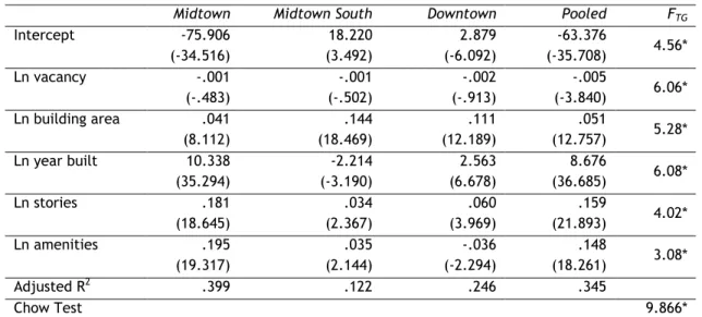
To test the hypothesis of parameter stability across submarkets, both hedonic models are parametrized separately for each of the three aggregated submarkets (Midtown, Midtown South and Downtown Manhattan) and subsequently compared to the pooled model. Table 5 shows the parameter estimates for both models. Among the three submarkets tested, the model performs best for Midtown and Downtown Manhattan but barely reaches the required significance levels for Midtown South. The t values of individual coefficients indicate that some variables that are positive and significant in the other two submarkets do not necessarily show the expected contribution to rental rates in a third market. Moreover, building age has a negative signs in the Midtown South market. This might be attributable to specifics of the Midtown South submarket inventory. A large proportion of the buildings in this market are either historic buildings with landmark status (Madison Square, Gramercy Park) or former warehouse buildings converted for office use, particularly for the information technology industry. Consequently, older buildings generally command higher rents in this submarket than more recently constructed buildings.

(30)

29

With regard to the submarket estimates of location-specific variables (Model II), Midtown Manhattan exhibits significantly better explanatory power than the other two submarkets (Table 5). This is particularly evident in the Downtown market where the spatial variables barely reach the desired significance levels. Geographical characteristics of the Downtown area may explain this phenomenon. First, due to the narrowness of the land area between the Hudson and East Rivers there is no distinct differentiation of the submarket into a western and an eastern section as is the case in Midtown Manhattan. Second, because of the narrowness of the geographic shape of the area and the resulting high density of the subway system in the Downtown area, accessibility by subway and proximity to other office buildings are of lesser predictive value for rental rates than in Midtown South which exhibits a more even grid-like pattern with both core and peripheral locations and longer average distances between subway stations. While easy access to rapid transit is almost ubiquitous in the Downtown area, this is not necessarily the case in the Midtown Manhattan.

Again, the Chow test confirms that the estimated parameters are significantly different from

one another in the three submarket areas. The individual FTG values show that parameters

differ significantly both across subareas with two notable exceptions (the amount of space within 1500 feet and the distance to the nearest subway station). Since the parameters of these variables are not significantly different, one may conclude that these variables are valued similarly in all submarkets in determining the rental rate of a given building. For all other parameters, significant differences were found.

(31)

30

Table 5: Hedonic regression (Model I and II) for subareas (cross-sectional)

Model I

Midtown Midtown South Downtown Pooled FTG

Intercept -75.906 (-34.516) 18.220 (3.492) 2.879 (-6.092) -63.376 (-35.708) 4.56* Ln vacancy -.001 (-.483) -.001 (-.502) -.002 (-.913) -.005 (-3.840) 6.06* Ln building area .041 (8.112) .144 (18.469) .111 (12.189) .051 (12.757) 5.28* Ln year built 10.338 (35.294) -2.214 (-3.190) 2.563 (6.678) 8.676 (36.685) 6.08* Ln stories .181 (18.645) .034 (2.367) .060 (3.969) .159 (21.893) 4.02* Ln amenities .195 (19.317) .035 (2.144) -.036 (-2.294) .148 (18.261) 3.08* Adjusted R2 .399 .122 .246 .345 Chow Test 9.866* Model II

Midtown Midtown South Downtown Pooled FTG

Intercept 6934.917 (39.304) 4625.633 (12.583) -5764.091 (-6.805) 7997.713 (50.637) 8.87* Ln distance 20 buildings .060 (18.758) .039 (10.454) .057 (11.384) .062 (28.663) 9.69* Ln space 1500 feet .134 (21.049) .038 (2.451) .050 (5.043) .159 (33.173) 1.41 Ln distance subway -.091 (-22.179) -.010 (-1.288) .006 (.659) -.101 (-29.406) 1.26 Ln longitude -1962.017 (-64.949) -562.577 (-8.506) 994.468 (6.430) -1601.620 (-56.321) 9.95* Ln latitude 407.473 (17.593) -593.907 (-18.413) 400.899 (7.952) -297.632 (-27.848) 9.59* Adjusted R2 .513 .114 .102 .392 Chow Test 13.589*

* significant at the 5% level

Rental rate convergence of Class A/B/C properties and the market cycle

As reported above, a convergence effect of rental rates of the three quality classes of office buildings (A,B,C) is observed around the peak of the market cycle. Figure 6 illustrates how rental rates of Class B buildings approach Class A rents during the peak phase of the market. Thus, distinctive quality features of buildings as represented by the variables of the two hedonic regressions lose some of their explanatory power as rental rates converge. As soon as

(32)

31

the decline phase begins, rental rates start to diverge again, as tenants have a larger variety of available office buildings to choose from in times of higher vacancy rates. Therefore, the quality features of buildings regain their relative importance and predictive power as the spread of rental rates increases. To corroborate these results, I apply a one-way ANOVA test for equal means of rental rates to office buildings of the three quality categories A, B, C (Table 6). While the mean rental rates differ significantly for these three groups throughout the analyzed period (all values are significant at the 1% level), the F test values as well as the robust Welch and Brown-Forsythe values are lower at the peak of the cycle (Q3-2000 through Q1-2001), indicating that the mean rental rates of the three categories become more similar at the peak of the market cycle. Interestingly, as differences of mean rental rates decrease between groups, within-group variation increases and vice versa. This may indicate that the reported convergence of rental rates affects only a selective group of Class B and C properties with competitive features, while the rest of buildings in these categories remain largely unaffected by the upswing of the market. Further research is needed, however, to confirm these results.

Figure 6: Convergence of rental rates during the peak phase of the market cycle: average rental rates (above) and rental rates in Class B buildings as a percentage of Class A rental rates. Data: CoStar Group, Grubb & Ellis.

(33)

32 Panel estimation

In the next step of the empirical investigation, I estimate random-effects GLS models to simultaneously capture cross-sectional and time-series effects.

Table 6 shows the results of the location-specific model containing all 16,857

observations. The significance of the variables a) distance to subway, b) 20 closest buildings as well as the c) square footage within a 1500 feet radius are confirmed. The R square measures reveal that within effects equal zero since the explanatory variables used in this specification remain fixed throughout the observed period. The GLS random-effects model is then estimated for the property-specific factors (Table 7). Again, the results confirm that rentable building area, age, height and amenities are significant and show the expected signs.

In the next step, I modify the model so that both location- and property-specific variables are included along with the time-varying variables. Not surprisingly, pooling the variables of Model I and Model II into a single model yields a larger joint explanation of variance (Table 8). At the same time, the number of valid observations decreases sharply from over 15,000 in the separate models to below 5,000 in the pooled model. This is due to the fact that only one third of all buildings have complete and valid entries in all variable columns. Thus, the selected sample that fulfills the requirement of complete information is much smaller. Because multicollinearity is a more serious concern in the pooled model than it is in the separate models, all variables inducing significant multicollinearity are removed automatically.

This pooled model is then used to estimate separate regressions for each of the three quality classes (A/B/C). The results illustrate that the hedonic model exhibits the highest explanatory power for Class A properties (Table 9) while the model is less significant in the Class B (Table 10) and Class C (Table 11). This observation is in line with the

expectation of a more competitive pricing scheme in the upper segments of the market. A closer inspection of individual coefficients yields that many of the variables in the

specified random-effects model fail to be significant. One possible explanation for this is that the prevalence of time-invariant hedonic features in the model reduces the overall goodness of fit in a panel data model compared to the initially estimated cross-sectional OLS model where no such effect is measured.

(34)

33

When estimating the pooled model separately for the three subareas, the highest explanatory power is found for the Midtown South area and the lowest for the Downtown area with Midtown Manhattan taking an intermediate position (Tables 12 through 14). Among individual variables, the distance to the 20 closest buildings does not show up significant in any of the estimates. It is noteworthy that the time-varying variables sublet rate (significant at 10%) and vacancy rate (significant at 1%) fail to generate a within-effect of a sufficiently large order of magnitude (R square of 0.0034). There are several possible explanations for this. First, the weight of the time-invariant variables diminishes the within effects so that the effect of the two time-varying variables is underestimated. Second, while vacancy rates contribute to explaining differences in rental rates between buildings, the dynamic relationship of vacancy and rental rates within a building over time is not easily captured by this model. Although all submarket estimations are jointly significant, the values of the coefficients and their individual significance levels vary to a great degree. R square values range from 0.13 in Gramercy Park to 0.60 in the World

Trade Center submarket. The R square of within effects is largely a function of the

significance of the vacancy rate variable in the model, the only time-varying variable in this specification. Direct comparisons of variable coefficients in submarkets are encumbered by large differences in sample size, however. Nevertheless, these findings corroborate the results regarding non-homogenous parameters across spatial units obtained earlier in Chow tests of the OLS models.

Finally, Table 15 reports the Arellano-Bond dynamic panel-data estimation. As outlined above, the exogenous variables are used as instrumental variables in the two-step estimation process. The included dynamic variables (lagged rent, sublet vacancy rate and

overall vacancy rate) are significant with a p-value below 5%. While the lagged value rit-1

explains the largest part of the panel dynamics, the lagged vacancy measures exhibit the expected negative impact on subsequent changes in rental rates.

These results have to be interpreted with caution, however, since the value of the Sargan test for over-identifying restrictions indicates problems with the correct model specification in this case. More importantly, however, the Arellano-Bond tests for autocovariance in residuals of order 2 fail to reject the null hypothesis of no autocorrelation, which speaks in favor of the selected model specification.

(35)

34

Table 6: Pooled model, all observations location-specific model

Random-effects GLS regression Number of obs = 16857

Number of groups = 999

R-sq: within = 0.0000 Obs per group: min = 1

between = 0.3302 avg = 16.9

overall = 0.2770 max = 22

Random effects u_i ~ Gaussian Wald chi2(4) = 491.79

corr(u_i, X) = 0 (assumed) Prob > chi2 = 0.0000

ln_rent Coef. Std. Err. z P>z [95% Conf. Interval]

ln_latitude 206.5662 20.77073 9.95 0.000 165.8564 247.2761 ln_subway -.0910125 .0131596 -6.92 0.000 -.1168048 -.0652202 ln_distance_20 bldgs .0640123 .0077423 8.27 0.000 .0488376 .079187 ln_sq.ft within1500 ft .2196119 .0183301 11.98 0.000 .1836856 .2555382 _cons -765.7518 76.99502 -9.95 0.000 -916.6592 -614.8443 sigma_u .275489 sigma_e .18886561

rho .6802724 (fraction of variance due to u_i)

Table 7: Pooled model, all observations building-specific model

between = 0.3567 avg = 16.4

ln_building area .0507835 .0138267 3.67 0.000 .0236837 .0778833 ln_year built 7.406912 .8038323 9.21 0.000 5.831429 8.982394 ln_stories .1215857 .023873 5.09 0.000 .0747954 .168376 ln_amenities .159432 .027396 5.82 0.000 .1057367 .2131272 _cons -53.66099 6.028466 -8.90 0.000 -65.47656 -41.84541 sigma_u .27087204 sigma_e .18898711

(36)

35

Table 8: Variables of Model I and Model II combined into a single model

between = 0.5001 avg = 6.8

ln_latitude 228.0741 21.62577 10.55 0.000 185.6883 270.4598 ln_subway distance -.0501038 .0143679 -3.49 0.000 -.0782644 -.0219433 ln_distance 20 bldgs .0001392 .0119052 0.01 0.991 -.0231946 .0234731 ln_sq.ft within1500 ft .1087543 .0197927 5.49 0.000 .0699614 .1475473 ln_rba .0377657 .0156743 2.41 0.016 .0070446 .0684868 ln_year built 6.29816 .9242095 6.81 0.000 4.486742 8.109577 ln_stories .1300208 .0336101 3.87 0.000 .0641461 .1958954 ln_amenities .1032081 .0304887 3.39 0.001 .0434513 .1629649 ln_sublet .006864 .003874 1.77 0.076 -.0007289 .0144568 ln_vacancy -.0132697 .0050022 -2.65 0.008 -.0230737 -.0034656 _cons -892.0535 79.61368 -11.20 0.000 -1048.093 -736.0136 sigma_u .22661135 sigma_e .14696903