Credit contagion

(1)

CREDIT

CONTAGION

by

Arnhild Kløvnes

MASTER THESIS

for the degree

Master of Science in Modeling and Data Analysis

Faculty of Mathematics and Natural Sciences

The University of Oslo

(2)

(3)

Acknowledgements

I have spent half a year on this thesis, and it has been a very interesting and in-structive period. I have gained useful knowledge that I will bring with me further in life. I wish to thank my supervisor, Giulia Di Nunno, for giving me this inter-esting topic to study. I am grateful for her taking the time to patiently push me in the right direction and for being so precise. I would like to thank my family for being so understanding, patient and encouraging. I would also like to thank Asma Khedher for helping me getting started with the tools needed for my presentation.

(4)

Preface

The aim of my study has been to review models for credit contagion finalizing the study to the computation of derivative prices. Credit contagion is a fairly new field to be studied. Kusuoka introduced a way to model dependent defaults in 1998 and Davis and Lo, [4], introduced a model for default contagion in 2001. Credit contagion is an element of credit risk. Credit risk consists of individual risk ele-ments, such as default probability and recovery rates, and it consists of portfolio risk elements like default correlation. There are roughly two approaches to model credit risk; structural modeling and intensity based modeling. The structural mod-els (also called firm value modmod-els) goes back to Merton. In these modmod-els, default is triggered when the value process (which might be modeled by a standard geometric Brownian motion) of a firm falls below a pre-determined default boundary. In the intensity based models (also known as reduced form models) default is typically described as a jump time of a jump process (for instance a Poisson process). Default is, as mentioned, an element of credit risk. Modeling credit risk is im-portaint when it comes to the modeling of derivative pricing, such as the prices of credit default swaps, (CDS), and collateral debt obligations, (CDO), which are basic protection contracts against default of firms in a portfolio. CDS’ and CDOs have been largely talked about during the latest financial crisis since, among oth-ers, credit rating agencies (which evaluate the default probability of issuers of debt securities) failed to adequately account for large risks when rating these products. Credit rating agencies, like Moody’s and Credit Suisse, calculate the default likeli-hood of firms. To model correlations between the default behavior of firms, Credit Suisse uses the correlations in equity values as a replacement for the correlations in the default probabilities (also known as correlations in credit quality). Moody’s uses the ’diversity score’ which is based on the binomial expansion technique, where independence between firms is assumed. Moody’s idea on how to capture correlations in a binomial distribution is to make a hypothetical portfolio consisting of less firms than the original one, and having the hypothetical firms being inde-pendent. Then a default in the ’new’ portfolio would correspond to, say, 2 defaults in the original portfolio. Other ways to model default and credit contagion might be to introduce primary and secondary firms, as in the approach of Jarrow and Yu, referred to in [6]. In the model by Jarrow and Yu the defaults of the primary firms are influenced by macoreconomic conditions (i.e. influenced by the gross domestic product, unemployment rate and inflation rate), but not by the credit risk of coun-terparties. The default of the secondary firm depends on the status of other firms, so it suffices to focus on securities issued by secondary firms. Kusuoka’s approach to model default dependence, which is also referred to in [6], is based on a change of probability measure. Kusuoka assumed that the default times were exponen-tially distributed. The probability measure is then changed so that the parameter of the exponential law belonging to one firm will jump to a pre-determined value as soon as the default of another firm occurs. Yet another approach is the one by

(5)

Davis and Lo, [4]. They model default in a portfolio by independent Bernoulli vari-ables where default can occur due to direct default of a company or by contagion. The model suggested by Biagini, Fuschini and Klüppelberg is based on the one by Davis and Lo.

My studies of the modeling of credit contagion and pricing of derivatives are based on the papers of Biagini, Fuschini and Klüppelberg [2] and of Hatchett and Kühn [3]. The paper is organized as follows: First I will give a short introduction to contagion and default, as well as a general calculation of derivative prices. In chapter 2 I will describe the default intensities for the discrete time model as in [3]. In chapter 3 the continuous time model will be described as in [2]. I will also compare some elements of the two models. The pricing of derivatives will be presented in the two chapters where the model description is taking place. Finally, I will present an extention of the continuous time contagion description in chapter 4. This extension consists in expanding the economic relationship between firms from not just being present or absent, but to try to say how much they can influence each other economically if they are in an economic relationship. This means that the extension is trying to describe which type of economic relationship the firms are in - a competitive or cooperative economic relationship.

(6)

(7)

Chapter 1

Introduction

Credit contagion arises when a company is in economic distress or if it defaults. The default of a company will have implications for any firm that is economically connected to this given company. The effect of the default, and thus the effect of the credit contagion, depends on which economic relation the defaulting company has with other firms. If they were in a cooperative relationship, the default would have a negative effect on the firms that are connected to the defaulting company. For instance, if a company goes bankrupt, it will have a negative effect on the credit situation of its service provider or on its bank connection. On the other hand, if they were in a competitive economic relation, the default would have a positive effect on the firms that are connected to the defaulting company. For example, if there is a default within a business section, the number of orders might increase for the surviving firms.

One of the main worries when investing in a portfolio consisting of defaultable bonds is to not recieve the promised payment at the date of maturity, and this may occur if a bond defaults. If one bond defaults, there might be the risk of default contagion resulting in several defaults within the portfolio. Hence, the loss will be even larger. This is one of the reasons why one is interested in credit contagion.

1.1

Intensity based default

Default in an intensity based model is specified in terms of a jump process, and the jump occurs at timeτ which is typically modeled as a jump time of a jump process. What drives contagion are the default intensities of the firms within the portfolio. The default probability is the probability that the obligor or counterparty will de-fault on its contractual obligations to repay its debt, [5]. Denote the random time of default byτ : Ω_→R+which is defined on a probability space(Ω,_F,P). τ is assumed to be unbounded and non-negative. LetF = (Ft)t≥0. Further, consider

the filtrationG= (_Gt)t_≥0, where, for anyt,Gtis some givenσ-algebra which

(10)

with_Ft⊂ Gt.

1.1.1 Definitions regarding default

Default in an intensity based model is regarded as a stopping time with respect to a given filtration, and one has to consider the two different cases of continuous or discrete time. Starting with the definition for a discrete time model.

Definition (Stopping time in discrete time) AnF-stopping time on(Ω,_F,P)is a random variableτ : Ω_→ N_{∪ { ∞}} such that_{ω _∈Ω :τ(ω) =n_} is in_Fnfor

allninN.

The definition of the default time for a continuous time model is as follows:

Definition (Stopping time in continuous time) AnF-stopping time on(Ω,_F,P)

is a random variableτ : Ω_→ [0,_∞]such that_{ω _∈Ω :τ(ω)_≤ t_} is in_Ftfor

alltin [0,T].

Let F be the cumulative distribution function ofτ, thenF(t) =P(τ _≤t)for ev-erytinR+ is the default probability, and 1−F(t) = P(τ > t) is the survival probability. IfP(τ ∈(0,∞))>0the stopping time is non-trivial. The following definition is from [6].

Definition (Hazard and intensity function) An increasing function

Γ :R+_→R+given by the formula

Γ(t) :=−ln(1−F(t))for all t in R+,

is called the hazard function of τ. If the cumulative distribution function F is absolutely continuous with respect to the Lebesgue measure - that is, whenF(t) =

Rt

0 f(u)du, for a Lebesgue integrable functionf :R+→R+, then

F(t) = 1−e−Γ(t)= 1−e−R0tγ(u)du,

whereγ(t) =f(t)(1₋F(t))−1_{. The function}_γ _{is called the intensity function (or}

the hazard rate) of the random timeτ.

By assuming thatF(t) < 1, the hazard functionΓt is well defined for any t in

R+since the functionf is positive and the cumulative distribution function also is positive, the intensity functionγ is non-negative.

In order to give some examples of the different types of default intensities, one has to define some processes. Remember that a counting process N is defined through an increasing sequence _{T0, T1, . . .} of random variables, or random times, in

(11)

[0,_∞]. The process N is called non-explosive iflimnTn= +∞almost surely.

Re-call as well that a random variable X with outcomes{0,1,2, . . .} is Poisson dis-tributed with parameterλin(0,_∞), writtenX _{∼ P}o(λ), if P(X =x) = λ_xx_!e−λ

where0! = 1. The following definitions are from [7].

Definition (Poisson Process) A Poisson process is aG-adapted non-explosive count-ing process N with deterministic intensity λ > 0 such that R₀tλsds is finite

dt-almost everywhere for allt, with the property that, for alltands > t, conditional onGt, the random variable(Ns−Nt)∼ Po(

Rs t λudu).

The filtration(_Gt)t_≥0has been fixed in advance for the purpose of the definitions.

Alternatively, fors > t, one can say, since the increment(Ns−Nt)is independent

of theσ-fieldσ(Nu :u≤t), thatP

(Ns−Nt) =k|Gt =P (Ns−Nt) =k = (λ(s₋t))k k! e−λ(s−t).

Definition (Doubly Stochastic Process) Let N be aG-adapted non-explosive count-ing process with intensityλ > 0. N is doubly stochastic, driven byF, ifλisF -predictable and if, for alltands > t, conditional on the filtrationGt∨ Fs,

(Ns −Nt) ∼ Po(

Rs

t λ(ω, u))du. A doubly stochastic process is also called a

Cox process.

The intuition behind a doubly stochastic counting process is thatFtcontains enough

information to uncover the default intensityλt, but not information to uncover the

jump times of the counting process.

1.1.2 Some examples of default intensities

This thesis is not considering structural modeling, but just to have it mentioned: In the basic Merton model of default,τ happens when the value of the firm at the time of maturity, T, falls below the face value of the bond. Thus, default is only possible at T. And in the model of Black and Cox, τ is modeled as a first pas-sage time in which default happens when the value process of the firm reaches the level of its debt for the first time. In these kinds of models default is economic motivated. In the intensity based models defaults happen when an intensity based process makes a jump. One can mention three types of default intensities: constant-, deterministic- and stochastic default intensities.

In the three following cases, let τ be exponentially distributed with intensity pa-rameterλandτ := inf_{t > 0 : Nt = 1}, whereNtis a Poisson process. This

means that the time of default can be seen as the time of the first jump ofNt.

In a model where the default intensity is constant, the default probability is

(12)

is constant for allt. A Poisson process with constant intensityλ > 0is called a time-homogeneous Poisson process.

If one has a deterministic default intensity, then Nt ∼ Po(R₀tλudu). The

de-fault probability would beP(τ _≤ t) = 1₋e−R0tλudu. The intensity function is

γ(t) = λ(t) and it varies with the timet. A Poisson process with deterministic intensityλ >0is called a time-inhomogeneous Poisson process.

When one has the case of stochastic default intensity, Nt is a doubly stochastic

process which is Poisson distributed with parameterR₀tλ(ω, u)du. The parameter of the exponential distribution is λ(ω, u), and τ is a G-stopping time. Both the intensity and the stopping time are stochastic, and this is why a Cox process is sometimes called a doubly stochastic Poisson process. The general probability of default would be, fort_≤s,

P(t < τ ≤s|Gt) =E(1−e− Rs

t λ(ω,u)du|G_t).

And fort= 0, the default probability becomes

P(τ _≤s) =E(1₋e−R0sλ(ω,u)du).

The expectations are underP. In these two cases the intensity function isγ(s) =

λ(ω, s). The two expressions can be evaluated by the same means as in calculating the price of a default free zero coupon bond (a contract paying one unit of currency at the time of maturity), by lettingλtbe the short term interest rate,rt, and solve

the stochastic differential equation by, for instance, the Vasicek or CIR models. As an illustration one can consider the short term interest rate to be the instantaneous spot rate and the bank account to grow at each time instanttat a rate ofrt. One

can look, for example, at the fundamental pricing formula, found in [12]:

The price of an attainable contingent claim with payoffHT at timeT > tis given

by

Vt=EQ(e−

RT

t rsdsH_T|F_t) _(1.1)

where the risk neutral measureQ_∼Pis assumed to exist. Before moving on with the calculations, one can recall the meaning of an attainable claim:

A contingent claim is an_FT-measurable random variable F inL2(Q). The

contin-gent claim F is attainable on the given market model if there exists an admissible portfolio Z such that the value process of the portfolio at time T isVZ

y (T) = F

wherey = VZ₍₀₎_{. The portfolio Z is admissible if it is self-financing and lower}

bounded,VZ

t ≥ −K, K > 0 for alltP-almost surely. By self-financing one means

thatdVtZ =Zt·dXtwhereXt(i)is the price of securityiat timet, and the value

(13)

Moving on with the calculations of equation ( 1.1), let the short ratertbe the the

intensity functionλtandHT = 1as the face value of the zero coupon bond. By

ap-plying the Vasicek model, the dynamics ofλtis given by the stochastic differential

equation

dλt=a(b−λt)dt+σdBt (1.2)

where a,b andσ are positive constants. (The CIR model is similar to the expres-sion in equation ( 1.2), but where the termσdBt = σ

√

λtdBt). Btis a standard

one-dimensional Brownian motion generating_Ft. Note thatFcoinsides with the

filtration generated byλt. By lettingXt =−(b−λt) one gets that ( 1.2) can be

written as

dXt=−aXtdt+σdBt

X0=λ0−b

which is an Ohrnstein-Uhlenbeck process, and it is an affine process which means that it is Markovian and that there exists an explicit expression for ( 1.1). The Ornstein-Uhlenbeck process is solved by applying Itô’s formula with integrating factoreat, so

d(Xteat) =aeatXtdt+eat(−aXt+σdBt)

and by integrating fromstotand dividing by the integrating factor one gets Xt=Xse−a(t−s)+e−at

Z t s

σeaudBu, s≤t.

By substitutingXt=−(b−λt), the answer to equation ( 1.2) is

λt=λse−a(t−s)+b(1−e−a(t−s)) +σ

Z t s

e−a(t−u)dBu. (1.3)

The processλtis Gaussian. By looking atE(λt|Fs) andV ar(λt|Fs), one finds

that λt∼ N λse−a(t−s)+b(1−e−a(t−s)),σ 2 2a(1−e−2 a(t₋s)₎_{. By looking at}

limt_→∞E(λt) =b, one can regardbas a long term average intensity.

The dynamics forλtis underP. In order to use the pricing formula given in

equa-tion ( 1.1), one has to find the dynamics for the intensityλtunder the measureQ.

By Girsanov Theorem (theorem 8.6.6 in [13]) one gets thatB˜t = Bt+

Rt

0 qds,

whereq is in Randq = a(b−λt)−α

σ . Notice that q depends on tthrough λt, but

Vasicek assumed that the instantaneous spot rate (which is nowλt) under the

mea-sure Pevolves as an Ornstein-Uhlenbeck process with constant coefficients. By the given choice ofq it is also assumed that the coefficients are constant underQ

(14)

dλt=a(b−λt)dt+σdBt underP

dλt=a(b−

σq

a )dt−aλtdt+σdB˜t underQ.

The last equality could be stated asαtdt+σdB˜t, but in this case let(b−σq_a) = ˜b.

ThenX˜t=λt−˜bimplies that

dX˜t=−aX˜tdt+σdB˜t. (1.4)

This is an Ornstein-Uhlenbeck process under the measureQas well, so it is Gaus-sian with continuous paths. ForHT = 1, the pricing formula given in equation

( 1.1) can be written as Vt=EQ e−RtTλsds|F_t =E_Qe−RtTX˜s+˜b ds|F_t =e−RtT˜b dsE_Q e−RtTX˜sds|F_t . (1.5)

Since the coefficients in the Ornstein-Uhlenbeck equation are time-independent, one can write

E_Qe−RtTX˜sds|F_t

=F(T −t,X˜t) (1.6)

whereFis the function defined byF(θ, x) =E_Q(e−R0θX˜sxds)_andX˜x

s is the unique

solution of equation ( 1.4) satisfyingX˜x

0 =x. In this casex=λ0−˜bandX˜sxwill

just be writtenX˜s. Recall that the Laplace transformation of a random variable,

foruinR, isE(euX_{) =} R

Re

ux_P

X(dx). The expectation is calculated by Laplace

transformation of a Gaussian random varibale:

E_Qe−R0θX˜sds =e −EQ( Rθ 0 X˜sds)+1₂V arQ( Rθ 0 X˜s)ds .

The expectation becomes, where the first equality is due to Fubini’s,

E_Q( Z θ 0 ˜ Xsds) = Z θ 0 E_Q(λs−˜b)ds = Z θ 0 E_Q(λ0e−a(s)+ ˜b(1−e−a(s)) +σ Z s 0 e−a(s−u)dBu−˜b)ds = (λ0−˜b a )(1−e −aθ₎_. _(1.7) To calculateV arQ( Rθ

0 X˜sds)one starts out with writing the variance as the

(15)

respectively, the covariance is defined asCov(X, Y) =E(X−µX)(Y −µY) . Then V arQ( Z θ 0 ˜ Xsds) = Z θ 0 Z θ 0 Cov( ˜Xt,X˜u)du dt = Z θ 0 Z θ 0 (1 {t>u} +1{t≤u} )Cov( ˜Xt,X˜u)du dt. (1.8)

Looking at the expression for the covariance without the integrals and puttingX˜t=

λt−˜band by using the expression given in equation ( 1.3) , fors= 0, one gets

Cov( ˜Xt,X˜u) = E_Q λ0e−at+ ˜b(1−e−at) +σ Z t 0 e−a(t−s)dBs−˜b−(λ0e−at+ ˜b(1−e−at)−˜b) × λ0e−au+˜b(1−e−au) +σ Z t 0 e−a(u−s)dBs−˜b−(λ0e−au+˜b(1−e−au)−˜b) =E_Q(σe−at Z t 0 easdBs)(σe−au Z u 0 easdBs) =σ2e−a(t−u) Z t_∧u 0 e2asds =σ2e−a(t−u)(e 2a(t_∧u)₋₁₎ 2a .

Inserting this answer into equation ( 1.8), one is left with calculating Z θ 0 Z θ 0 σ2e−a(t−u)(e 2a(t_∧u)₋₁₎ 2a dudt = σ 2 2a Z θ 0 Z u 0 e−at−au+2at−e−at−audtdu +σ 2 2a Z θ 0 Z t 0 e−at−au+2at₋e−at−aududt = σ 2_θ a2 − σ2 a3(1−e− aθ₎ − σ 2 2a3(1−e− aθ₎2_. _(1.9)

Finally, by putting together the expressions for the expectation in equation ( 1.7) and the variance in equation ( 1.9), and by using equation ( 1.6), one gets that the pricing formula in equation ( 1.5) becomes:

(16)

exp_{{ −}˜b(T₋t)₋(λ0−˜b a )(1−e− a(T₋t)₎_} ×exp_{ 1 2 _σ2₍_T₋_t₎ a2 − σ2 a3(1−e− a(T₋t)₎₋ σ2 2a3(1−e− a(T₋t)₎2_}

which is more frequently expressed as

P(t, T) =e−(T−t)R(T−t,λt)_, _(1.10)

which is the affine structure mentioned previously, and whereR(T₋t, λt)is given

by R(θ, λ) = (˜b− σ 2 2a2)− 1 aθ (˜b− σ 2 2a2 −λ)(1−e− aθ₎₋ σ2 4a2(1−e− aθ₎2_.

If the model forλtis under the measureP, historical data should be used to estimate

the drift and volatility. If the model is under the measure Q, the risk adjusted drift and volatility can only be inferred from existing prices. One drawback of the Vasicek model is ifb = λt, then the dynamics becomedλt = σdBt and one has

a random walk. The Brownian component can take positive and negative values, so the intensity λt might be negative, and default intensities are supposed to be

positive . In the CIR model the default intenstiy will not become negative, but the process is not Gaussian and explicit formulae are more difficult to come by.

(17)

Chapter 2

Contagion model in discrete time

The paper of Hatchett and Kühn, [3], describes credit contagion in a discrete time framework. They are using probability theory to express their findings. The results are based on the use of the Law of Large Numbers and the Central Limit Theorem. In order to use the Law of Large Numbers and the Central Limit Theorem the random variables (the firms) has to be independent and identically distributed, and the number of firms, m, has to tend to infinity. The firms and their enviroment within the portfolio are assumed to be fairly homogeneous, so the firms are thus assumed to be similar to each other or of the same type. The only possible states for the firms are solvent or defaulted. They describe the default process Zt(i)

by a discrete time Markov chain where the probability of default of firm i in a given time step depends on the state of its economic partners at the beginning of that given time period, as well as on the macroeconomic interference. The time period [0, T] = _{ 0,1, . . . , T_} describes a one year range. It is assumed that the defaulting state is absorbing and that there is one single macroeconomic factor which is constant over the time period of one year. Hatchett and Kühn did not consider pricing in their paper, so in section 2.4 there will be given some examples of pricing by using their default intensity.

2.1

The framework

Let the number of firmsm → ∞. Foriin{1,2, . . . , m} the default process of the portfolio is denoted by Zt(i) fort = 0, . . . , T and is described by a binary

indicator variable, meaning

Zt(i) =

0 firm i is solvent at time t,

1 firm i has defaulted at time t by itself.

(18)

Zt+1(i) =Zt(i) + (1−Zt(i))1_{Wt(i)<0},

Z0(i) = 0 (2.1)

TheZt(i)are functions of the wealth, which is stochastic. It is assumed that a firm

defaults when its wealth falls below zero. The wealth process,Wt(i), is the value

of the total wealth of firm i at timetand it is given by

Wt(i) =ϑi−Pmj=1CijZt(j)−ηt(i) t= 1,2, . . . , T

W0(i) =ϑi>0

(2.2)

The constantϑi is the initial wealth of firm i at timet = 0. Note that the initial

wealthϑidoes not depend on time, so the model does not say anything about how

firmiis making or loosing money in each time epoch. By letting the wealth pro-cessWt(i)depend ontand not ont+ 1, i.e. notWt+1(i), means that the possible

effect of credit contagion does not happen immediately. This means that the default process can have its first default state atZ2(i). If the wealth process was

depend-ing ont+ 1, i.e. Wt+1(i), then any default contagion effect would influence the

portfolio default process immediately.

The matrixCij describes the credit contagion relation of firm i and j, so for firm

i6=jin{1, . . . , m} one has 

 

Cij >0 firm i and j in a cooperative economic relation

Cij = 0 firm i and j independent

Cij <0 firm i and j in a competitive economic relation.

The caseCii = 0. If company j defaults andCij > 0it means that the two firms

had a cooperative credit relation, and the default of j would contribute to a decrease in the wealth of firm i. IfCij <0, then j and i had a competitive relation andWt(i)

would increase due to the default of firmj. The caseCij = 0means that the firms

are not in an economic relation at all. Further description of the contagion termCij

will be given in section 2.2.

The fluctuating forces disturbing the wealth process of a company given in equation ( 2.2) is the random variableηt(i) ∼ N(0, σ_i2), and it is decomposed into a term

describing individual fluctuations (for instance, extremely productive employees or defect production equipments) and another term describing the macroeconomic factor, which is one dimensional. In other words,

(19)

ηt(i) =σi(√ρiη0+

p

1₋ρiξt(i)). (2.3)

Here,σiis a scaling parameter. The random variablesξt(i)∼ N(0,1)are

indepen-dent and they describe the individual fluctuations of firmi. The macroeconomic factor is described byη0 ∼ N(0,1), but it is assumed to be constant over the time

horizon of one year in this model. The information ofη0is known at timet= 0,

soη0is treated as a known constant element of the model.

In choosing the correlations of ηt(i) andηt(j), Hatchett and Kühn followed the

prescription given by BASEL II (which are recomondations on banking laws and regulations) which sets

ρi ≈0.12(1 +e−50P Di), (2.4)

whereP Diis the probability of self default of firm i over one year, ignoring credit

contagion effects. (More onP Diis found in section 2.3.)

2.2

The contagion model

The contagion quantitiesCij which describe the loss or gain of firm i caused by

the default of firm j are given by Cij =cij _C 0 c + C √ cxij , (2.5)

where the random variablesxij ∼ N(0,1)are assumed to be pairwise

indepen-dent. Thecij are randomly fixed in the sence that the way to assign the value of

cij is according to a random generator. Thecij are fixed numbers that are either 0

or 1, and they describe the absence or presence of a business connection between firmiandj. Thecij has a probability distribution given by

P(cij ∈ {0,1}) =

c

mδcij(1) + (1−

c

m)δcij(0), cij =cji,

where thecij is in{0,1} and

δcij(1) = 1 , cij = 1 0 , cij = 0. The quantity(C0 c + C √_cxij)∼ N(C_co,C 2

c )by linear transformation (see appendix A).

It gives the size of the contagion strength and the size is not symmetric. This can be understood by the following example, which is from [8]: Let there be one

(20)

small supplier with one large company taking the majority of its orders. If the larger company defaults then the small supplier may default as well. However, if the small supplier defaults then the larger company is less likely to suffer terminal distress. The number c is the average number of connections that a firm has, and the connections are symmetric, i.e. cij = cji. They also satisfy transitivity, i.e.

cihchj ≤cij or even some bigger loop. The value c is assumed to be large.

It it assumed thatZt(i),PjCijZt(j) andξt(i)(appearing in equation ( 2.3)) are

uncorrelated. The parametersC0 and C determine the mean and variance ofCij,

which means that ifC0 > 0the firms are not independent on average. For future

calculations, one needs the distribution of

m X j=1 cij _C₀ c + C √ cxij Zt(j). (2.6)

The number cij in { 0,1} is known in advance. The C_c0 + √C_c are numbers as

well, so the only randomness in the expression in ( 2.6) is from xij, which are

Gaussian with finite moments, and fromZt(j). Through equation ( 2.1) one sees

that theZt(i)are correlated, but Hatchett and Kühn argue that theZt(i)are

suffi-ciently weakly correlated for the limit theorems to be applied. The contributions to Pm

j=1CijZt(j)are sufficiently weakly correlated because:

There are two ways that the neighbor firms ofican be correlated through the dy-namics. Either through firmior through some other loop, i.e. one can have Chi

andCij so firmhandjare correlated through firmior one can haveChℓandCℓj

so firmhandjare not correlated through firmi. However, as long asZt(i) = 0,

Zt(h)andZt(j)can not influence each other through firmi. But whenZt(i) = 1,

the correlation firmiinduces onh andj are irrelevant for its own dynamics, i.e. for the dynamics of firmi.

By assumption, both the average connectivityc, which was assumed to be large, and the number of firmsm _{→ ∞}, andc/m _→ 0 withc = _O(log(m)), which means thatcgoes more slowly to ∞than m does. The variables(C0

c +

C

√_cxij)

are independent and identically distributed (i.i.d.). The default process is a binary indicator variable taking the value 0 or 1. To find the distribution of the sum in ( 2.6), exploit the fact that(C0

c +

C

√_cxij)andZt(j)are independent. Hatchett and

Kühn treats the sum in ( 2.6) as a sum of Gaussian variables. This is seen form the way the find the distributin of the sum.

m X j=1 cij _C 0 c + C √ cxij Zt(j) = m X j=1 cij C0 c Zt(j) + m X j=1 cij _C √ cxij Zt(j).

(21)

They apply the Law of Large Numbers (appendix A) to the first sum, and using c=cm→ ∞ m X j=1 cij C0 c Zt(j) P −→ C0E(Zt(j)).

This is only valid if theZt(j) are i.i.d., and if soE(Zt(j)) = E(Zt(1)). Since

xij ∼ N(0,1), the expectation of the second part in the sum is zero. By using

thatV ar(X) = E(X2)−(E(X))2 for a random variableX, and the Continuity Theorem (appendix A), sincef(u) =u2is a continuous function, then

m X j=1 (cij _C √ cxij Zt(j))2 P −→ C2V ar(cijZt(j))

asc=cm → ∞. Again, the variables have to i.i.d. If so, thenC2V ar(cijZt(j)) =

C2(E(Zt(1)))2. Then they use the Central Limit Theorem to find the asymptotic

distribution of the sum in ( 2.6) and finds that

m X j=1 cij _C₀ c + C √ cxij Zt(j)−→ NL (C0E(Zt(1)), C2(E(Zt(1)))2).

Alternatively, one could argue that theZt(j)are random variables taking the value

0 or 1 where the randomness comes from the underlying stochastic wealth pro-cess Wt(j) which is Gaussian, thus the Zt(j) are Gaussian as well. They are

independent ofxij. The expectation of each element in the sum becomes, due to

independence, E(cij _C₀ c + C √ cxij Zt(j)) = C0 c E(cijZt(j)),

and the variance V ar(cij _C₀ c + C √ cxij Zt(j)) = C2 c V ar(cijZt(j)).

Use linear transformation on the Gaussian sum and obtain that the distribution of the sum in ( 2.6)

(22)

m X j=1 cij _C₀ c + C √ cxij Zt(j)∼ N _C₀ c m X j=1 E(cijZt(j)), C2 c m X j=1 V ar(cijZt(j) . (2.7)

Let this be the distribution for the sum for future calculations.

2.3

The default intensities

The description of the default model is as seen from a structural point of view since default happens when the wealth processWt(i)<0. The starting point in an

inten-sity based model is the modeling of the inteninten-sity process. The basic idea behind an intensity based model is that there are two states, solvent or defaulted. By letting Zt(i)be the state at timetof firmiandλt(i)the transition intensity from solvent

to default, then the transition intensity is interpreted as the probability ofZtgoing

from solvent to default in a short time interval.

Starting out with the very general case first, the variableηt(i)is now assumed to

be standard normal. In order to find the default intensity in this model for the very general case, one has to look at

PZt+1(i) = 1 Zt(i) = 0, m X j=1 CijZt(j) =P1 {Wt(i)<0} = 1 m X j=1 CijZt(j) =PWt(i)<0 m X j=1 CijZt(j) =Pηt(i)> ϑi− m X j=1 CijZt(j) m X j=1 CijZt(j) = Φ(y−ϑi) y=Pm j=1CijZt(j) . (2.8)

The functionΦ(.)denotes the cumulative distribution function of the standard nor-mal density. This is then the general default intensity ofZt(i) where default can

occure due to both self default or default by contagion, i.e.λt(i) = Φ(y−ϑi).

One can interpret the variablesϑi andCij in terms of the default probabilities. Let

the default probability without contagion of firm i be denoted bypi, sopiis the self

default probability andPm_j₌₁CijZt(j) = 0. Then

pi =P(Wt(i)<0 m X j=1 CijZt(j) = 0) = Φ(−ϑi) (2.9)

(23)

and the initial wealth of firm i can be expressed as ϑi = −Φ−1(pi). With pi

as the monthly default probability, then P Di in equation ( 2.3) is approximately

12Φ(₋ϑi).

On the other hand, the expected default of firm i given that only one firm, say, j has defaulted would be

pi|j =P(Wt(i)<0

CijZt(j) = 1) = Φ(Cij −ϑi).

This leads to the following expression of the contagion term:

Φ−1(pi|j) =Cij+ Φ−1(pi)

⇐⇒

Cij = Φ−1(pi|j) + Φ−1(pi).

By moving on to the less general case where one uses the expression forηt(i)as

given in equation ( 2.3), soηt(i) = σi(√ρiη0 +√1−ρiξt(i)), one can start

de-scribing the default intensities in the cases of independent firms and firms exposed to credit contagion.

2.3.1 Independent default intensity

The following default models are for one time epoch, i.e. for t in [t,t+1]. The first focus is on the case where the firms are independent,Cij = 0for all i and j, so firm

iis thus not in an economic relation with any other fimrs.

P(Zt+1(i) = 1|Zt(i) = 0, m X j=1 CijZt(j) = 0) =P(1 {Wt(i)<0} = 1 m X j=1 CijZt(j) = 0) =P(Wt(i)<0| m X j=1 CijZt(j) = 0) =P(ϑi−ηt(i)<0| m X j=1 CijZt(j) = 0) = 1₋P(σi(√ρiη0+ p 1₋ρiξt(i))< ϑi| m X j=1 CijZt(j) = 0).

By using thatσi ≡1andη0is constant over a risk horizon of a year, the expression

becomes 1−P(p1−ρiξt(i)< ϑi−√ρiη0| m X j=1 CijZt(j) = 0)

(24)

= Φ( √_ρ iη0−ϑi √ 1−ρi ). (2.10)

This is thus the default probability without contagion effect.

2.3.2 Contagion default intensity

Moving on to the other case whereCij 6= 0for all i and j, one gets

P(Zt+1(i) = 1|Zt(i) = 0, m X j=1 CijZt(j)6= 0) =P(Wt(i)<0| m X j=1 CijZt(j)6= 0) =P(ϑi− m X j=1 CijZt(j)−σi(√ρiη0+ p 1₋ρiξt(i))<0| m X j=1 CijZt(j)6= 0)

Where again, by using thatσi ≡1andη0is constant over a risk horizon of a year,

the expression becomes

P(− m X j=1 cij _C₀ c + C √ cxij Zt(j)− p 1−ρiξt(i)<−ϑi+√ρiη0| m X j=1 CijZt(j)6= 0). (2.11) By linear transformation one gets, since√1₋ρiξt(i)∼ N(0,1−ρi), that

m X j=1 cij _C₀ c + C √ cxij Zt(j) + p 1−ρiξt(i)

is normally distributed with meanC0

c Pm j=1E(cijZt(j))and variance 1₋ρi + C 2 c Pm

j=1V ar(cijZt(j)). Returning to equation ( 2.11), one gets by

standardizing P(− m X j=1 cij _C₀ c + C √ cxij Zt(j)− p 1−ρiξt(i)<−ϑi+√ρiη0| m X j=1 CijZt(j)6= 0) = Φa+ √_ρ iη0−ϑi √ 1₋ρi+b a=C0 c Pm j=1E(cijZt(j)),b=C_c2 Pm_j₌₁V ar(cijZt(j)) (2.12)

(25)

2.3.3 The default number

Hatchett and Kühn introduce the fraction of defaulted firms and use the Law of Large Numbers in their result. This means that theZt(j)must be i.i.d. for the

re-sults hold. They present the fraction of defaulted firms and it is mt= _m1 Pmj=1Zt(j).

Assume thatE(Zt(j)) =ξand thatV ar(Zt(j))<∞. By the Law of Large

Num-bers, asm_{→ ∞}, mt= 1 m m X j=1 Zt(j)−→P E(Zt(j)).

The dynamics of the fraction of defaulted firms,mt, can be found by looking at

equation ( 2.1). Then one gets that

mt+1 = 1 m m X j=1 Zt+1(j) = 1 m m X j=1 Zt(j) + (1−Zt(j))1_{Wt(j)<0} =mt+ 1 m m X j=1 (1₋Zt(j))1_{_ϑ j−Pmi=1CjiZt(i)−σj(√ρjη0+√1−ρjξt(j))<0} . (2.13)

Letσj ≡ 1and exploit thatZt(j), ξt(j)andPmi=1CjiZt(i)are uncorrelated. By

applying the Law of Large Numbers, asm_{→ ∞}, one gets that

1 m m X j=1 (1₋Zt(j))1_{_ϑ j−Pmi=1CjiZt(i)−(√ρjη0+√1−ρjξt(j))<0} P −→ E(1₋Zt(j))E(1_{_ϑ j−Pmi=1CjiZt(i)−(√ρjη0+√1−ρjξt(j))<0} | m X i=1 CjiZt(i)) =E(1−Zt(j))P ϑj− m X i=1 CjiZt(i)−√ρjη0− p 1−ρjξt(j)<0| m X i=1 CjiZt(i) =E(1₋Zt(j))Φ a+√ρjη0−ϑj p 1−ρj+b a=C0 c Pm i=1E(cijZt(i)),b=C_c2Pmi=1V ar(cjiZt(i)) .

If theZt(j)are not identically distributed, but independent, one could still find out

how the expected number of defaults evolves. Generally, by using equation ( 2.8) one gets E(mt+1) =E(mt) + 1 m m X j=1 E(1−Zt(j))Φ(y−ϑj) {y=PiCjiZt(i)}.

(26)

To find the distribution ofmt, notice thatmtis a monotone increasing function of

the macroeconomic factorη0 ∼ N(0,1), somt = mt(η0) and one gets that the

cumulative density function, cdf, of the fraction of defaulted firms is

P(mt(η0)< m) = Φ(m−t1m) (2.14)

The density function is found by differentiating the cdf, i.e. (Φ(m−_t1m))′ =

φ(_mm t)(

m mt)

′_{. Hatchett and Kühn found that the evolution of the fraction of}

de-faulted firms when considering credit contagion hardly differed from the case when there were only independent firms in the portfolio. However, when they looked at the probability density function of the fraction of defaulted firms they found that the tail of the distribution was fatter when one included credit contagion. i.e. when

(C0, C) = (1,1)the tail was fatter then when(C0, C) = (0,0).

2.4

Pricing

Hatchett and Kühn did not consider pricing in their paper, but they did present the default probabilities which are to be interpreted as the default intensities. The default intensity in the general case was found to be

P(Zt+1(i) = 1|Zt(i) = 0, m X j=1 CijZt(j)) =P(Wt(i)<0 m X j=1 CijZt(j)) =P(ηt(i)> ϑi− m X j=1 CijZt(j)| m X j=1 CijZt(j)) = 1−P(ηt(i)≤ϑi− m X j=1 CijYt(j)| m X j=1 CijZt(j)) = Φ(y−ϑi) {y=Pm j=1CijZt(j)} . On the underlying stochastic basis(Ω,_G,Q,F) with F = (_Ft)t≥0,Ft ⊂ G, the

risk-neutral measure Q _∼ P is assumed given. The σ-algebraFt contains the

market information up to timet. The macroeconomic factorη0 isF0-measurable

and it is not a trivialσ-algebra. One can define a random time, or the default time, by

τi =inf{t >0 :Zt(i) = 1}.

Foriin_{1, . . . , m_},t= 0,1, . . . , T one has_Gt=Ft∨σ(τi ≤u:u≤t), and

Gt ⊇ Ft ⊇ F0 ⊇ σ(η0). Recall that the information ofη0is know att= 0, so it

is treated as a known constant that does not change during the time period of this model. Note thatτi areG-stopping times.

(27)

Define the counting process (Poisson process) by Nt(i) =

1 if τi≤t

0 if τi> t

which means that the event of a stopping time occurs in time as a Poisson process with intensityλi >0. The survival probability of the Poisson process is

P(τi > t) =P(no jumps until t) =P(Nt(i) = 0) =e−λit∼ Exp(λi).

Thus, by substitutingλifor the intensity presented by Hatchett and Kühn, one gets

thatτi∼ Exp(Φ(PjCijZt(j)−ϑi)).

Assume that the stochastic interest ratertis bounded and continuous. The timet

price of a defaultable zero coupon bond on firmiwith maturity T is given by the following formula: Vt(i) =EQ e−RtTrsds1 {τi>T}|Gt . (2.15)

Equation ( 2.15) is, by the tower property of conditional expectations, equal to

EQ EQ(e− RT t rsds1 {τi>T} |GT) |Gt =EQ e−RtTrsds_E_Q(1 {τi>T}|GT) |Gt =EQ e−RtT(rs+λs(i))ds|G_t .

And ifrsandλs(i)are independent, then the expression becomes

Vt(i) =EQ e−RtTrsds|G_t E_Qe−RtTλs(i)ds|G_t .

Moving on and looking at the price of a claim when the default intensities are spec-ified as in sections 2.3.1 and 2.3.2, and starting with the case in which the default probability is without contagion effect. Recall that the default intensity of firmi not being exposed to default contagion isΦ(√ρiη0−ϑi

√

1−ρi )as given in equation ( 2.10).

Letrtand the default intensities be independent. By substitutingλs(i)with

Φ(√ρiη0−ϑi

√

1−ρi )one obtains that the price of a defaultable zero coupon bond at timet

in_{0,1, . . . , T_} issued by firmi, where the issuer is not in an economic relation with other firms, would amount to calculate

(28)

Protection seller _{Referance asset} Protection buyer

-pays contingent payment

pays spread, s

Figure 2.1: Credit Default Swap

Vt(i) =EQ e− RT t (rs+Φ( √_ρiη 0−ϑi √₁ −ρi ))ds |Gt . (2.16) =E_Qe−RtTrsds|F_t E_Qe− RT t Φ( √ ρiη0−ϑi √₁ −ρi )ds |η0 . =e−Φ( √ ρiη0−ϑi √₁ −ρi )(T−t) EQ e−RtTrsds|F_t

where the last equality follows from the assumption thatη0is known and constant.

The default intensityΦ(√ρiη0−ϑi

√

1−ρi )is constant for the given firmi. Since the short

rate is stochastic the price in equation ( 2.16) would be, if one uses the Vasicek model as described in section 1.1.2 ,

Vt(i) =e −Φ(√ρiη0−ϑi √₁ −ρi )(T₋t) P(t, T), (2.17)

whereP(t, T)is given in equation ( 1.10).

Another element of credit risk is the recovery rate, R, which says how much of the face value of the bond that can be recovered if the obligor defaults. If one includes a stochastic and independent recovery rateRi which is paid at maturity

T, then the payoff for a defaultable zero coupon bond is e−RtTrsds1

{τi>T} + Rie− RT t rsds1 {τi≤T}

, and the price given in equation ( 2.15) will then be

Vt(i) =EQ e−RtTrsds₁ {τi>T} +Rie −RtTrsds₁ {τi≤T}|Gt =E_Qe−RtTrsds(1 {τi>T} +Ri(1−1{τi>T}))|Gt =E_Qe−RtTrsds(R_i+ (1−R_i)1 {τi>T})|Gt =E_Qe−RtTrsdsR_i|G_t +E_Qe−RtTrsds(1−R_i)1 {τi>T})|Gt =E_QRie− RT t rsds|G_t +E_Q(1−Ri)e− RT t (rs+λs(i))ds|G_t

and with the default intensities inserted, the price will be

EQ Rie− RT t rsds_|G t +e−Φ( √_ρiη 0−ϑi √₁ −ρi )(T₋t) EQ (1−Ri)e− RT t rsds_|G t . (2.18)

(29)

A credit default swap, CDS, is a protection contract against default of a firm where the protection buyer pays periodic payments to the protection seller who in turn pays a one-off contingent payment if default occurs before maturity of the bond (referance asset) issued by company i. The periodic payments to the protection seller continues until either default or maturiy. Ifτi ≤T, assume that the protection

seller has to pay the protection buyer(1₋Ri), called loss given default and is

the loss in percentage in case of default. The protection buyer has to pay a fixed amounts, called spread, set at the time of evaluation such that the contract is fair. The payment dates for the spread are 0 = t0 < t1 < . . . < tn = T which are

assumed to be equally spaced and no accured interest rate is paid. (If the accured interes rate is paid then an extra term is added to the value of the claim of the seller). Then the value at timet_≤tj forjin{0,1, . . . , n} of the claim regarding

firmiof the protection buyer is

V_tBuyer(i) =E_Qs n X j=0 e−Rttjrsds₁ {τi>tj} |Gt , and by equation ( 2.15) the above price becomes

V_tBuyer(i) =E_Qs n X j=0 e− Rtj t (rs+Φ( √ ρiη0−ϑi √₁ −ρi ))ds |Gt =s n X j=0 E_Qe− Rtj t (rs+Φ( √_ρiη 0−ϑi √₁ −ρi ))ds |Gt =s n X j=0 e−Φ( √ ρiη0−ϑi √₁ −ρi )(tj−t) EQ e−Rttjrsds_|F t (2.19) where the last equality follows from the default intensity of firmibeing constant. If the Vasicek model is used, then the expression in equation ( 2.19) could be written as V_tBuyer(i) =s n X j=0 e−Φ( √_ρiη 0−ϑi √₁ −ρi )(tj−t) P(t, tj). (2.20)

For the protection seller one gets that the value of the claim is, forRi constant,

VtSeller(i) =EQ e−Rtτirsds(1−R_i)1 {t<τi≤T}|Gt = (1−Ri)EQ e−Rtτirsds₁ {t<τi≤T}|Gt . (2.21)

(30)

Sincee−Rtτirsds_{is bounded and continuous, and the default intensity is continuous,}

corollary 5.1.3 in [6] gives that equation ( 2.21) becomes

(1₋Ri)Φ( √_ρ iη0−ϑi √ 1−ρi )1 {τi>t}e Rt 0Φ( √_ρiη 0−ϑi √₁ −ρi )ds ×E_Q Z T t e−Rtursdse− Ru 0 Φ( √ ρiη0−ϑi √₁ −ρi )ds du_|Ft = (1₋Ri)Φ( √_ρ iη0−ϑi √ 1₋ρi )1 {τi>t}e Φ(√ρiη0−ϑi √₁ −ρi )t × Z T t e−Φ( √_ρiη 0−ϑi √₁ −ρi ) u E_Qe−Rtursds|F_t du. (2.22)

If one was using the Vasicek model to calculate the expectation, then equation ( 2.22) would be V_tSeller(i) = (1₋Ri)Φ( √_ρ iη0−ϑi √ 1₋ρi )1 {τi>t}e Φ(√ρiη0−ϑi √₁ −ρi )t × Z T t e−Φ( √ ρiη0−ϑi √₁ −ρi )u P(t, u)du. (2.23)

The contract values are set to be zero at initiation of the contract, so in order to find the fair spread,s, one equates the two expressions, i.e. V_tBuyer(i) = VSeller

t (i)

and solves fors.

If the issuer of the defaultable claim is in an economic relation with other firms, then the default intensity isΦ at+√ρiη0−ϑi

√ 1−ρi+bt ,at= C_c0 Pmj=1E(cijZt(j))and bt= C 2 c Pm

j=1V ar(cijZt(j))as given in equation ( 2.12). The price of a

default-able zero coupon bond at timet, where firmiis in an economic relation with other firms and the short rate is independent of the default intensity, is

Vt(i) =EQ e− RT t (rs+Φ as+√ ρiη0−ϑi √₁ −ρi+bs )ds |Gt (2.24) =E_Qe−RtTrsds|F_t E_Qe− RT t Φ as+√_ρiη 0−ϑi √₁ −ρi+bs ds |Gt .

When the firms are in an economic relation with each other, the default intensities are deterministic sinceat= C_c0Pmj=1E(cijZt(j))andbt= C

2

c

Pm

j=1V ar(cijZt(j))

are numbers that change in time. So with deterministic default intensities that in-cludes the contagion effect, the price in equation ( 2.17) would be

(31)

Vi(i) =e −RtTΦ as+√_ρiη 0−ϑi √₁ −ρi+bs ds P(t, T).

If the stochastic recovery rate is included, one would get that equation ( 2.18) would be EQ Rie− RT t rsds_|G t +e− RT t Φ( as+√_ρiη 0−ϑi √₁ −ρi+bs )ds EQ (1−Ri)e− RT t rsds_|G t .

When the default intensities include the contagion term, the price of a CDS would be, for equation ( 2.20)

V_tBuyer(i) =s n X j=0 e− Rtj t Φ( as+√_ρiη 0−ϑi √₁ −ρi+bs )ds P(t, tj).

And for the protection seller equation ( 2.23) would be VtSeller(i) = (1−Ri)1_{τi>t} e Rt 0Φ( as+√_ρiη 0−ϑi √₁ −ρi+bs )ds × Z T t e− Ru 0 Φ( as+√ ρiη0−ϑi √₁ −ρi+bs )ds Φ(au+ √_ρ iη0−ϑi √ 1−ρi+bu )P(t, u)du.

2.5

Remarks

The portfolio default process is a binary indicator variable taking the values 0 and 1, so it can be understood as Bernoulli random variables

Zt(i) =

1 with probability pi

0 with probability 1−pi,

The self default probability pi = Φ(−ϑi), is as found in equation ( 2.9). This

means that theZt(i) are not identically distributed. They might be independent

by the argument given by Hatchett and Kühn in section 2.2. Since theZt(i) are

not i.i.d., the Law of Large Numbers and the Central Limit Theorem can not be applied to find the asymptotic distribution of the sum in expression ( 2.6), and the dynamics of the fraction of defaulted firms can not converge in probability.

(32)

In general, there is no clear description of default caused by bad performance of firmiitself and default caused by contagion from firmjin this model. In the model presented by Hatchett and Kühn, a firm defaults if its wealth falls below zero, and the wealth is the difference of the assets and liabilities of firmi. This means that firmidefaults if it has more liabilities than it has assets. If one wants to introduce a model that distinguishes between self default and default by contagion one could proceed as follows:

Let the wealth of firmibe denotedVt(i)and let

Vt(i) =ϑi−ηt(i) t= 1, . . . , T

V0(i) =ϑi >0

whereϑi andηt(i)are given as in [3]. Then introduce a self default processYt(i)

given by

Yt(i) =1_{Vt(i)<ℓi} =

1 self default of firm i

0 firm i solvent

whereℓi<0is the admissible level of liabilities. Let the portfolio default process

be, fort= 0, . . . , T ( Zt+1(i) =Zt(i) + (1−Zt(i)) Yt+1(i)−(1 +Yt+1(i))1{Wt+1(i)<0} Z0(i) = 0.

The wealth process is depending ont+1now, which means that the model captures default immediately. The portfolio default process is still 1 if firmihas defaulted, and 0 otherwise. TheYt(i)are independent, but not identically distributed, but they

are driven by some Gaussian noice. The probability of default in the portfolio for firms that are not in an economic relation with other firms is

P(Zt+1(i) = 1 Zt(i) = 0) =P Yt+1(i) + (1−Yt+1)1{Wt+1(i)<0} = 1 Yt(i) = 0,1_{Wt+1(i)<0} = 0 = Φ(ℓi−ϑi+ √_ρ iη0 √ 1₋ρi ).

The default probability for firmibeing in an economic relation with other firms is the same as in the model suggested by Hatchett and Kühn, i.e.

(33)

P(Zt+1(i) = 1 Zt(i) = 0) =PYt+1(i) + (1−Yt+1)1_{Wt+1(i)<0} = 1 Y_t(i) = 0,1 {Wt+1(i)<0} = 1 = Φa+ √_ρ iη0−ϑi √ 1−ρi+b a=C0 c Pm j=1E(cijYt+1(j)),b=C_c2Pmj=1V ar(cijYt+1(j)) .

(34)

Chapter 3

Contagion model in continuous

time

Biagini, Fuschini and Klüppelberg, [2], present a contagion model in continuous time which is based on [4]. They chose to let the default intensities depend on a long range dependent process describing the macroeconomic factor because macroeconomic factors tend show a long range dependence effect. As in the dis-crete time model, a default in the portfolio can be caused by either self default or default by contagion. Opposite to [3], their paper is considering the pricing of defaultable derivatives, where the derivatives depend on the macroeconomic pro-cess and are exposed to default contagion. Biagini, Fuschini and Klüppelberg are able to give explicit pricing formulas for derivatives. It is assumed that the primary assets on the market (a primary asset in banking might be the bank’s reserves or loans) are not driven by a long range dependent process. Both self default and de-fault by contagion happen instantaneously and the dede-faulting state is absorbing.

3.1

The default model

There are only two states for the firms in the portfolio: defaulted or solvent. Let a portfolio consist of m firms, where each firm is indexed by i in_{1,2, . . . , m_}. The portfolio default process is taking the values{0,1}m_{and is described by}

Zt= (Zt(1), . . . , Zt(m)), t≥0,

where each random componentZt(i) describes if firm i has defaulted or not by

time t, meaning that Zt(i) =

0 firm i is solvent at time t,

(35)

Since one is interested in credit contagion, one has to distinguish between default in the portfolio which is caused by the firm itself or by contagion from the default of other firms. The self default indicator process, which is a random vector taking the values_{0,1_}m_{, is described by}

Yt= (Yt(1), . . . , Yt(m)), t≥0,

where eachYt(j)is given by

Yt(j) =

0 firm j is solvent at time t,

1 firm j has defaulted at time t by itself.

Denote by τj = τj(ω) the default time of firm j forj in {1,2, . . . , m} . Then

Yt(j) = 1_{τj≤t},t ≥ 0. The random variableYt(j) generates the natural

filtra-tion denoted_F_tY(j) := σ(Yu(j) : u ≤t). The self default processes are assumed

to be independent.

In [2], the suggested modeling of credit contagion in continuous time is through a contagion matrix indicator process. The matrixCtis inRm×mand its coefficients

indicate if there is contagion between the firms or not. This means that if firm i defaults, thenCt(i, j)will determine if there was any infection from firm i to firm

j at time t. For any timet≥0, the coefficients in the matrix are described by Ct(i, j) =

0 no infection of default,

1 if default of firm i causes firm j to default at time t. This way of describing contagion differs from the one in the discrete time model. In the discrete time model, the entries in the contagion matrix can be both positive and negative, but in the continuous time model the entries are either 0 or 1. In the discrete time model the contagion is more of an average contagion between the firms that may be in a competitive or cooperative economic relationship, whereas in the continuous time model the default contagion is not divided into ’good’ and ’bad’ contagion. The contagion is a pure default contagion from firm i to firm j, and no other firms can get firm j back in business. In the discrete time model there is no clear description of the self default process as it is in the continuous time model. The contagion matrix process generates the filtrationFCij

t =σ(Cu(i, j) : u≤ t)

for everyi, jin_{1, . . . , m_}, i₆=j. One can express the portfolio default indicator process of firm j as Zt(j) =Yt(j) + (1−Yt(j)) 1−Y i₆=j (1−Ct∧τi(i, j)Yt(i)) , t≥0. (3.1)

(36)

Since firm j obviously is influencing itself,Ct(j, j)≡1, the portfolio default

pro-cess can be written in a shorter form; Zt(j) = 1−

m

Y

i=1

(1−Ct_∧τi(i, j)Yt(i)), t≥0. (3.2)

Defaults in the portfolio are caused by fluctuations in the macroeconomic factor, and defaults happen atτi, and the stopping time τi has an intensity λi which is

driven by an underlying stochastic processΨ = (Ψt)t_≥0 with values in Rd

rep-resenting the evolution of the macroeconomy. Ψ generates the filtration _F_tΨ =

σ(Ψu:u≤t).Ψwill be described in details later in section 3.4.

3.2

The probability space and assumptions

The system is described by the process(Ψt, Yt, Ct)t_≥0on the complete probability

space(Ω,F,P), whereFt :=FtΨ∨ FtY ∨ FtC. The larger filtrationGt := F_∞Ψ ∨

FY

t ∨ FtC contains information about the whole path of (Ψt)t_≥0. All filtrations

are assumed to be right-continuous andP-augmented. It is aslo assumed that the investors have knowledge about (Ft)t≥0, that the investors know the contagion

structure and if a firm has defaulted or not. Further assumptions are 1. Ψis not affected by Y and Z, meaning that for every boundedFΨ

∞-measurable

random variableη,E(η|Ft) =E(η|FtΨ), t≥0.

2. The processes(Yt(i))t_≥0 and(Ct(i, j))t_≥0 are conditionally orthogonal of

the filtration(_Gt)t≥0, meaning that for every{i1, . . . , ik} ⊆ {1, . . . , m}

and for every choice of(α1, β1), . . . ,(αl, βl)in

{(i, j)_{∈ {}1, . . . , m_}2_|i₆=j_} one gets that for alltj ≥t, j= 1, . . . , kand

sn≥t, n= 1, . . . , l E k Y j=1 l Y n=1 f(Ytj(ij))g(Csn(αn, βn))|Gt = k Y j=1 E f(Ytj(ij))|F Ψ ∞∨F Y(ij) t _Yl n=1 E g(Csn(αn, βn))|F Ψ ∞∨FC(αn,βn) for f, g:{0,1} →Rand i, j in{1, . . . , m}, i6=j.

3. The self default process(Yt(i))t_≥0 is a doubly stochastic process with

re-spect to the filtration (_F_∞Ψ_{∨ F}_tY)t≥0. The stochastic intensity of(Yt(i))t≥0

is denotedλi(t,Ψt)forλi:R2 →R+. This means that

E(1₋Ys(i)|Gt) = (1−Yt(i))e− Rs

t λ i₍_u,_Ψ

(37)

4. The contagion processes(Ct(i, j))t≥0fori6=jareF_∞Ψ-conditionally

time-inhomogeneous Markov chains, i.e. for every functionf :{0,1} →R,

Ef(Cs(i, j))|F_∞Ψ∨ FtC(i,j)

=Ef(Cs(i, j))|F_∞Ψ∨σ(Ct(i, j))

, s_≥t. 5. For all i,j in{ 1, . . . , m},i 6= j, and states h,k in{0,1}, the conditional

transition probabilities are denoted by pij_ts(k, h) =P

Cs(i, j) =h|F_∞Ψ∨σ(Ct(i, j) =k)

and the process(pij_ts(k, h))s_∈R+ is assumed to be continuous for everty t in R+, i,j in_{1, . . . , m_} and k,h in_{0,1_}.

3.3

Contagion classes

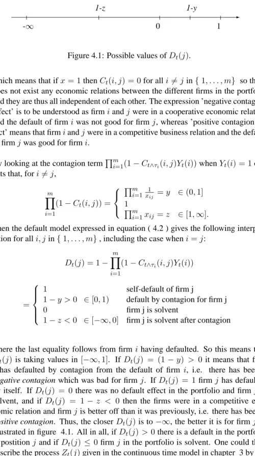
By assuming that the matrix C is time-independent and deterministic one can divide the m firms in the portfolio into fixed contagion classes. Firms belonging to the same contagion class need to satisfy the following:

1. Reflexivity:C(i, i) = 1for all i in{1, . . . , m}. 2. Symmetry: C(i, j) =C(j, i)for all i,j in{1, . . . , m_}.

3. Transitivity: C(i, h)C(h, j)_≤C(i, j)for all i,j,h in_{1, . . . , m_}. The contagion classes are disjoint and denoted by

[i] :={j ∈ {1, . . . , m} |C(i, j) = 1}

where it is assumed that the portfolio consists ofk_≤mcontagion classes[i1], . . . ,[ik].

The contagion classes might represent local markets. There can not be two differ-ent contagion classes defaulting at the same time, otherwise the two classes would actually be the same. Since the matrix C now is assumed to be time-independent and deterministic the portfolio default process in equation ( 3.1) becomes

Zt(j) =Yt(j) + (1−Yt(j)) 1₋Y i6=j (1₋C(i, j)Yt(i)) .

One sees thatZt(j) = 1ifYt(j) = 1andZt(j) = 1−Q_i₆₌_j(1−C(i, j)Yt(i))if

Yt(j) = 0. The contagion part

1−Qi₆=j(1−C(i, j)Yt(i))

= 1and gives default in the portfolio in positionjif there exists someisuch thatC(i, j)Yt(i) = 1. This

means that there must be at least one i in [j] in order to have a default in the portfolio in positionj. On the other hand, if1−Qi₆=j(1−C(i, j)Yt(i))

= 0

(38)

Yt(i) = 1andC(i, j) = C(j, i) = 0, by the symmetry assumption. This means

thatYt(i) = 0for alljin[i], and one gets that

Zt(i) = 0 ⇐⇒ Zt(j) = 0 for all j in [i],

which means that either all firms in the same contagion class have defaulted or that all firms are solvent. According to Biagini, Fuschini and Klüppelberg this form of classification of the firms makes their modeling different from usual credit risk contagion modeling since usual modeling would increase the default hazard of all the other firms in the same class when a default in that class occured. All firms belonging to the same contagion class[i]have a default intensity given by

λ[_ti]=X

j∈[i]

λj(t,Ψt).

Since the contagion matrix is assumed to be time-independent and deterministic, the default intensities of the portfolio default process,(Zt)t_≥0, are as the default

intensities of the self default indicator process(Yt(j))t≥0. The different contagion

classes are independent.

In the discrete time model all the firms and their enviroments were assumed to be fairly homogeneous, but they could not be put in the type of contagion classes described above since the contagion matrix is not symmetric. In the discrete time model the contagion matrix is deterministic and thecij which describes if there

exists a connection between the firmsiandjis symmetric and transient.

3.3.1 The default number

Like in the discrete time model, one can find the average number of defaulted firms within the portfolio. In the continuous time model, the default number process is linked to the contagion classes. All the firms in the portfolio are split into l _≤ m homogeneous groups, denoted byG1, . . . , Gl, where each group contains all the

firms that have the same default intensity. The groups might represent firms with identical credit rating (the probability of the issuer being able to pay its debt) or firms belonging to the same industry. For h in_{1, . . . , l_},Gh can be written as

the disjoint union of contagion classes, i.e.

Gh = sh

[

k=1

[j_kh]

wheresh is the number of contagion classes that groupGh consists of. Then the

weighted average number of defaults within groupGhis given by

mt(h) := 1 sh X i_∈[jh 1] Zt(i) nh 1 +. . .+ X i_∈[jh sh] Zt(i) nh sh (3.3)

(39)

wherenh

i is the cardinality of the contagion class[jih]for i in { 1, . . . , sh} and

mt:= (mt(1), . . . , mt(l)). Since the contagion classes are conditionally

indepen-dent of the filtration_Gt, by assumption in section 3.2, the summands of the process

mtare conditionally independent as well.

Recall that there can not be simultaneous defaults of contagion classes and all firms within a contagion class default at the same time. By following the reasoning of the proof of Lemma 3.4 in [11] one gets that, for h in_{1, . . . , l_}, the counting process

(mt)t≥0 will jump from a stateuinRlwithu = (u1, . . . , ul) =

(v1 s1, . . . , vl sl) : vh ∈ {0, . . . , sh}

to a state of the formu+eh

sh if and only if the next defaulting

firm belongs to groupGh. Theeh is the h-th element in the standard basis ofRl.

Theuh increases only in steps of _s1

h. The transition intensity ofmt(h) from the

state u into the stateu+eh

sh is given by λmt(h) t (u, u+ eh sh ) =sh(1−uh)λGh(t,Ψt) whereλGh(t,Ψ

t)is the default intensity of every firm belonging to groupGh, i.e.

the default intensiyt ofGh, anduhis the proportion of firms that have defaulted in

groupGhat time t.

The following example is ment to illustrate the contagion matrix and group struc-ture.

Example: Let there be two groups, Gi, i = 1,2, with 3 firms in one group and

4 firms in the other group. Let the contagion matrix be deterministic. Then the contagion matrix is as follows:

C=

C3×3 C3×4

C4×3 C4×4

LetI_d _{be the identity matrix in}_Rd_,0_d

×k be the zero matrix and let1d×k be the

matrix with only entries 1. Then one can consider the two following contagion cases: C1 = ₁ 3×3 03×4 0₄ ×3 14×4 C2= ₁ 3×3 03×4 1₄ ×3 I4×4

The interpretation of the case inC1 is that there is default contagion between the

3 firms in group 1, as well as it is contagion between the 4 firms in group 2. The zero matrices tells that there is no default contagin fromG1 and over toG2 and

no contagion the other way around either. The matrixC2models contagion within

G1, no default contagion fromG1 to G2, default contagin from group 2 over to

group 1 and no contagion within group 2. If the matrix C = 1₁₂

(40)

default contagion between all the 12 firms, and the caseC =I₁₂_{means that there}

is no default contagion between the firms. To explain the contagion effect in the case ofC2 a little bit more in detail, assume that the firms in groupG1 are called

a1, a2 anda3, and the firms inG2 are calledb1, b2, b3 andb4. Then13×3 means

that Ct(ai, aj) = 1 for all i, j = 1,2,3. I4×4 means that Ct(bi, bi) = 1 for

alli = 1,2,3,4. The case where 0₃

×4 tells thatCt(ai, bj) = 0 for all i, j, and

1₄

×3 means thatCt(bi, aj) = 1for alli, jas well as it has to include self default,

Ct(bi, bi) = 1.

3.4

The macroeconomic process

The macroeconomic processΨis chosen to be modeled as a one dimensional frac-tional Brownian motion, fBm, with Hurst indexH > 1₂, (See appendix B). Since the process is one dimensional it might be seen to represent a weighted mean of a vector of macroeconomic variables. The fBm was chosen to represent the macroe-conomic factors (such as supply and demand, unemploymentrate and inflation) since these factors often show a long range dependence. Since fBm is a long range time dependent process, it is not Markovian. The macroeconomic variable is given by

ΨH_t :=ψ(

Z t

0

g(s)dB_sH), t∈[0, T], (3.4) whereψis an invertible continuous function, and g is a deterministic function in Hµ([0, T])(see appendix B for more) such that _g₍1_s₎ is defined for all s in [0,T]. Sincegis a deterministic function the integral in equation ( 3.4) can be understood in a pathwise Riemann-Stieltjes sense by using the formula for integration by parts. (See page 124 in [1].)

Biagini, Fuschini and Klüppelberg restricted themself to the case where, for alli in{ 1, . . . , m} the default intensities of the self default processes(Yt(i))t≥0 are

stochastic and of the form λi(t,ΨH_t ) =βi(t)

Z t

0

g(s)dB_sH +γi(t), t_∈[0, T] (3.5) whereβiandγiare continuous functions.

The modeling choice of both [2] and [3] when it comes to the macroeconomic pro-cess is thus a zero mean Gaussian propro-cess. The disturbing element to the wealth process in equation ( 2.3) is decomposed into one term handling the macroeco-nomic factor and another term describing the individual fluctuations disturbing the wealth of a firm, whereas in the continuous time model only the macroeconomic factor is described explicitly. One big difference in the two models studied is re-garding the macroeconomic factor. In the discrete case, the macroeconomic factor

(41)

is constant over the time horizon of one year, but in the continuous model it is a stochastic process representing a mean of macroeconomic variables. The macroe-conomic process in the continuous time model is a fractional Brownina motion, so it is not a Markovian process. If the macroeconomic variable in the discrete time model was not constant, it would be Gaussian and thus a (standard) Brownian motion as well as it would be Markovian.

3.5

The price of credit derivatives

The prices of derivatives are influenced by the contagion matrix C and by the macroeconomic factorΨ. Before presenting the pricing formulas, there are some assumptions that need to be stated:

1. The information that the investor has at time t is given by_Ft, i.e. the investor

knows the processesΨ, the self default process Y and the contagion matrix C up to time t.

2. The default free interest rate is deterministic, and it is set equal to 0.

3. The risk neutral pricing measureQexists and is known such that the price at time t of anyFT-measurable claimLT inL1(Ω,Q)is given byEQ(LT|Ft) =

Ltfor0≤t≤T.

It is not assumed that the pricing measure necessarily is unique. Without the spe-cific expression of the macroeconomic processΨas given in equation ( 3.4), Bi-agini, Fuschini and Klüppelberg formulated the following pricing formula which is given without any restrictions on the matrix C, i.e. the matrix is stochastic and depends on time:

(42)

Theorem 1. Let f : R_×Rm _−→ R be a bounded measurable function. Let α = (α1, . . . , αm), β = (β1. . . , βm)andz = (z1, . . . , zm) be in{0,1}m and

h(i)_{, k}(i)_{be in}_{₀_,₁_}m−1 _{for i =}₁_{, . . . , m. Set}_h

ii =kii := 1for i =1, . . . , m,

hij := [h(i)]jandkij := [k(i)]j fori6=j. Then for t in [0,T]

E_Q(f(ΨT, ZT)|Ft) = X α,β,z∈{0,1}m (₋1)Pmj=1αjzj m Y j=1 z1−αj j × m Y i=1 (Yt(i)at(i))1−βi(1−Yt(i))βi EQ f(ΨT, z) m Y i=1 bt,T(i)βi|FtΨ , (3.6) with at(i) = X h(i)_∈{₀_,₁_}m−1 1 {h˜i(α,h)=0} 1 {C_τi(i)=h(i)_} bt,T(i) = X h(i)_,k(i)_∈{₀_,₁_}m−1 1 {C(_ti)=k(i)_} × Z ∞ T λi(u,Ψu)e− Ru t λ