A robust ranking method extending ELECTRE III to hierarchy of
interacting criteria, imprecise weights and stochastic analysis
Salvatore Correntea, Jos´e Rui Figueirab, Salvatore Grecoa,c, Roman S lowi´nskid,e
a
Department of Economics and Business, University of Catania, Corso Italia, 55, 95129 Catania, Italy
b
CEG-IST, Instituto Superior T´ecnico, Universidade de Lisboa, Av. Rovisco Pais, 1049-001 Lisboa, Portugal
c
University of Portsmouth, Portsmouth Business School, Centre of Operations Research and Logistics (CORL), Richmond Building, Portland Street, Portsmouth PO1 3DE, United Kingdom
d
Institute of Computing Science, Pozna´n University of Technology, 60-965 Pozna´n, Poland
e
Systems Research Institute, Polish Academy of Sciences, 01-447 Warsaw, Poland
Abstract:
A great majority of methods designed for Multiple Criteria Decision Aiding(MCDA) assume that all assessment criteria are considered at the same level, however, decision problems encountered in practice often impose a hierarchical structure of cri-teria. The hierarchy helps to decompose complex decision problems into smaller and manageable subtasks, and thus, it is very attractive for computational efficiency and ex-planatory purposes. To handle the hierarchy of criteria in MCDA, a methodology called Multiple Criteria Hierarchy Process (MCHP), has been recently proposed. MCHP per-mits to consider preference relations with respect to a subset of criteria at any level of the hierarchy. Here, we propose to apply MCHP to the ELECTRE III ranking method adapted to handle three types of interaction effects between criteria: mutual-weakening, mutual-strengthening and antagonistic effect. We also involve in MCHP an imprecise elicitation of criteria weights, generalizing a technique called the SRF method. In order to explore the plurality of rankings obtained by the ELECTRE III method for possible sets of criteria weights, we apply the Stochastic Multiobjective Acceptability Analysis (SMAA) that permits to draw robust conclusions in terms of rankings and preference relations at each level of the hierarchy of criteria. The novelty of the whole methodology consists of a joint consideration of hierarchical assessments of alternatives performances on interacting criteria, imprecise criteria weights, and robust analysis of ranking recom-mendations resulting from ELECTRE III. An example regarding the multiple criteria ranking of some European universities will show how to apply the proposed methodology on a decision problem.
Keywords: Multiple Criteria Hierarchy Process, ELECTRE III method, SRF method,
Stochastic Multiobjective Acceptability Analysis
1. Introduction
Scientific decision aiding is confronted with more and more complex decision problems in various domains of our society, such as environmental management, health care, homeland security, among others. The complexity of these problems is mainly related to the number and the heterogeneity of objectives to be obtained. To deal with these types of problems in an effective way, Multiple Criteria Decision Aiding (MCDA) provides methods that work-out recommendations consistent with
Email addresses: [email protected](Salvatore Corrente),[email protected](Jos´e Rui Figueira), [email protected](Salvatore Greco),[email protected](Roman S lowi´nski)
the preferences of the Decision Maker (DM) [12]. Analysis of the current trends in MCDA leads to the conclusion that the following concerns become more and more relevant in this field:
1. Consideration of a great number of assessment criteria: The number of criteria is a factor un-derlying the complexity of decision problems. The criteria representing different points of view on the quality of alternatives are usually in conflict, because alternatives which are good on some criteria are frequently bad on some other criteria. This makes the search of a compromise among criteria more difficult when the number of criteria is growing [18]. A practical way to cope with the high dimensionality of multiple criteria performances assessment is the hierar-chical decomposition of the family of criteria [7]. It permits not only to reduce the number of criteria which contribute to the assessment of alternatives from a specific higher-level point of view, but also to group criteria into logically consistent sub-families. The hierarchical structur-ing of the family of criteria also facilitates the elicitation of preferences by the DM who is no more obliged to make comparisons of large “vectors” of heterogeneous performances, but can express the preferences with respect to some meaningful subsets of criteria. The DM appreci-ates, moreover, a final recommendation (in terms of a ranking or a preference relation in the set of alternatives) not only with respect to the whole family of criteria, but also with respect to some sub-criteria located at lower levels of the hierarchy. The above benefits of the hierarchical decomposition, in the sense of preference elicitation and final recommendation, motivated the elaboration of the methodology called Multiple Criteria Hierarchy Process (MCHP) [7]. 2. Consideration of interaction between criteria: Indeed, it is highly probable that among the
many assessment criteria considered in a decision problem, there are interacting criteria in the sense of some mutual-weakening effects, mutual-strengthening effects, or antagonistic effects, as will be explained in subsection 2.2. Different methodologies have been proposed to take into account interaction between criteria, such as non-additive integrals, with the best known Cho-quet integral for cardinal criteria, and Sugeno integral for ordinal ones [4, 31], some augmented additive value functions [14], and some extended outranking models [9].
3. Acceptance of intransitivity or incompleteness in the recommended ranking of the alternatives: In fact, forcing the transitivity and completeness by methods grounded in the Multiple At-tribute Value Theory (MAVT) [18], can lead to induce some preferences that are not well founded. Some alternatives may simply be incomparable because of very contrasted perfor-mances on the conflicting criteria. The transitivity of an indifference relation is also doubtful, as shown by the famous example of the transitivity of indifference spanned over a series of similar cups of coffee [21]. For these reasons outranking methods, such as ELECTRE and PROMETHEE have been proposed [3, 10] (see [15] for a recent extension of the ELECTRE methods to group decision-making under fuzzy environment). These methods make use of an outranking relation S as a preference model, such thataSbif “alternative a is at least as good as alternative b”. Thus, if neither aSb nor bSa is true, then a and b are incomparable. The outranking relations are supposed to be only reflexive, i.e., neither complete nor transitive. 4. Consideration of robustness concerns related to non-univocal values of preference model
param-eters: The recommendation supplied by any MCDA method depends on the values assigned to preference model parameters (e.g., weights and veto thresholds); when these values are not univocal (e.g., when many sets of weights and/or thresholds are possible), then it is advisable to identify more and less stable parts of the recommendation. For example, some alternatives may keep the same position in the ranking even if the preference model parameters change in a large interval of possible values, while the position of other alternatives may be much more sensitive to the change of the same model parameters. The range of the changes of a given recommendation is, obviously, an important information for the DM - it gives account of the robustness of this recommendation [25]. In this view, two main approaches have been
developed within MCDA: Stochastic Multiattribute Acceptability Analysis (SMAA) [19] and Robust Ordinal Regression (ROR) [6]. SMAA samples the space of variability of the considered preference model parameters and, in this context, supplies the frequency with which a given alternative is preferred, indifferent or incomparable to another one. ROR, instead, takes into account all sets of preference model parameters compatible with the preference information provided by the DM, and defines the necessary preference relation, in case an alternative is preferred to another one for all the sets of compatible preference model parameters, as well as the possible preference relation, in case an alternative is preferred to another one for at least one set of compatible preference model parameters.
The above four issues are very often present in the same real-life multiple criteria decision problem. There exist methods able to deal with problems where some of these issues are present, however, the MCDA literature does not provide any proof of a joint consideration of all these issues. Consequently, the aim of this paper is to provide a methodology of MCDA that fills this gap. It is worth stressing that elaboration of the comprehensive methodology does not consist of a simple sequential application of the existing methods coping with each particular issue. These issues are interrelated and this requires a careful adaptation of the methods contributing to the comprehensive methodology.
More specifically, we propose to apply MCHP to the ranking method ELECTRE III adapted to handle three types of interaction between criteria: mutual-weakening effect, mutual-strengthening effect, or antagonistic effect. Moreover, we introduce in MCHP an imprecise elicitation of criteria weights, generalizing a technique called the SRF method [11]. Then, to explore the plurality of partial preorders obtained by the ELECTRE III method for possible sets of criteria weights, we apply SMAA that permits to draw robust conclusions in terms of frequency of preference, indifference and incomparability relations at each level of the hierarchy of criteria.
The plan of the article is the following. In Section 2, we recall some basic concepts and methods that contribute to the proposed methodology. This creates a background for next sections where we develop our proposal. A new version of the SRF method handling an imprecise information received from the DM is described in Section 3. In Section 4, we describe the complete methodology, and then, we illustrate its application using a case study presented in Section 5. Section 6 contains conclusions and perspective directions of research.
2. Background
2.1. The Multiple Criteria Hierarchy Process (MCHP)
The MCHP has been introduced in [7] to deal with decision problems where assessment criteria are not considered at the same level but they are organized in a hierarchical way, as shown in Figure 1.
Figure 1: Example of a hierarchy of criteria
• G0 is the root of the hierarchy, and it represents the global objective,
• G is the set of all criteria in the hierarchy, while IG denotes the set of indices of all criteria in
the hierarchy,
• EL is the set of indices of all elementary criteria, that are the criteria located at the bottom of the hierarchy,
• Gr, wherer∈ IG, is a generic criterion in the hierarchy, while ifr∈ IG\EL, thenG(r,1), . . . , G(r,n(r))
are the subcriteria of Gr located at the level immediately below,
• for all r∈ IG\EL,E(Gr) represents the set of all elementary criteria descending from criterion
Gr. In the following, a criterion Gr, such that r ∈ IG \EL, will be called non-elementary
criterion.
2.2. The hierarchical ELECTRE III method with interactions between criteria
In order to apply the ELECTRE III method in conjunction with the MCHP, one needs to get from the DM some preference information in terms of the values of preference model parameters: weights of the elementary criteria, and veto thresholds on these criteria. For each elementary crite-rion gt,t∈EL, a weight representing its relative importance within the family of elementary criteria
is denoted by wt. The weights are supposed to be positive and normalized, that is, wt>0 for each
t ∈EL and X
t∈EL
wt = 1. Moreover, for each t ∈EL and for each a belonging to the set of
alterna-tives A, the following thresholds should be specified: indifference qt(a), preference pt(a), and veto
vt(a) thresholds. The indifference threshold is the maximum difference between the performances
of alternatives a and b on gt compatible with their indifference on gt; the preference threshold is
the minimum difference between the performances of a and b on gt compatible with the preference
of one over the other on gt; the veto threshold represents the minimum difference between the
per-formances of b over a on gt incompatible with the outranking of a over b on any criterion Gr from
which gt is descending, that is, t ∈ E(Gr). In the following, for the sake of simplicity, but without
loss of generality, we shall suppose that the thresholds are not dependent on the performances of the alternatives. Consequently, we shall writeqt, pt andvtinstead of qt(a),pt(a) and vt(a), respectively.
ELECTRE III [23] builds a fuzzy outranking relation in the set of alternatives, representing the credibility that an alternative is at least as good as another one. The construction involves concor-dance and discorconcor-dance indices concerning the hypothesis that one alternative is at least as good as (outranks) another one. The concordance index represents the strength of the coalition of criteria being in favor of the hypothesis that a outranks b (a, b ∈ A), and the discordance indices repre-sent opposition of criteria being discordant with this hypothesis. In order to perform these tests and calculate the credibility of outranking that aggregates concordance and discordance, one has to calculate for each pair of alternatives (a, b)∈A×A the following indices [8]:
• the elementary concordance index, for each elementary criterion gt,
ϕt(a, b) = 1 if gt(b)−gt(a)≤qt, (aStb) pt−[gt(b)−gt(a)] pt−qt if qt< gt(b)−gt(a)< pt, (bQta) 0 if gt(b)−gt(a)≥pt, (bPta). (1)
• the elementary discordance index, for each elementary criterion gt,
dt(a, b) = 1 if gt(b)−gt(a)≥vt, [gt(b)−gt(a)]−pt vt−pt if pt< gt(b)−gt(a)< vt, 0 if gt(b)−gt(a)≤pt, (2)
• the partial concordance index for each non-elementary criterion Gr, Cr(a, b) = X t∈E(Gr) wtϕt(a, b) X t∈EL wt (3)
• the partial credibility index for each non-elementary criterion Gr,
σr(a, b) = Cr(a, b) Y n t∈E(Gr) :dt(a, b)> Cr(a, b) o 1−dt(a, b) 1−Cr(a, b) . (4)
In view of the above formulas, observe that in order to avoid that only one immediate subcriterion ofGrdecides about outranking (Sr) or non-outranking (Src) for any pair of alternatives (a, b)∈A×A,
even without imposing the veto, it is reasonable to impose a condition that no weight W(r,j) of
subcriterion G(r,j), j = 1, ..., n(r), is greater than the sum of weights of the remaining immediate
subcriteria of Gr, i.e., W(r,j) ≤ n(r) X k=1 k6=j W(r,k). (5)
Otherwise, subcriterion G(r,j) would be a dictator in relation to Gr. For this reason, below, we
call condition (5) a non-dictatorship condition [26].
In some cases, three types of interactions could be observed between criteria. Given an elementary criterion gt1 being in favour of the outranking of a overb, then [9]:
• if gt2 is also in favour of the outranking of a over b, we say thatgt1 and gt2 present a
mutual-strengthening effect when the importance assigned to the set composed of the two elementary criteria considered together is greater than the importance assigned to the two elementary criteria considered separately; in this case, a value wt1t2 >0 has to be added to the sum of the
weights wt1 +wt2 when computing the concordance index,
• if gt2 is also in favour of the outranking of a over b, we say thatgt1 and gt2 present a
mutual-weakening effect when the importance assigned to the set composed of the two elementary criteria considered together is lower than the importance assigned to the two elementary criteria considered separately; in this case, a value wt1t2 <0 has to be added to the sum of the weights
wt1 +wt2 when computing the concordance index,
• if gt2 is opposing to the outranking of a over b, we say thatgt2 presents an antagonistic effect
over gt1 when the importance assigned to gt1 has to be lowered by the opposition of gt2. In
this case, a value wt′1t2 > 0 has to be subtracted from the weight wt1 when computing the
concordance index.
Let us precise that the contribution given by each criterion to the credibility of the outranking of one alternative over another could not be negative. Therefore, the following net flow condition has to be fulfilled: Condition 2.1. (see [9]) For all t1 ∈EL, wt1 − X t2∈EL:wt1t2<0 |wt1t2|+ X t3∈EL wt′1t3 ≥0. (6)
Let us denote by C(bHa) the set of all elementary criteria such that bHa, where H ∈ {S, Q, P}
and by C(bHa) its complement. C(bP a) represents the set of elementary criteria that do not oppose too strongly to the outranking of a over b and, consequently,C(bP a) =C(aSb)∪C(bQa).
Given a non-elementary criterion Gr, and the possible interactions between the elementary criteria,
the partial concordance index Cr(a, b) can be rewritten as follows:
Cr(a, b) = 1 Wr(a, b) X t1∈C(bP a)∩E(Gr) wt1ϕt1(a, b) + X t1,t2∈C(bP a)∩E(Gr) wt1t2Z(ϕt1(a, b), ϕt2(a, b))− − X t1∈C(bP a)∩E(Gr), t2∈C(bP a)∩E(Gr) wt′1t2Z(ϕt1(a, b), ϕt2(a, b)) (7) where Wr(a, b) = X t∈E(Gr) wt+ X t1,t2∈C(bP a)∩E(Gr) wt1t2Z(ϕt1(a, b), ϕt2(a, b))− − X t1∈C(bP a)∩E(Gr), t2∈C(bP a)∩E(Gr) wt′1t2Z(ϕt1(a, b), ϕt2(b, a))
and Z : [0,1]2 →[0,1] is a non-decreasing function of its arguments, such thatZ(1, x) = Z(x,1) =x
for all x∈[0,1]. In the following, we shall consider Z(x, y) = xy.
2.2.1. Ascending and Descending distillations
The final partial preorder of alternatives produced by the ELECTRE III method is obtained as the “intersection” of two complete preorders that are the results of the so-called descending and ascending distillations [23]. In the descending distillation, one orders the alternatives from the best to the worst, while in the ascending distillation, one orders the alternatives in the opposite way, starting from the worst and finishing with the best.
Given a non-elementary criterion Gr, and λk ∈ [0,1], both distillations concern the following fuzzy outranking relation:
aSλk r b⇔ σr(a, b)> λk, σr(a, b)> σr(b, a) +s(σr(a, b)), (8) where s(λ) =αλ+β and, following [23], α=−0.15 andβ = 0.3.
For each alternative a, and each non-elementary criterionGr, its λk-qualification with respect toGr
is obtained as follows: qλk r,A(a) = p λk r,A(a)−f λk r,A(a) (9) where • pλk r,A(a) = | b∈A:aSλk
r b | is the λk-power of a; it is the number of alternatives that are
outranked by a onGr, • fλk
r,A(a) =|
b∈A:bSλk
r a |is theλk-weakness ofa; it is the number of alternatives outranking
Algorithm 1 Descending distillation
Input: Credibility of outranking σr(a, b) for a given non-elementary criterion Gr, and all a, b∈A.
Output: Ordered classes of alternatives C1 ≻ C2 ≻ . . . ≻ Cn, such that ∪ni=1Ci = A, where ≻ denotes strict preference relation,
1. n= 0, A0 =A, (A0 contains all alternatives that have not yet been assigned),
2. λ0 = max
a,b∈An, a6=b
{σr(a, b)},
3. k= 0, D0 =An,
4. λk+1 = max
{(a,b):σr(a,b)<λk−s(λk), a,b∈Dk}
{σr(a, b)};
if {(a, b) : σr(a, b)< λk−s(λk), a, b∈Dk}=∅, then λk+1 = 0,
5. Calculate the λk+1-qualifications of all the alternatives belonging to Dk with respect to Gr,
6. Obtain the maximum λk+1-qualification qr,Dk = max
a∈Dk
n
qλk+1
r,Dk(a)
o
7. Build the subset:
Dk+1 ={a∈Dk :q λk+1 r,Dk(a) =qr,Dk} 8. if |Dk+1|= 1 or λk+1 = 0 go to step 9. else k =k+ 1, Dk =Dk and go to step 4. endif 9. Cn+1 =Dk+1, An+1 =An\Cn+1, if An+1 6=∅ n =n+ 1, go to step 2. else
end of the distillation.
Algorithm 2 Ascending distillation
Input: Credibility of outranking σr(a, b) for a given non-elementary criterion Gr, and all a, b∈A.
Output: Ordered classes of alternatives C1 ≻ C2 ≻ . . . ≻ Cn, such that ∪ n
i=1Ci = A, where ≻ denotes strict preference relation,
1. n= 0, A0 =A, (A0 contains all alternatives that have not yet been assigned),
2. λ0 = max
a,b∈An, a6=b
{σr(a, b)},
3. k= 0, D0 =An,
4. λk+1 = max
{(a,b):σr(a,b)<λk−s(λk), a,b∈Dk}
{σr(a, b)};
if {(a, b) : σr(a, b)< λk−s(λk), a, b∈Dk}=∅, then λk+1 = 0,
5. Calculate the λk+1-qualifications of all the alternatives belonging to Dk with respect to Gr,
6. Obtain the minimum λk+1-qualification qr,Dk = mina∈Dk
n
qλk+1 r,Dk(a)
o
7. Build the subset:
Dk+1 ={a∈Dk :q λk+1 r,Dk(a) =qr,Dk} 8. if |Dk+1|= 1 or λk+1 = 0 go to step 9. else k =k+ 1, Dk =Dk and go to step 4. endif 9. Cn+1 =Dk+1, An+1 =An\Cn+1, if An+1 6=∅ n =n+ 1, go to step 2. else
end of the distillation.
The algorithms for the descending and ascending distillation are described in detail as Algorithm 1 and Algorithm 2, respectively [2].
In each of the distillations the alternatives are ordered in classes, and each class contains at least one alternative. Therefore, the final preorder is obtained as the intersection of the two distillations. Given a, b∈A and a non-elementary criterion Gr,
• a is preferred to b on Gr (aPrb), if a belongs to a class not worse than that of b in both
distillations, and to a better class for at least one of the two distillations,
• a is indifferent to b onGr (aIrb), ifa and b belong to the same class in both distillations, • a and b are incomparable on Gr (aRrb), ifa belongs to a class better thanb in one distillation
and worse in the other one.
2.3. The SRF method
As described in subsection 2.2, the application of the ELECTRE III method necessitates the knowledge of weights of the elementary criteria. One can get these weights in two ways: receiving the weights directly from the DM, or using an indirect preference information provided by the DM from which some weights compatible with this information are inferred. In the second way, the Simos method has been proposed in [27, 28], modified later in [11], and implemented in the software called SRF. Hence, we call here the implemented method by the same name - the SRF method.
In the following, we describe the application of the SRF method to the set composed of elementary criteria only. Let us remind that the application of the SRF method to the case of criteria structured in a hierarchical way has been introduced in [5].
In the SRF method, the DM is asked to rank the elementary criteria with respect to their relative importance from the least important, belonging to the subset L1 ⊆ EL, to the most important,
belonging to the subset Lv ⊆ EL. Moreover, the DM can insert some blank cards between two successive subsets of criteriaLsandLs+1 to increase the difference of importance between elementary
criteria inLsand inLs+1. The number of blank cards included between subsets of elementary criteria Ls and Ls+1 is denoted by es. Finally, the DM is asked to provide a ratioz between the importance
of elementary criteria in Lv and the importance of elementary criteria in L1.
From a formal point of view, following [5], the non-normalized weight of elementary criterion gt
is computed as w′t= 1 + (z−1) l(t)−1 + l(t)−1 X s=1 es v−1 + v−1 X s=1 es
where l(t) represents the rank to which elementary criterion gt belongs, that is t ∈ Ll(t).
Con-sequently, the normalized weight wt assigned to each elementary criterion t ∈ EL is obtained as
follows: wt= wt′ X t∈EL w′t .
2.4. The Stochastic Multiobjective Acceptability Analysis (SMAA)
The SMAA methodology has been presented for the first time in [19] in order to deal with decision problems where evaluations of alternatives on criteria, and some preference model parameters are not precisely known. SMAA can be considered as a way of handling robustness concerns related to
preference model parameters and performances of alternatives on the considered criteria. Below, we remind the main features of SMAA without assuming any specific preference model (for a survey of the SMAA methods see [32], while for a real-world application of SMAA see [33]). In SMAA two probability distributions, denoted by fW and fχ, are defined on W and the performance space
χ = [gj(a)|j = 1, . . . , m, anda ∈A]. SMAA is based on sampling of both weight and performance
spaces. Depending on the chosen preference model various indices can be used to summarize the sampling results. For preference model being a value function (providing a complete ranking of the alternatives), the rank acceptability index bl(a) and thecentral weight vector wc(a) can be computed for eacha∈Aand for each rank positionl= 1, . . . , n. bl(a) gives the frequency with which alternative
a takes the l-th position in the final ranking, while wc(a) specifies the average weight vector giving to alternative a the best position in the final ranking.
For a preference model being a value function or an outranking relation, the pairwise winning index P re(a, c) gives the frequency with which alternativea is preferred to alternative c[20]
P re(a, c) = Z w∈W fW(w) Z ξ∈χ:a≻Mc fχ(ξ)dξ dw
wherea≻M cis the preference relation provided by the model compatible with the DM’s preferences.
3. The imprecise SRF method
As already observed in [29], the SRF method produces a single set of criteria weights while, in general, there exists an infinity of the sets of weights compatible with the preference information provided by the DM. For this reason, the authors of [29] proposed different ways of handling the plurality of sets of the weights compatible with the preference information provided by the DM. In the present paper, our aim is quite different, since we propose a new variant of the SRF method that takes into account a different type of imprecision. This imprecision is not only related to the plurality of sets of weights compatible with the preference information provided by the DM but it is also related to the imprecision of this information.
As explained in subsection 2.3, in order to apply the SRF method, the DM is asked to:
1) rank the criteria from the least important to the most important with the possibility of ex aequo between them,
2) put some blank cards between two successive subsets of criteria to increase the difference of importance between criteria in these two subsets,
3) define the ratio z between the importance of the most important subset of criteria and the importance of the least important one.
We suppose that the imprecision of the information provided by the DM regards points 2) and 3). Indeed, in our opinion, when applying the SRF method, it is quite reasonable to suppose that the DM may provide, on one hand, an imprecise number of blank cards between two successive subsets of criteria and, on the other hand, an imprecise importance ratio z.
In the following, first we describe the imprecise SRF method on a set of generic criteria {g1, . . . , gm}, after we extend the method to the case of a set of weights organized in a hierarchy.
Let us suppose that the DM claims that criteria in Ls+1 are more important than criteria in Ls but, she is not sure about the number of blank cards that should be included between the two subsets of criteria, that is, about the value of es. Consequently, she states that es ∈ [lows, upps] where, lows ≤ upps. In this way, denoting the weights of criteria in Ls and Ls+1 bywLs and wLs+1,
respectively, and denoting by C the importance of a blank card included betweenLs and Ls+1, the
preference information provided by the DM can be translated to the following pair of constraints: wLs+1 ≥wLs + (lows+ 1)·C, wLs+1 ≤wLs + (upps+ 1)·C, C > 0.
Analogously, it is possible that, the DM is unsure about the ratiozbetween the criteria inLv and the criteria in L1. For this reason, she may wish to provide an interval of possible values to which z
should belong. This means that z ∈ [zlow, zupp]. Denoting by wL1 and wLv the weight of a criterion
belonging to L1 and Lv, respectively, this piece of preference information can be easily translated to the constraints
zlow ≤
wLv wL1
≤zupp⇔zlow·wL1 ≤wLv ≤zupp·wL1.
Therefore, the set of constraints translating the above preference information provided by the DM is the following: wLs+1 ≥wLs + (lows+ 1)·C, wLs+1 ≤wLs + (upps+ 1)·C, C >0, for all s= 1, . . . , v−1, zlow ·wL1 −wLv ≤0, wLv −zupp·wL1 ≤0, wL1 >0 (10)
while to normalize the weights of criteria, the following constraint should also be included: v
X
i=1
|Li| ·wLi = 1.
If the imprecise SRF method is applied to a flat structure of criteria, the non-dictatorship condi-tion (5) should be appended to the constraints (10) if Lv would be composed of only one criterion, and only for this criterion. This is because only if Lv is a singleton, this criterion could become a dictator. Therefore, the constraint that should be appended to (10) in this case is the following:
wLv ≤
v−1
X
s=1
wLs · |Ls|.
Let us observe that the DM can consider the whole set W of weights satisfying the constraints of the imprecise SRF method, but she can also select one representative set of weights, for example the barycenter of W.
Example 3.1. Let us suppose that the DM considers 8 criteria {g1, . . . , g8} and that she provides
the following preference information:
• the criteria are ordered from the least important to the most important ones in the following subsets: L1 ={g6}, L2 ={g5, g7}, L3 ={g1, g3}, and L4 ={g2, g4},
• the number of blank cards between L1 and L2 should belong to [1,3], there is one blank card
between L2 and L3 and the number of blank cards between L3 and L4 should belong to [2,4], • the importance ratio between criteria in L4 and the criteria in L1 should belong to the interval
According to (10), the preference information provided by the DM is translated to the following set of constraints: wL1 + 2C ≤wL2 ≤wL1 + 4C, wL3 =wL2 + 2C, wL3 + 3C ≤wL4 ≤wL3 + 5C, 2·wL1 ≤wL4 ≤4wL1, C > 0, wL1 >0, wL1 + 2·wL2 + 2·wL3 + 2·wL4 = 1.
where w6 = wL1, w5 = w7 = wL2, w1 = w3 = wL3, and w2 = w4 = wL4. Whichever vector
of weights (wL1, wL2, wL3, wL4) satisfying the above set of constraints is therefore compatible with the
preference information provided by the DM. For example, a feasible solution is wL1 = 0.06,wL2 = 0.1, wL3 = 0.15and wL4 = 0.22. Let us underline that, as explained above, in this case it is not necessary
to take into account the non-dictatorship condition since two criteria are in the most important subset.
In order to adapt the proposed imprecise SRF method to the case of criteria structured in a hierarchical way, the DM is therefore asked to apply the imprecise SRF method on each subset of criteria {G(r,1), . . . , G(r,n(r))} composed of the immediate subcriteria of the non-elementary criterion
Gr. It will be enough to perform the following replacements in the notation of the imprecise SRF
method described above:
• L1, . . . , Lv with Lr1, . . . , L r v, • wL1, . . . , wLv with W r L1, . . . , W r Lv, • es with ers,
• [lows, upps] with [low
r s, upp r s], • z with zr ,
• [zlow, zupp] with zr low, z r upp .
Therefore, in applying the imprecise SRF method to the set of criteria {G(r,1), . . . , G(r,n(r))}, the set
of constraints in (10) will be replaced by the following one:
Er WLr s+1 ≥WLrs + (low r s+ 1)·Cr, WLr s+1 ≤WLrs + (upp r s+ 1)·Cr, Cr>0, for all s= 1, . . . , v−1, zr low·WLr 1 −WL r v ≤0, WLr v−z r upp·WLr 1 ≤0, WLr 1 >0. (11)
Two more points should be underlined:
1. According to [5], the weight Wr of each non-elementary criterion Gr, can be obtained as the
sum of the weights of the elementary criteria descending from Gr, that is
Wr =
X
t∈E(Gr)
Consequently, the constraints translating the preference information provided by the DM during the application of the imprecise SRF method on the subset of criteria{G(r,1), . . . , G(r,n(r))}, can
be expressed in terms of the weights of the elementary criteria only.
2. The value of Cr appearing in the set of constraints (11) and representing the importance of a
blank card inserted between two successive subsets of criteria, is not the same whichever crite-rion in the hierarchy is considered. For example, if the criteria are structured in a hierarchical way as in Figure 1, then a blank card inserted between criteria G1 and G2 is not necessarily as
important as a blank card inserted between elementary criteria g(2,3) and g(2,2) at the bottom
level of the hierarchy.
Example 3.2. Let us suppose that the DM is interested in obtaining the weights of criteria structured
in a hierarchical way as shown in Figure 1. For this reason, she applies the imprecise SRF method at first on the set of criteria {G1, G2, G3}, and then, on the sets of criteria
g(1,1), g(1,2), g(1,3) , {g(2,1), g(2,2), g(2,3), g(2,4)}and {g(3,1), g(3,2), g(3,3)}, separately. In the following, we shall show in detail
the application of the imprecise SRF method to the sets of criteria{G1, G2, G3}and{g(3,1), g(3,2), g(3,3)}
only.
• Regarding the first level criteria, the DM states that G2 =L01 is less important than G1 = L 0 2
that is less important than G3 = L03. She says that the number of blank cards e 0
1 between G2
and G1 belongs to the interval [2,3] = [low 0
1, upp
0
1], while the number of blank cards e 0
2 between G1 and G3 belongs to the interval [1,2] = [low
0
2, upp
0
2]. Moreover, the importance ratio z 0
between G3 and G2 belongs to the interval [1,3] =
z0 low, z 0 upp . Consequently, denoting by C0
the importance of a blank card inserted between two successive subsets of criteria, the set of constraints translating these preferences is the following:
E0 WL0 1 + 3C0 ≤WL 0 2 ≤WL 0 1 + 4C0, WL0 2 + 2C0 ≤WL 0 3 ≤WL 0 2 + 3C0, WL0 1 ≤WL 0 3 ≤3WL 0 1, WL0 1 >0, C0 >0. → X t∈E(G2) wt+ 3C0 ≤ X t∈E(G1) wt ≤ X t∈E(G2) wt+ 4C0, X t∈E(G1) wt+ 2C0 ≤ X t∈E(G3) wt ≤ X t∈E(G1) wt+ 3C0, X t∈E(G2) wt ≤ X t∈E(G3) wt ≤3 X t∈E(G2) wt, X t∈E(G2) wt >0, C0 >0. (13)
• Regarding the subset of elementary criteria {g(3,1), g(3,2), g(3,3)}, let us suppose that the DM
states that g(3,1) = L 3
1 is less important than g(3,3) = L 3
2 that, in turn, is less important than g(3,2) =L33. She says that the number of blank cards e
3
1 between g(3,1) and g(3,3) should belong
to the interval [1,2] = [low3
1, upp
3
1], while the number of blank cards e 3
2 between g(3,3) and g(3,2)
should belong to the interval [2,3] = [low3 2, upp
3
2]. Moreover, the importance ratio z 3
between
g(3,2) and g(3,1) should belong to the interval [1,4] =
z3 low, z 3 upp . As a consequence, denoting by C3 the importance of a blank card inserted between two successive subsets of criteria, this
preference information can be translated into the following set of constraints: E3 WL3 1 + 2C3 ≤WL 3 2 ≤WL 3 1 + 3C3, WL3 2 + 3C3 ≤WL 3 3 ≤WL 3 2 + 4C3, WL3 1 ≤WL 3 3 ≤4WL 3 1, WL3 1 >0, C3 >0. → w(3,1)+ 2C3 ≤w(3,3) ≤w(3,1)+ 3C3, w(3,3)+ 3C3 ≤w(3,2) ≤w(3,3)+ 4C3, w(3,1) ≤w(3,2) ≤4w(3,1), w(3,1) >0, C3 >0. (14)
In order to adapt the condition of non-dictatorship (5) when using the imprecise SRF method to criteria structured hierarchically, we have to take into account two special cases:
case 1) No information is provided by the DM about relative importance of criteria immediately de-scending from non-elementary criterionGr. In this case, for each j = 1, . . . , n(r), the following
constraint should be added:
W(r,j) ≤ n(r) X k=1 k6=j W(r,k);
case 2) The DM provided information about relative importance of criteria immediately descending from non-elementary criterion Gr. In this case, the non-dictatorship condition should be
in-cluded only if a single criterion has been indicated as the most important among the immediate descending of Gr. Then, the non-dictatorship condition is the following:
N Dr WLr v ≤ v−1 X s=1 WLr s−1 · |L r s−1|, WLr
s =W(r,j), for all s= 1, . . . , v−1, and for all G(r,j) ∈L r
s.
As in this paper we are considering a hierarchy of interacting criteria, the complete set of con-straints defining the weights of the elementary criteria and the coefficients representing the possible interactions between elementary criteria is the following:
E [1] ∪r∈IG\EL{Er∪N Dr}, [2]
wt1,t2 >0 if elementary criteria gt1 and gt2 present a mutual-strengthening effect,
wt1,t2 <0 if gt1 and gt2 present a mutual-weakening effect,
w′t1t2 >0 if gt2 presents an antagonistic effect over gt1,
[3] wt1 − X t2∈EL:wt1t2<0 |wt1t2|+ X t3∈EL wt′1t3
≥0, for all t1 ∈EL,
[4] X t∈EL wt= 1, [5] X {t1,t2}⊆EL: wt1t2>0 wt1t2 ≤ X t∈EL wt.
In E, constraints [1] translate the information provided by the DM during the application of the imprecise SRF method on each subset of criteria {G(r,1), . . . , G(r,n(r))} and include possibly the
Constraints [2] translate the preference information provided by the DM in terms of possible inter-actions between elementary criteria, while constraints [3]-[5] are technical constraints. In particular, constraints [3] ensure that the contribution given by each elementary criterion to the credibility of outranking is non-negative; constraint [4] is a normalization constraint, while constraint [5] is intro-duced to limit the importance assigned to the mutual-strengthening effects. Indeed, in this way, the sum of the coefficients representing the mutual-strengthening effects between the elementary criteria cannot be more important than the unanimity of the elementary criteria.
Let us underline that the methodology does not exclude some additional constraints on the weights if the DM is willing to express them. For example, independently from the application of the SRF method she could claim that a criterion is more important that the sum of others, or that the weight assigned to a criterion has not to be lower than a certain threshold. In those cases, the corresponding constraints have to be added to the set E.
4. The proposed methodology
The set of constraints E defines a space composed of an infinite number of vectors of weights and interaction coefficients compatible with the preference information provided by the DM. In the following, we call such a vector a compatible vector. For existence of many compatible vectors, we propose to apply the SMAA methodology. SMAA permits to get robust recommendations by exploring the different partial rankings resulting from the application of the hierarchical ELECTRE III method with interactions on a large sample of compatible vectors.
The flow chart describing the proposed method is shown in Figure 2 and it is composed of the following steps:
Step 0 Fix the hierarchical structure of the set of criteria using the MCHP, distinguishing the
subsets of elementary criteria, and higher level criteria, up to the root criterion.
Step 1 The DM, or the analyst representing the DM, is asked to provide different types of preference
information:
1.1 Indifference, preference and veto thresholds for each elementary criterion.
1.2 Information about possible mutual-strengthening and mutual-weakening effects, as well as about the possible antagonistic effects between some elementary criteria.
1.3 Information required by the imprecise SRF method for each subset of criteria{G(r,1), . . . , G(r,n(r))}
and each non-elementary criterion Gr.
Step 2 The analyst has to check if there exists at least one compatible vector. From a computational
point of view, this means that one has to solve the following LP problem:
ε∗ = maxε, s.t. E′ =h1′i∪h2′i∪h3′i∪[4]∪[5] (15)
where the sets of constraints 1′
, 2′
, and 3′
are obtained from [1], [2], and [3] by transform-ing strict inequalities into weak inequalities ustransform-ing an auxiliary variable ε (for example, C0 >0
is transformed into C0 ≥ε).
If the set of constraints E′ is feasible and ε∗ > 0, then there exists at least one compatible vector. In the opposite case (E′ is infeasible orε∗ ≤0), there is some inconsistency in the pref-erence information provided by the DM that can be identified by using some of the techniques proposed in [22] (Step 2.1). Once this inconsistency is removed, one can pass to the next step.
Figure 2: Flow chart of the proposed methodology
Step 3 As there may exist many compatible vectors, we suggest to sample them. Since set E′ is
composed of linear constraints and they define a convex space, one can use the Hit-And-Run (HAR) method proposed in [30] and recently revisited in [34] and [35].
Step 4 For each sampled compatible vector and for each non-elementary criterionGr, one performs
the descending and the ascending distillations of the credibility of outranking, giving descend-ing and ascenddescend-ing complete preorders, respectively. Their intersection gives a partial preorder of the alternatives. Consequently, as observed in Section 2.2.1, the preference (Pr), indifference
(Ir) and incomparability (Rr) relations are known for each compatible vector and for each
non-elementary criterion Gr.
Aggregating the preference and the indifference relations, we also know that a is weakly pre-ferred to b on Gr, and we write aWPrb, if a is preferred to b, or a is indifferent to b on Gr.
Therefore, WPr=Pr∪Ir.
Step 5 The SMAA methodology is applied to summarize the results of the previous step and to get
a robust recommendation. SMAA provides three different types of information:
5.1 For each pair of alternatives (a, b)∈A×A and for each non-elementary criterion Gr: – P rer(a, b), i.e., the frequency with which a is preferred to b on Gr,
– Incr(a, b), i.e., the frequency with which a and b are incomparable on Gr,
– Weakr(a, b), i.e., the frequency with which ais weakly preferred to b onGr. Observe
that, Weakr(a, b) = P rer(a, b) +Indr(a, b) for all (a, b) ∈ A×A and for each Gr.
Moreover, obviously,Weakr(a, b)+Incr(a, b)+P refr(b, a) = 100% for all (a, b)∈A×A
and for eachGr.
5.2 For each non-elementary criterion Gr and for each alternative a:
– the average number of alternatives b ∈A such that aWPrb; it is the mean number of
alternatives to which a is weakly preferred on Gr for all sampled compatible vectors, – the average number of alternatives b∈A such thatbWPra; it is the mean number of
alternatives weakly preferred to a onGr for all sampled compatible vectors.
5.3 For each non-elementary criterionGr, as well as for the root criterionG0, the whole set of
partial preorders supplied by the ELECTRE III exploitation procedure with their related frequencies and the barycenter of the sets of preference parameters originating them. The information got by the frequencies shown in step 5.1 are linked to the results that one could obtain from the application of the ROR (see [13] for the first publication on ROR and [6] for a survey on ROR from a machine learning perspective). Analogously to the SMAA methodology, the ROR explores the whole space of compatible vectors by building twonecessary and twopossible outranking relations for each pair of alternatives a, b∈A and for each non-elementary criterion Gr:
• ais weakly necessarily preferred tobonGr, which is denoted byaWPNr b, ifais weakly preferred
to b on Gr for all compatible vectors,
• a is weakly possibly preferred to b onGr, which is denoted byaWPPrb, if a is weakly preferred
to b on Gr for at least one compatible vector,
• ais necessarily not weakly preferred tobonGr, which is denoted byaWPcNr b, ifais not weakly
preferred to b onGr for all compatible vectors,
• a is possibly not weakly preferred to b onGr, which is denoted by aWPcPr b, if a is not weakly
preferred to b onGr for at least one compatible vector.
Putting together the results of SMAA and ROR, one can observe what follows for all a, b ∈ A
and for each non-elementary criterion Gr: • if Weakr(a, b)>0%, then aWPPrb, • if aWPN
r b then Weakr(a, b) = 100%, • if aWPcN
r b, then Weakr(a, b) = 0%, • if Weakr(a, b)<100%, thenaWPcPr b.
Thus, especially if the number of sampled extractions of preference parameters is statistically signif-icant, one can approximate the relations WPP
r,WPNr ,WPcNr , and WPcPr as follows: for alla, b∈A: • aWPP rb iff Weakr(a, b)>0%, • aWPN r b iff Weakr(a, b) = 100%, • aWPcN r b iff Weakr(a, b) = 0%, • aWPcP r b iff Weakr(a, b)<100%.
The link between SMAA and ROR for ranking and sorting decisions has been investigated in [16] and [17], respectively.
Let us emphasize the innovative steps of the above procedure:
• Step 1.3: the new version of the SRF method permits to take into account imprecise preference information concerning the weights,
• Step 2: the LP problem (15) takes into account the constraints following from imprecise as-sessment of weights,
• Step 4: the ELECTRE III procedure applied to hierarchically structured interacting criteria is run for each sampled compatible vector, together with distillations.
• Step 5: adaptation of SMAA to preorder which is not necessarily complete.
5. Case study: university ranking
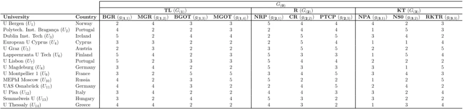
In this section, we show how to apply the proposed methodology to a decision making problem regarding the university ranking. Fourteen European universities, assessed on ten elementary criteria located at the bottom of a hierarchy tree shown in Figure 3, have been extracted from database [1]. Performances of the universities on the considered elementary criteria in the 1-5 scale are shown in Table 1.
Figure 3: Hierarchical structure of criteria considered in the case study
G(0) T L G1 BGR g(1,1) M GR g(1,2) BGOT g(1,3) M GOT g(1,4) R G2 N RP g(2,1) CR g(2,2) P T CP g(2,3) KT G3 N P A g(3,1) N SO g(3,2) RKT R g(3,3)
Table 1: Evaluations of the universities at hand on the considered elementary criteria
G(0)
TL(G(1)) R(G(2)) KT(G(3))
University Country BGR(g(1,1)) MGR(g(1,2)) BGOT(g(1,3)) MGOT(g(1,4)) NRP(g(2,1)) CR(g(2,2)) PTCP(g(2,3)) NPA(g(3,1)) NS0(g(3,2)) RKTR(g(3,3))
U Bergen (U1) Norway 2 4 3 3 5 4 4 4 2 3
Polytech. Inst. Bragan¸ca (U2) Portugal 4 2 2 3 2 4 4 1 5 3
Dublin Inst. Tech (U3) Ireland 5 2 4 4 2 5 5 3 4 2
European U Cyprus (U4) Cyprus 3 3 2 2 2 5 4 1 1 4
U Graz (U5) Austria 2 3 2 2 3 5 5 2 2 5
Lappeenranta U Tech (U6) Finland 5 4 2 3 5 3 3 1 5 4
U Lisbon (U7) Portugal 5 2 3 3 5 4 4 2 2 2
U Magdeburg (U8) Germany 3 4 2 2 5 3 3 3 1 5
U Montpellier 1 (U9) France 3 2 5 5 3 4 5 3 4 3
MEPhI Moscow (U10) Russia 4 2 3 5 5 2 2 1 2 5
UAS Osnabr¨uck (U11) Germany 4 4 3 2 2 4 5 2 4 2
U Pisa (U12) Italy 3 4 2 2 4 4 3 3 2 4
Semmelweis U (U13) Hungary 3 2 4 4 5 3 2 3 2 2
U Thessaly (U14) Greece 4 4 2 2 4 3 2 1 3 4
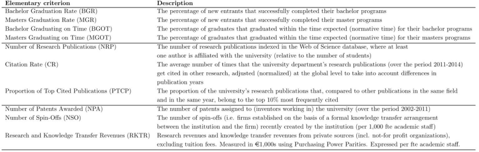
In Table 2, we provide a description of the ten elementary criteria. As one can see from Figure 3, Teaching and Learning (TL), Research (R) and Knowledge Transfer (KT) are macro-criteria. Masters Graduation Rate (MGR), Masters Graduating on Time (MGT), Bachelor Graduation Rate (BGR) and Bachelor Graduating on Time (BGT) are elementary criteria descending from Teaching and Learning; Number of Research Publications (NRP), Citation Rate (CR) and Proportion of Top Cited Publications (PTCP) are elementary criteria desceding from Research, while Number
Table 2: Description of the elementary criteria Elementary criterion Description
Bachelor Graduation Rate (BGR) The percentage of new entrants that successfully completed their bachelor programs Masters Graduation Rate (MGR) The percentage of new entrants that successfully completed their master programs
Bachelor Graduating on Time (BGOT) The percentage of graduates that graduated within the time expected (normative time) for their bachelor programs Masters Graduating on Time (MGOT) The percentage of graduates that graduated within the time expected (normative time) for their masters programs Number of Research Publications (NRP) The number of research publications indexed in the Web of Science database, where at least
one author is affiliated with the university (relative to the number of students)
Citation Rate (CR) The average number of times that the university department’s research publications (over the period 2011-2014) get cited in other research, adjusted (normalized) at the global level to take into account differences in publication years
Proportion of Top Cited Publications (PTCP) The proportion of the university’s research publications that, compared to other publications in the same field and in the same year, belong to the top 10% most frequently cited
Number of Patents Awarded (NPA) The number of patents assigned to (inventors working in) the university (over the period 2002-2011) Number of Spin-Offs (NSO) The number of spin-offs (i.e. firms established on the basis of a formal knowledge transfer arrangement
between the institution and the firm) recently created by the institution (per 1,000 fte academic staff) Research and Knowledge Transfer Revenues (RKTR) Research revenues and knowledge transfer revenues from private sources (incl. not-for profit organizations),
excluding tuition fees. Measured ine1,000s using Purchasing Power Parities. Expressed per fte academic staff.
of Patents Awarded (NPA), Number of Spin-Offs (NSO) and Research and Knowledge Transfer Revenues (RKTR) are all elementary criteria descending from Knowledge Transfer.
Let us suppose that the following information has been provided, as specified in Step 1 of the scheme presented in Section 4:
1.1 The indifference, preference and veto thresholds are equal to 1, 2 and 4 respectively, for all elementary criteria; that is qt= 1, pt = 2 andvt= 4 for all t∈EL.
1.2 The following interactions and antagonistic effects exist:
– CR and PTCP present a mutual-weakening effect,
– NRP and RKTR present a mutual-strengthening effect,
– PTCP presents an antagonistic effect over MGR.
1.3 The imprecise SRF method is applied to the direct subcriteria of each non-elementary criterion as follows:
– with respect to the first level criteria, T Lis less important than KT that, in turn, is less important than R. The number of blank cards inserted between KT and T L belongs to the interval [0,1], while the number of blank cards inserted betweenR andKT belongs to the interval [1,2]; moreover, the ratio between the importance of R and the importance of T L belongs to the interval [2,3],
– considering the macro-criterionT L,BGRis less important thanBGOT and the number of blank cards inserted between them belongs to the interval [0,1]. BGOT is less important than M GR and the number of cards inserted between them belongs to the interval [1,2]. Finally, M GR is less important than M GOT and the number of blank cards inserted between them belongs to the interval [0,1]. The ratio between the importance ofM GOT
and the importance of M GR belongs to the interval [2,3],
– with respect to the macro-criterion R, N RP is less important than P T CP that, in turn, is less important thanCR. The number of blank cards inserted betweenP T CP andN RP
belongs to the interval [0,1], while the number of blank cards inserted between CR and
P T CP belongs to the interval [1,2]. The ratio between the importance of CR and the
importance of N RP belongs to the interval [2,3],
– considering the macro-criterion KT, N P A is less important than N SO that, in turn, is less important thanRKT R. The number of blank cards inserted betweenN SOandN P A
belongs to the interval [1,2], while the number of blank cards inserted between RKT R
and N SO belongs to the interval [0,1]. Moreover, the ratio between the importance of
RKT R and the importance ofN P A belongs to the interval [4,5].
Considering the preference information provided by the DM, we solved the LP problem (15) that gave ε∗ > 0. This means that there exists at least one compatible vector. In order to get robust recommendations, we applied the SMAA methodology on results of the hierarchical ELECTRE III method with interactions, obtained for a sample of compatible vectors. Consequently, for each non-elementary criterion, we computed the preference, indifference and incomparability relations, as well as the indices shown in Section 4. A complete data set of results can be downloaded clicking on the following link: dataMCHPELECTRE.
Table 3: Frequencies of the preference, incomparability and indifference relations between the considered universities at the comprehensive level
(a) Preference
University / University U1 U2 U3 U4 U5 U6 U7 U8 U9 U10 U11 U12 U13 U14
U Bergen (U1) 0 0 0 13.19 0 0 100 0 0 11.24 52.22 0 100 51.07
Polytech. Inst. Bragan¸ca (U2) 87.29 0 0 100 0 0 100 0.29 0 83.66 52.44 0 100 100
Dublin Inst. Tech (U3) 100 99.35 0 100 0 0 100 0.29 0 100 100 14.87 100 100
European U Cyprus (U4) 0 0 0 0 0 0 87.60 0 0 0 14.95 0 45.48 26.15 U Graz (U5) 100 99.51 10.46 100 0 0 100 10.75 0 100 100 24.91 100 100 Lappeenranta U Tech (U6) 100 100 100 100 100 0 100 100 99.79 100 100 100 100 100 U Lisbon (U7) 0 0 0 0 0 0 0 0 0 0 0 0 0.94 0 U Magdeburg (U8) 99.70 89.05 0 100 0 0 100 0 0 73.0 52.22 38.74 100 99.86 U Montpellier 1 (U9) 100 100 99.89 100 99.81 0 100 99.59 0 100 100 99.89 100 100 MEPhI Moscow (U10) 24.39 0 0 0 0 0 100 0 0 0 52.22 0 100 39.84
UAS Osnabr¨uck (U11) 46.62 0 0 0 0 0 100 0 0 42.80 0 0 63.14 47.78
U Pisa (U12) 99.70 84.77 0 100 0 0 100 21.42 0 83.66 52.22 0 100 100 Semmelweis U (U13) 0 0 0 0 0 0 98.32 0 0 0 0 0 0 0 U Thessaly (U14) 19.09 0 0 52.22 0 0 100 0 0 15.61 52.22 0 87.53 0 (b) Incomparability University / University U1 U2 U3 U4 U5 U6 U7 U8 U9 U10 U11 U12 U13 U14 U Bergen (U1) 0 0.29 0 86.80 0 0 0 0.29 0 2.24 0.865 0.29 0 20.88
Polytech. Inst. Bragan¸ca (U2) 0.29 0 0.29 0 0.29 0 0 10.65 0 16.33 47.56 0.35 0 0
Dublin Inst. Tech (U3) 0 0.29 0 0 0 0 0 99.70 0 0 0 85.13 0 0
European U Cyprus (U4) 86.80 0 0 0 0 0 12.39 0 0 100 85.04 0 54.51 21.62 U Graz (U5) 0 0.29 0 0 0 0 0 89.24 0 0 0 75.08 0 0 Lappeenranta U Tech (U6) 0 0 0 0 0 0 0 0 0 0 0 0 0 0 U Lisbon (U7) 0 0 0 12.39 0 0 0 0 0 0 0 0 0 0 U Magdeburg (U8) 0.29 10.65 99.70 0 89.24 0 0 0 0.41 26.93 47.78 0.15 0 0.14 U Montpellier 1 (U9) 0 0 0 0 0 0 0 0.41 0 0 0 0.10 0 0 MEPhI Moscow (U10) 2.24 16.33 0 100 0 0 0 26.93 0 0 0 16.33 0 36.60
UAS Osnabr¨uck (U11) 0.86 47.56 0 85.04 0 0 0 47.78 0 0 0 47.78 0 0
U Pisa (U12) 0.29 0.35 85.13 0 75.08 0 0 0.15 0.10 16.33 47.78 0 0 0 Semmelweis U (U13) 0 0 0 54.51 0 0 0 0 0 0 0 0 0 0 U Thessaly (U14) 20.88 0 0 21.62 0 0 0 0.14 0 36.60 0 0 0 0 (c) Indifference University / University U1 U2 U3 U4 U5 U6 U7 U8 U9 U10 U11 U12 U13 U14 U Bergen (U1) 0 12.42 0 0 0 0 0 0 0 62.12 0.29 0 0 8.96
Polytech. Inst. Bragan¸ca (U2) 12.42 0 0.35 0 0.20 0 0 0 0 0 0 14.87 0 0
Dublin Inst. Tech (U3) 0 0.35 0 0 89.54 0 0 0 0.11 0 0 0 0 0
European U Cyprus (U4) 0 0 0 0 0 0 0 0 0 0 0 0 0 0 U Graz (U5) 0 0.20 89.54 0 0 0 0 0 0.19 0 0 0 0 Lappeenranta U Tech (U6) 0 0 0 0 0 0 0 0 0.21 0 0 0 0 0 U Lisbon (U7) 0 0 0 0 0 0 0 0 0 0 0 0 0.74 0 U Magdeburg (U8) 0 0 0 0 0 0 0 0 0 0 0 39.67 0 0 U Montpellier 1 (U9) 0 0 0.11 0 0.19 0.21 0 0 0 0 0 0 0 0 MEPhI Moscow (U10) 62.12 0 0 0 0 0 0 0 0 0 4.98 0 0 7.94
UAS Osnabr¨uck (U11) 0.29 0 0 0 0 0 0 0 0 4.98 0 0 36.86 0
U Pisa (U12) 0 14.87 0 0 0 0 0 39.67 0 0 0 0 0 0
Semmelweis U (U13) 0 0 0 0 0 0 0.74 0 0 0 36.86 0 0 12.47
U Thessaly (U14) 8.96 0 0 0 0 0 0 0 0 7.94 0 0 12.47 0
When interpreting the results, we will call the universities by their location name. As one can see from Tables 3(a) and 4, Lappeenranta can be seen as the best among the 14 universities since it is globally preferred to all the other universities with a frequency equal to at least 99.79%. It is always
Table 4: Mean number of alternatives that are weakly preferred to each university, and mean number of alternatives to which each university is weakly preferred at the comprehensive level
University M eanUisW P to
0 M eanW P to U0
U Bergen (U1) 4.12 8.61
Polytech. Inst. Bragan¸ca (U2) 6.52 6.01
Dublin Inst. Tech (U3) 9.05 3.00
European U Cyprus (U4) 1.74 7.65 U Graz (U5) 9.36 2.90 Lappeenranta U Tech (U6) 13.00 0.00 U Lisbon (U7) 0.02 12.87 U Magdeburg (U8) 7.92 2.72 U Montpellier 1 (U9) 12.00 1.00 MEPhI Moscow (U10) 3.91 7.85
UAS Osnabr¨uck (U11) 3.42 7.71
U Pisa (U12) 7.96 3.33
Semmelweis U (U13) 1.48 11.47
U Thessaly (U14) 3.56 8.94
weakly preferred to all the other universities, while any university is never weakly preferred to it. More in detail, Lappeenranta is always preferred to all alternatives except Montpellier to which it is preferred with frequency of 99.79%. In the remaining cases (0.21%) Lappeenranta is indifferent to Montpellier. As a third option after Lappeenranta and Montpellier, one could consider Graz since, on average, it is weakly preferred to 9.36 universities and only 2.90 universities are weakly preferred to it. Indeed, Lappeenranta and Montpellier are the only universities that can be preferred to Graz. At the same time, Lisbon can be considered as the worst university at the comprehensive level since it is never preferred to any other university, apart from Semmelweis, but with a very small frequency (0.94%). Moreover, looking at Table 4, one can see that Lisbon is weakly preferred to an average number of 0.02 universities, while 12.87 universities are, in average, weakly preferred to it.
Since many vectors of weights and interaction coefficients are compatible with the preference information provided by the DM, we computed, component by component, their barycenter as their mean value (see Table 5). One can observe that criterion CR is the most important among the elementary criteria, which is concordant with the requirement that its macro-criterion R is the most important at the first level. Moreover, one can observe a great importance obtained by the mutual-strengthening effect between N RP and RKT R, since it is equal to 0.526; this value is taken into account in computing the concordance index for pairs of alternatives at the comprehensive level.
Table 5: Barycenter of all sampled compatible vectors
WT L WR WKT 0.214 0.471 0.315 wBGR wM GR wBGOT wM GOT wN RP wCR wP T CP wN P A wN SO wRKT R wCR−P T CP wN RP−RKT R w ′ M GR−P T CP 0.030 0.062 0.042 0.075 0.098 0.230 0.149 0.037 0.121 0.156 -0.040 0.526 0.018
The recommended partial preorder at comprehensive level obtained for the barycenter values is shown in Figure 4. One can see that the conclusions drawn above on the base of the frequencies of preference, indifference and incomparability are confirmed by the partial preorder obtained with the weights and interaction coefficients equal to their barycenter. Lappeenranta and Montpellier take the first two positions in the ranking, while the third place is taken by Magdeburg, Pisa, Dublin and Graz. In particular, Magdeburg is indifferent to Pisa and Dublin is indifferent to Graz. Lisbon takes the last position, while Semmelweis is at the last but one position.
A similar analysis can be performed for each of the three macro-criteria. Here we shall present the results obtained for the TL macro-criterion.
Looking at Table 6(a) one can conclude that Montpellier is the best among the 14 universities on TL since it is preferred to all the other universities with a frequency equal to at least 70.91%. In
Figure 4: The partial preorder obtained at the comprehensive level by applying the hierarhical ELECTRE III method with interactions for the weights and the interaction coefficients in the barycenter
Bergen Moscow Osnabruck Braganca Thessaly Dublin Graz Cyprus Lappeenranta Montpellier Lisbon Magdeburg Pisa Semmelweis
particular, Montpellier is preferred to Dublin, Lappeenranta, Osnabruck and Thessaly with the same frequency (70.91%) and only Dublin and Lappeenranta can be preferred to Montpellier. As to the second best university on TL, according to the results shown in Table 7, this is one of Lappeenranta and Dublin. Indeed, on the one hand, they are weakly preferred to an average of 10.31 and 9.61 universities, respectively, and on the other hand, an average number of only 1.15, 1.84 universities is weakly preferred to them, respectively. Comparing these two universities pairwise one can observe that Dublin is preferred to Lappeenranta with a frequency of 42.92%, while the opposite is true with a frequency of 29.08%. In the remaining 27.99% of the cases, the two universities are incomparable. Looking at the worst university on TL, the choice goes to Bragan¸ca since it can be preferred only to Graz, while all the 13 universities are preferred to it with a frequency equal to at least 70.91%.
Regarding the other universities, some indifferences and incomparabiliries can be observed (see Tables 6(c) and 6(b)). For example, Graz and Cyprus are indifferent in 70.91% of the cases, while Moscow and Thessaly are incomparable with the same frequency.
The final partial preorder obtained for T Land the barycenter values is show in Figure 5.
Again, the partial preorder shown in Figure 5 confirms the indications coming from the frequencies of preference, incomparability and indifference, as well as from the average number of universities being weakly preferred to each university and from the mean number of universities to which each university is weakly preferred. Indeed, Montpellier is the best university on T L, followed by Dublin and Moscow. The last position is taken by Bragan¸ca, while the last but one by Lisbon.
For the sake of completeness we show in Figures 6(a) and 6(b) the partial preorders obtained for the macro-criteriaRandKT obtained with the weights and interaction coefficients in the barycenter.
Table 6: Frequencies of the preference, incomparability and indifference relations between the considered universities with respect to subcriterion T L
(a) Preference
University / University U1 U2 U3 U4 U5 U6 U7 U8 U9 U10 U11 U12 U13 U14
U Bergen (U1) 0 70.91 27.99 100 100 0.13 70.91 27.99 0 20.59 27.99 27.99 27.99 27.99
Polytech. Inst. Bragan¸ca (U2) 0 0 0 0 29.08 0 0 0 0 0 0 0 0 0
Dublin Inst. Tech (U3) 72 100 0 100 100 42.92 100 72 29.08 29.08 72 72 72 72
European U Cyprus (U4) 0 70.91 0 0 29.08 0 70.91 0 0 0 0 0 0 0 U Graz (U5) 0 70.91 0 0 0 0 70.91 0 0 0 0 0 0 0 Lappeenranta U Tech (U6) 72 100 29.08 100 100 0 100 99.86 29.08 29.08 99.86 99.86 72 99.86 U Lisbon (U7) 0 100 0 29.08 29.08 0 0 0 0 0 0 0 29.08 0 U Magdeburg (U8) 29.08 100 0 100 100 0 70.91 0 0 0 0 0 0 0 U Montpellier 1 (U9) 100 100 70.91 100 100 70.91 100 100 0 100 70.91 100 100 70.91 MEPhI Moscow (U10) 29.08 100 27.99 100 100 0 100 29.08 0 0 0 29.08 100 0
UAS Osnabr¨uck (U11) 72 100 0 100 100 0 100 72 0 29.08 0 72 29.08 72
U Pisa (U12) 29.08 100 0 100 100 0 70.91 0 0 0 0 0 0 0 Semmelweis U (U13) 0 100 0 100 100 0 70.91 0 0 0 0 0 0 0 U Thessaly (U14) 29.08 100 0 100 100 0 100 72 0 29.08 0 72 29.08 0 (b) Incomparability University / University U1 U2 U3 U4 U5 U6 U7 U8 U9 U10 U11 U12 U13 U14 U Bergen (U1) 0 29.08 0 0 0 27.85 29.08 42.92 0 50.32 0 42.92 72 42.92
Polytech. Inst. Bragan¸ca (U2) 29.08 0 0 29.08 0 0 0 0 0 0 0 0 0 0
Dublin Inst. Tech (U3) 0 0 0 0 0 27.99 0 27.99 0 42.92 27.99 27.99 0 27.99
European U Cyprus (U4) 0 29.08 0 0 0 0 0 0 0 0 0 0 0 0 U Graz (U5) 0 0 0 0 0 0 0 0 0 0 0 0 0 0 Lappeenranta U Tech (U6) 27.85 0 27.99 0 0 0 0 0 0 70.91 0 0 27.99 0 U Lisbon (U7) 29.08 0 0 0 0 0 0 29.08 0 0 0 29.08 0 0 U Magdeburg (U8) 42.92 0 27.99 0 0 0 29.08 0 0 70.91 0 0 100 0 U Montpellier 1 (U9) 0 0 0 0 0 0 0 0 0 0 29.08 0 0 29.08 MEPhI Moscow (U10) 50.32 0 42.92 0 0 70.91 0 70.91 0 0 70.91 70.91 0 70.91
UAS Osnabr¨uck (U11) 0 0 27.99 0 0 0 0 0 29.08 70.91 0 0 70.91 0
U Pisa (U12) 42.92 0 27.99 0 0 0 29.08 0 0 70.91 0 0 100 0 Semmelweis U (U13) 72 0 0 0 0 27.99 0 100 0 0 70.91 100 0 70.91 U Thessaly (U14) 42.92 0 27.99 0 0 0 0 0 29.08 70.91 0 0 70.91 0 (c) Indifference University / University U1 U2 U3 U4 U5 U6 U7 U8 U9 U10 U11 U12 U13 U14 U Bergen (U1) 0 0 0 0 0 0 0 0 0 0 0 0 0 0
Polytech. Inst. Bragan¸ca (U2) 0 0 0 0 0 0 0 0 0 0 0 0 0 0
Dublin Inst. Tech (U3) 0 0 0 0 0 0 0 0 0 0 0 0 27.99 0
European U Cyprus (U4) 0 0 0 0 70.91 0 0 0 0 0 0 0 0 0 U Graz (U5) 0 0 0 70.91 0 0 0 0 0 0 0 0 0 0 Lappeenranta U Tech (U6) 0 0 0 0 0 0 0 0.13 0 0 0.13 0.13 0 0.13 U Lisbon (U7) 0 0 0 0 0 0 0 0 0 0 0 0 0 0 U Magdeburg (U8) 0 0 0 0 0 0.13 0 0 0 0 27.99 100 0 27.99 U Montpellier 1 (U9) 0 0 0 0 0 0 0 0 0 0 0 0 0 0 MEPhI Moscow (U10) 0 0 0 0 0 0 0 0 0 0 0 0 0 0
UAS Osnabr¨uck (U11) 0 0 0 0 0 0.13 0 27.99 0 0 0 27.99 0 27.99
U Pisa (U12) 0 0 0 0 0 0.13 0 100 0 0 27.99 0 0 27.99
Semmelweis U (U13) 0 0 27.99 0 0 0 0 0 0 0 0 0 0 0
U Thessaly (U14) 0 0 0 0 0 0.13 0 27.99 0 0 27.99 27.99 0 0
Table 7: Mean number of alternatives that are weakly preferred to each university, and mean number of alternatives to which each university is weakly preferred with respect to subcriterionT L
University M eanUisW Pto
T L M eanW PT L toU
U Bergen (U1) 5.31 4.32
Polytech. Inst. Bragan¸ca (U2) 0.29 12.13
Dublin Inst. Tech (U3) 9.61 1.84
European U Cyprus (U4) 2.42 11.00 U Graz (U5) 2.13 11.58 Lappeenranta U Tech (U6) 10.31 1.15 U Lisbon (U7) 1.87 10.25 U Magdeburg (U8) 5.56 6.29 U Montpellier 1 (U9) 11.84 0.58 MEPhI Moscow (U10) 6.15 2.37
UAS Osnabr¨uck (U11) 8.30 3.55
U Pisa (U12) 5.56 6.29
Semmelweis U (U13) 3.99 4.87
Figure 5: The partial preorder obtained onT L by applying the hierarhical ELECTRE III method with interactions for the weights and the interaction coefficients in the barycenter
Bergen Cyprus Graz Braganca Dublin Lappeenranta Lisbon Osnabruck Semmelweis Magdeburg Pisa Montpellier Moscow Thessaly
• with respect to R, Bergen and Lisbon are equally the best and they are followed by Graz and Montpellier. Looking at the tail of the ranking, Moscow and Thessaly take the last two positions in this order. Some incomparabilities exist such that one between Bragan¸ca and Semmelweis or that one between Cyprus and Osnabr¨uck,
• with respect to KT, Lappeenranta is the best among the considered universities, followed by Bragan¸ca and Montpellier. Looking at the tail of the ranking, Lisbon and Semmelweis are equally the worst, while Bergen takes the last but one position.
As underlined in point 5.3 of the scheme presented in the previous section, let us observe that when applying the ELECTRE III method with interactions, we obtained different final partial preorders at comprehensive level as well as at partial level even if we have shown here only the final partial preoders obtained considering the barycenter of the sampled weights and interaction coefficients. In particular, we obtained 39 partial preorders at comprehensive level, 5 partial preorders on Teaching and Learning, and 1 partial preorder only on Research and Knowledge Transfer, being therefore the two partial preorders shown in Figures 6(a) and 6(b), respectively. The frequencies of the obtained partial preorders as well as the barycenter of the weights for which the same partial preorders are obtained can be downloaded clicking on the following link: dataMCHPELECTRE.
To conclude this section, we would like to underline the usefulness of taking into account the MCHP in the decision problem at hand and, in general, in all decision problems involving hierarchical criteria. Let us consider universities of Moscow and Osnabr¨uck. Looking at Table 1, one can observe that the two universities do not dominate each other at any of the three considered macro-criteria. Consequently, looking only at the performances of the universities on the elementary criteria nothing
Bergen Lisbon Graz Montpellier Lappeenranta Magdeburg Braganca Dublin Cyprus Osnabruck Moscow Pisa Thessaly Semmelweis (a) Research Bergen Lisbon Semmelweis Braganca Montpellier Thessaly Dublin Magdeburg Osnabruck Pisa Cyprus Graz Moscow Lappeenranta (b) Knowledge Transfer
Figure 6: The partial preorders obtained on the macro-criteriaRandKT by applying the proposed methodology for the weights and interaction coefficients in the barycenter