Gauss and Poisson approximation: applications to CDO
tranches pricing
Nicole El Karoui, Ying Jiao, David Kurtz
To cite this version:
Nicole El Karoui, Ying Jiao, David Kurtz. Gauss and Poisson approximation: applications to CDO tranches pricing. 2008. <hal-00324208>
HAL Id: hal-00324208
https://hal.archives-ouvertes.fr/hal-00324208
Submitted on 24 Sep 2008
HAL is a multi-disciplinary open access
archive for the deposit and dissemination of sci-entific research documents, whether they are
pub-lished or not. The documents may come from
teaching and research institutions in France or abroad, or from public or private research centers.
L’archive ouverte pluridisciplinaire HAL, est
destin´ee au d´epˆot et `a la diffusion de documents
scientifiques de niveau recherche, publi´es ou non,
´emanant des ´etablissements d’enseignement et de
recherche fran¸cais ou ´etrangers, des laboratoires
Gauss and Poisson Approximation: Applications to
CDOs Tranche Pricing
September 22, 2008
Nicole El Karoui CMAP Ecole Polytechnique Palaiseau 91128 Cedex France [email protected]
Ying Jiao
Laboratoire de Probabilit´es et Mod`eles Al´eatoires Universit´e Paris VII
[email protected] David Kurtz
BlueCrest Capital Management Limited
40 Grosvenor Place, London, SW1X 7AW, United Kingdom [email protected]
Abstract
This article describes a new numerical method, based on Stein’s method and zero bias transformation, to compute CDO tranche prices. We propose first order correction terms for both Gauss and Poisson approximations and the approximation errors are discussed. We then combine the two approximations to price CDOs tranches in the condi-tionally independent framework using a realistic local correlation struc-ture. Numerical tests show that the method provides robust results with a very low computational burden.
Acknowledgement: this work is partially supported by La Fondation du Risque. We are also grateful to the referees for very valuable comments and suggestions.
1
Introduction
In the growing credit derivatives market, correlation products like CDO play a major role. On one hand, CDO enables financial institutions to transfer efficiently the credit risk of a pool of names in a global way. On the other hand, the investors can choose to invest on different tranches according to their risk aversion.
The key term to value a CDO tranche is the law of the cumulative loss of the underlying portfolio lt=Pni=1 NNi(1−Ri)I{τi≤t}, where Ni, Ri, τi are
respectively the notional value, the recovery rate and the default time of name i and N the total portfolio notional defined by N = Pni=1Ni. The critical issue for CDO pricing is to compute the valueE[(lt−k)+], which is
a call function on the cumulative loss.
The standard market model for the default correlation is the factor model ([1],[14]), where the default events are supposed to be conditionally indepen-dent given a common factorU. In the literature, there exist approximation methods for the conditional distribution and then integrating (see [11], [18]). In fact, conditional on U, the cumulative losslt can be written as a sum of independent random variables. Using the central limit theorem, it is then natural to apply Gauss or Poisson approximation to compute the conditional cumulative losses distribution.
The binomial-normal approximation has been studied in various financial problems. It is well known that the price of an European option calculated in the binomial tree model converges to its Black-Scholes price when the discretization number tends towards infinity. In particular, Diener and Di-ener [9] have proved that in this symmetric binomial case, the convergence speed is of orderO(1/n). In the credit analysis, Vasicek [24] has introduced the normal approximation to a homogeneous portfolio of loans. As the de-fault probabilities are in general small and not equal to 1/2, the convergence speed is of orderO(1/√n) in the general case.
Other numerical methods such as the saddle-point method ([16], [17], [2]) have been proposed. The saddle-point method consists in expanding around the saddle point to approximate a function of the cumulant generating func-tion of condifunc-tional losses. It coincides with the normal approximafunc-tion when choosing some particular point. In the inhomogeneous case, it is rather costly to find the saddle-point numerically. In addition, although proven efficient by empirical tests, there is no discussion of the error estimations in aforementioned papers.
The Poisson approximation, less discussed in the financial context, is known to be robust for small probabilities in the approximation of binomial laws. One usually asserts that the normal approximation remains robust when np ≥ 10. If np is small, the binomial law approaches a Poisson law. In our case, the size of the portfolio is fixed for a standard synthetic CDO tranche andn≈125. On the other hand, the conditional default probability
p(U) varies in the interval (0,1) according to its explicit form with respect to the factorU. Hence we may encounter both cases and it is mandatory to study the convergence speed since nis finite.
Stein’s method is an efficient tool to estimate the approximation errors in the limit theorem problems. In this paper, we provide, by combining Stein’s method and the zero bias transformation, first-order correction terms for both Gauss and Poisson approximations. Error estimations of corrected ap-proximations are obtained. These first order apap-proximations can be applied to conditional distributions in the general factor framework and the CDOs tranches prices can then be obtained by integration across the common fac-tors.
Thanks to the simple form of the formulas, we reduce largely the com-putational burden for CDOs prices. In addition, the summand variables are not required to be identically distributed, which corresponds to inhomoge-neous CDO tranches. We present in Section 2 the theoretical results and Section 3 and 4 are devoted to numerical tests on CDOs. Section 5 contains the conclusion and perspective remarks. We gather at last some technical results and proofs in Appendix.
2
First-Order Correction of Conditional Losses
2.1 First-order Gaussian correction
In the classical binomial-normal approximation, the expectation of functions of conditional losses can be calculated using a Gaussian expectation. More precisely, the expectation E[h(W)] where W is the sum of conditionally
in-dependent individual loss variables can be approximated by ΦσW(h) defined
by ΦσW(h) = √ 1 2πσW Z ∞ −∞ h(u) exp− u 2 2σ2W du (1)
whereσW is the standard deviation ofW. The error of this zero-order ap-proximation is of orderO(1/√n) by the well-known Berry-Esseen inequality using the Wasserstein distance ([19], [8]) except in the symmetric case.
We shall improve the approximation quality by finding a correction term such that the corrected error is of order O(1/n) even in the asymmetric case. Some regularity conditions are required on the considered functionh. Notably, the call function, not possessing second order derivative, is difficult to analyze. In the following theorem, we give the corrector term for regular enough functions. The explicit error bound and the proof can be found in Appendix 6.2.1.
Theorem 2.1 Let X1, . . . , Xn be independent mean zero random variables
and σ2
W = Var[W]. For any function h such that kh′′k exists, the normal
approximationΦσW(h) of E[h(W)] has corrector
Ch = µ(3) 2σ4 W ΦσW x2 3σ2 W −1xh(x) (2)
where µ(3)=Pni=1E[Xi3]. The corrected approximation error is bounded by E[h(W)]−Φσ W(h)−Ch ≤α h, X1, . . . , Xn where α h, X1, . . . , Xn
, precised later in (22), depends on h′′ and on the moments of Xi up to the fourth order.
The corrector is written as the product of two terms: the first one de-pends on the moments ofXi up to the third order and the second one is a normal expectation of some polynomial function multiplyingh. Both terms are simple to calculate, even in the inhomogeneous case.
To adapt to the definition of the zero bias transformation, which will be introduced in Section 6.1.1, and also to obtain a simple representation of the corrector, the variablesXi’s are set to be of zero expectation in Theorem 2.1. This condition requires a normalization step when applying the theorem to conditional losses. A useful example concerns the centered Bernoulli random variables which take two real values and have zero expectation.
Note that the moments of Xi play an important role here. In the sym-metric case we haveµ(3) = 0 and as a consequenceCh = 0 for any function h. Therefore, Ch can be viewed as an asymmetric corrector in the sense that, after correction, the approximation realizes the same error order as in the symmetric case.
To specify the convergence order of the corrector, let us consider the normalization of an homogeneous case whereXi are i.i.d. random variables whose moments may depend on n. Notice that
ΦσW x2 3σ2 W −1xh(x) =σWΦ1 x2 3 −1 xh(σWx) .
To ensure that the above expectation term is of constant order, we often suppose that the variance of W is finite and does not depend on n. In this case, we have µ(3) ∼ O(1/√n) and the corrector Ch is also of order O(1/√n). Consider now the percentage default indicator variableI{τi≤t}/n,
whose conditional variance given the common factor is equal top(1−p)/n2 wherep is the conditional default probability of the ith credit, identical for all in the homogeneous case and depends on the common factor. Hence, we shall fix p to be zero order and let Xi = (I{τi≤t}−p)/
√
n. Then σW is of constant order as stated above. Finally, for the percentage conditional loss, the corrector is of orderO(1/n) because of the remaining coefficient 1/√n.
The Xi’s are not required to have the same distribution: we can handle easily different recovery rates (as long as they are independent r.v.) by com-puting the moments of the product variables (1−Ri)I{τi≤t}. The corrector
depends only on the moments ofRiup to the third order. Note however that the dispersion of the recovery rates alongside the dispersion of the notional values can have an impact on the order of the corrector.
We now concentrate on the call function h(x) = (x−k)+. The Gauss
approximation corrector is given in this case by Ch =
µ(3) 6σ2
W
kφσW(k) (3)
where φσ is the density function of the distribution N(0, σ2). When the strikek= 0, the correctorCh = 0. On the other hand, the functionkexp −
k2
2σ2 W
reaches its maximum and minimum values whenk=σW andk=−σW respectively, and then tends to zero quickly.
The numerical computation of this corrector is extremely simple since there is no need to take expectation. Observe however that the call func-tion is a Lipschitz funcfunc-tion with h′(x) = I
{x>k} and h′′ exists only in the
distribution sense. Therefore, we can not apply directly Theorem 2.1 and the error estimation deserves a more subtle analysis. The main tool we used to establish the error estimation for the call function is a concentration in-equality of Chen and Shao [7]. For detailed proof, interested reader may refer to El Karoui and Jiao [10].
We shall point out that the regularity of the function h is essential in the above result. For more regular functions, we can establish correction terms of corresponding order. However, for the call function, the second order correction can not bring further improvement to the approximation results in general.
2.2 First-order Poisson correction
Following the same idea, if V is a random variable taking non-negative integers, then we may approximateE[h(V)] by a Poisson function
PλV(h) = n X l=0 λl V l! e −λVh(l).
The Poisson approximation is robust under some conditions, for example, when V ∼ B(n, p) and np < 10. We shall improve the Poisson approxi-mation by presenting a corrector term as above. We remark that due to the property that a Poisson distributed random variable takes non-negative integer values, the variablesYi’s in Theorem 2.2 are discrete integer random variables. Similar as in the Gaussian case, the proof of the following theorem is postponed to Appendix 6.2.2.
Theorem 2.2 Let Y1, . . . , Yn be independent random variables taking
non-negative integer values such that E[Yi3] (i = 1, . . . , n) exist. Let V =
Y1 +· · ·+Yn with expectation and variance λV = E[V] and σV2 = Var[V].
Then, for any bounded functionh defined onN+, the Poisson approximation
PλV(h) of E[h(V)]has corrector ChP = σ 2 V −λV 2 PλV(∆ 2h) (4)
where Pλ(h) =E[h(Λ)] with Λ ∼ P(λ) and ∆h(x) = h(x+ 1)−h(x). The
corrected approximation error is bounded by
E[h(V)]− Pλ V(h)−C P h ≤β(h, Y1, . . . , Yn)
where β(h, Y1, . . . , Yn), precised later in (30), depends on h and on the
mo-ments of Yi up to the third order. The Poisson corrector CP
h is of similar form with the Gaussian one and contains two terms as well: one term depends on the moments ofYi and the other is a Poisson expectation.
Since Yi’s are N+-valued random variables, they can represent directly
the default indicatorsI{τi≤t}. This fact limits however the recovery rates to
be identical or proportional for all credits. We now consider the order of the corrector. Suppose thatλV does not depend on nto ensure thatPλV(∆
2h)
is of constant order. Then in the homogeneous case, the conditional default probability p ∼ O(1/n). For the percentage conditional losses, as in the Gaussian case, the corrector is of order O(1/n) with the coefficient 1/n.
Consider the call function h(x) = (x−k)+ wherekis a positive integer.
Since ∆2h(x) =I{x=k−1}, its Poisson approximation corrector is given by
ChP = σ 2 V −λV 2(k−1)!e −λVλk−1 V . (5) The corrector vanishes when the expectation and the variance of the sum variable V are equal. The difficulty here is that the call function is not bounded. However, we can prove that Theorem 2.2 holds for any function of linear increasing speed (see [10]).
2.3 Other approximation methods
There exist other approximation methods, notably the Gram-Charlier ex-pansions and the saddle-point method, to calculate the portfolio products prices. Both methods can be applied to conditional losses. We use the notations as in Section 2.1.
The Gram-Charlier expansion has been used to approximate the bond prices [22] through expansion of the density function of a given random vari-able by using the Gaussian density and cumulants. We shall note that in the
expectation term (2), the polynomial function multiplied byh corresponds to the first order Gram-Charlier expansion. However, the higher order terms obtained by our method are different. For comparison of Gram-Charlier and other expansions (Edgeworth expansion for example), one can consult [22]. The saddle-point method consists of writing the considered expectation function as an integral which contains the cumulant generating function
K(ξ) = lnE[exp(ξW)]. For example,
E[(W −k)+] = lim A→+∞ 1 2πi Z c+iA c−iA exp(K(ξ)−ξk) ξ2 dξ (6)
wherecis a real number. In general, the expansion of the integrand function is made around its critical point — the saddle point, where the integrand function decreases rapidly and hence is most dense. By choosing some par-ticular point to make the expansion, the saddle point method may coincide with the classical Gauss approximation. In [2], the saddle point is chosen such thatK′(ξ
0) =k and the authors propose to approximate E[(W −k)+]
by expansion formulas of increasing precision orders.
It is important to note that in the saddle-point method, the first step is to obtain the value of the saddle point ξ0, which is equivalent to find the
solution of the equationK′(ξ) =k. In the homogeneous case whereXi’s are
i.i.d. random variables given byXi =γ(I{τi≤t}−p) withγ = 1/
p
np(1−p), we have the explicit solution
ξ0= p np(1−p) lnpnpp(1−p) +k(1−p) np(1−p)−kp .
However, in the inhomogeneous case, it consists in solving the equation numerically, which can be rather tedious. In addition, although empirically proved to be efficient, there is no discussions on convergence speed for the above two methods.
3
Numerical Tests on Conditional Losses
Before going further on applications to the CDOs pricing, we would like in this section to perform some basic testings of the preceding formulas. In the sequel, we consider the call value E[(l−k)+] wherel =n−1Pni=1(1−
Ri)ξi and the ξi’s are independent Bernoulli random variable with success probability equal to pi.
3.1 Validity Domain of the Approximations
We begin by testing the accuracy of the corrected Gauss and Poisson ap-proximations for different values ofnp=Pni=1piin the caseRi= 0,n= 100 and for different values of k. The benchmark value is obtained through the
np=1 -0.030% -0.020% -0.010% 0.000% 0.010% 0.020% 0.030% 0.040% 0% 100% 200% 300%
Error Gauss Error Poisson
np=5 -0.010% -0.005% 0.000% 0.005% 0.010% 0.015% 0.020% 0% 100% 200% 300%
Error Gauss Error Poisson
np=10 -0.008% -0.006% -0.004% -0.002% 0.000% 0.002% 0.004% 0.006% 0.008% 0.010% 0.012% 0% 100% 200% 300%
Error Gauss Error Poisson
np=20 -0.008% -0.006% -0.004% -0.002% 0.000% 0.002% 0.004% 0.006% 0.008% 0.010% 0.012% 0% 100% 200% 300%
Error Gauss Error Poisson
Figure 1: Gauss and Poisson approximation errors for various values of np as a function of the strike over the expected loss.
recursive methodology well known by the practitioners ([15], [5]) which com-putes the loss distribution by reducing the portfolio size by one name at each recursive step.
In Figure 1 we plot the differences between the corrected Gauss ap-proximation and the benchmark (Error Gauss) and the corrected Poisson approximation and the benchmark (Error Poisson) for different values of np as a function of the call strike over the expected loss. Note that when the tranche strike equals the expected loss, the normalized strike value in the Gaussian case equals zero due to the centered random variables, which means that the correction vanishes. We also observe that the Gaussian error is maximal around this point.
We observe on these graphs that the Poisson approximation outperforms the gaussian one for approximatelynp <15. On the contrary, for large value of np, the Gauss approximation is the best one. Because of the correction, the threshold between the Gauss-Poisson approximation is higher than the classical one np ≈ 10. In addition, the threshold may be chosen rather flexibly around 15. Combining the two approximations, the minimal error
of the two approximations is relatively larger in the overlapping area when np is around 15. However, we obtain satisfactory results even in this case. In all the graphs presented, the error of the mixed approximation is inferior than 1 bp.
Our tests are made with inhomogeneouspi’s obtained as pi=pexp(σWi−0.5σ2)
(log-normal random variable with expectationp and volatilityσ) whereWi is a family of independent standard normal random variables and values of σ ranging from 0% to 100%. Qualitatively, the results were not affected by the heterogeneity of thepi’s.
Observe that there is oscillation in the Gauss approximation error, while the Poisson error is relatively smooth. This phenomenon is related to the discretisation impact of discrete distributions.
As far as a unitary computation is concerned (one call price), the Gauss and Poisson approximation perform much better than the recursive method-ology: we estimate that these methodologies are 200 times faster. To be fair with the recursive methodology one has to recall that by using it we obtain not only a given call price but the whole loss distribution with which we can obtain several strikes values at the same time. In that case, our approxima-tions outperform the recursive methodology by a factor≥30 with six strike values (3%, 6%, 9%, 12%, 15%, 22%).
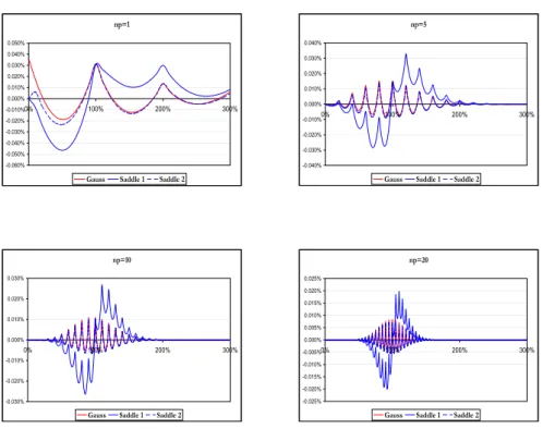
3.2 Saddle-point method and Gauss approximation
We now compare numerically the saddle-point method in [2] and the Gauss approximation for different values ofnp. In Figure 2 are presented the errors of the first order Gauss approximation, and of the first and the second saddle point approximations, as a function of the call strike over the expected loss. The errors of the second order saddle-point method are comparable with the Gauss approximation in all tests. Note that the saddle-point method has also been discussed for non-normal distributions (see [25]) and deserves further studies for CDOs computations.
The tests are applied to the homogeneous case for constant values of p and the calculation times for the saddle point method have outperformed the first order Gauss approximation. However this is no longer true in the inhomogeneous case.
3.3 Stochastic Recovery Rate - Gaussian case
We then consider the case of stochastic recovery rate and check the validity of the Gauss approximation in this case. Following the standard in the industry (Moody’s assumption), we will model theRi’s as independent beta
np=1 -0.060% -0.050% -0.040% -0.030% -0.020% -0.010% 0.000% 0.010% 0.020% 0.030% 0.040% 0.050% 0% 100% 200% 300%
Gauss Saddle 1 Saddle 2
np=5 -0.040% -0.030% -0.020% -0.010% 0.000% 0.010% 0.020% 0.030% 0.040% 0% 100% 200% 300%
Gauss Saddle 1 Saddle 2
np=10 -0.030% -0.020% -0.010% 0.000% 0.010% 0.020% 0.030% 0% 100% 200% 300%
Gauss Saddle 1 Saddle 2
np=20 -0.025% -0.020% -0.015% -0.010% -0.005% 0.000% 0.005% 0.010% 0.015% 0.020% 0.025% 0% 100% 200% 300%
Gauss Saddle 1 Saddle 2
Figure 2: Gauss and Saddle-point methods approximation errors for various values ofnp as a function of the strike over the expected loss.
random variables with expectation 50% and standard deviation 26%. In addition,Ri is independent of ξi.
An application of Theorem 2.1 is used so that the first order corrector term takes into account the first three moments of the random variablesRi. To describe the obtained result, let us first introduce some notation. Let µRi, σ
2
Ri andγ
3
Ri be the first three centered moments of the random variable
Ri, namely µRi =ERi, σ 2 Ri =E(Ri−µRi) 2, γ3 Ri =E(Ri−µRi) 3.
We also define Xi = n−1(1−Ri)ξi −µi where µi = n−1(1−µRi)pi and
pi =Eξi. LetW be Pni=1Xi. We have σW2 := Var(W) = n X i=1 σ2Xi where σ2Xi = pi n2 h σR2i+ (1−pi)(1−µRi) 2i.
Finally, if ˜k=k−Pni=1µi, we have the following approximation
E(l−˜k) +≃ΦσW(· −k)++ 1 6 1 σW2 n X i=1 EXi3]˜kφσ W(˜k) where EXi3= pi n3 h (1−µRi) 3 1 −pi)(1−2pi) + 3(1−pi)(1−µRi)σ 2 Ri−γ 3 Ri i . The benchmark is obtained using standard Monte Carlo integration with 106 simulations. In Figure 3, we display the difference between the approx-imated call price and the benchmark as a function of the strike normalized by the expected loss. We also consider the lower and upper 95% confidence interval for the Monte Carlo results. As in the standard case, one observes that the greater the value ofnpthe better the approximation. Furthermore, the stochastic recovery brings a smoothing effect as the conditional loss no longer follows a binomial law.
The Poisson approximation, due to constraint of integer valued random variables, can not be used directly in the stochastic recovery rates case. We try however to take the mean value of Ri’s as the uniform recovery rate without improving the results except for very low strike (equal to a few bp).
4
Application to CDOs portfolios
In this section, we want to test on real life examples the approaches devel-oped in the preceding sections. We will work in the conditionally indepen-dent framework. In other words, we will assume that conditionally on a risk factorU the default indicators of the names in the considered pool are independent.
np=1 -0.01% -0.01% 0.00% 0.01% 0.01% 0.02% 0.02% 0.03% 0.03% 0% 1% 2% 3% 4% 5%
Lower MC Bound Gauss Error Upper MC Bound
np=5 -0.0050% -0.0040% -0.0030% -0.0020% -0.0010% 0.0000% 0.0010% 0.0020% 0.0030% 0.0040% 0% 1% 2% 3% 4% 5% 6% 7% 8% 9% 10%
Lower MC Bound Gauss Error Upper MC Bound
np=10 -0.0040% -0.0030% -0.0020% -0.0010% 0.0000% 0.0010% 0.0020% 0.0030% 0.0040% 0% 2% 4% 6% 8% 10% 12% 14%
Lower MC Bound Gauss Error Upper MC Bound
np=20 -0.0050% -0.0040% -0.0030% -0.0020% -0.0010% 0.0000% 0.0010% 0.0020% 0.0030% 0.0040% 0.0050% 0% 2% 4% 6% 8% 10% 12% 14% 16% 18% 20%
Lower MC Bound Gauss Error Upper MC Bound
Figure 3: Gauss approximation error in the stochastic recovery case for various values of np as a function of the strike. Comparison with Monte Carlo 1,000,000 simulations. 95% confidence interval.
Let us introduce the notation. We consider a portfolio of n issuers and we will assume for the sake of simplicity that the weight of each firm in the portfolio is the same is equal to 1/n and that the recovery rate for each of these credits is constant and equal to a fixed value R fixed at 40%. The percentage loss on the pool for a given time horizontis defined as
lt= 1−R n n X i=1 I{τi≤t}.
The first step to value properly a CDO is to define the correlation between the default events.
4.1 Modelling the Correlation
Practically, one defines a correlation structure using the conditionally inde-pendent framework. In a nutshell, this tantamounts to postulate the exis-tence of a random variableU (that we may assume uniformly distributed on (0, 1) without loss of generality) such that, conditionally on U, the events Ei ={τi ≤t} are independent. To completely specify a correlation model, one has to choose a function F such that
Z 1
0
F(p, u)du=p, 0≤F ≤1. Ifpi =P[Ei], one simply interpretsF(pi, u) as P[Ei|U =u].
The standard Gaussian copula case with correlationρcorresponds to the functionF defined by F(p, u) =N N−1(p)−√ρN−1(u) √ 1−ρ
where N(x) is the distribution function of N(0,1). The main drawback of the Gaussian correlation approach is the fact that one cannot find a unique model parameter ρ to price all the observed market tranches on a given basket. This phenomenon is referred to as correlation skew by the market practitioners.
In our tests, we will apply a more general approach ([23], [4]) in which the functionF is defined in a non parametric way in order to retrieve the observed market prices of tranches. This function has been calibrated on market prices of the five year tranches 0%-3%, 3%-6%, 6%-9%, 9%-12%, 12%-15% and 15%-22% on a bespoke basket whose prices are observed on a monthly basis.
4.2 CDOs Payoff
Let us describe the payoff of a CDO. Let a and b be the attachment and detachment point expressed in percentage and let
be the loss on the tranche [a, b]. The outstanding notional on the tranche is defined as ca,bt = 1− l a,b t b−a
whereas the tranche survival probability is given byq(a, b, t) =E[ca,bt ]
com-puted under any risk-neutral probability.
The value of the default leg and the premium leg of a continuously com-pounded CDO of maturityT are given respectively by the following formu-las:
Default Leg =−(b−a)
Z T
0
B(0, t)q(a, b,dt), Premium Leg = Spread×(b−a)
Z T
0
B(0, t)q(a, b, t)dt
where B(0, t) is the value at time 0 of a zero coupon maturing at time t. We here assume that the interest rates are deterministic. Thanks to the integration by part formula, the fair spread is then computed as follow
Fair Spread = 1−B(0, T)q(a, b, T) + Z T 0 q(a, b, t)B(0,dt) Z T 0 B(0, t)q(a, b, t)dt . (7)
To compute the value of the preceding integrals, we begin by approxi-mating the logarithm of the functionsqandBby linear splines with monthly pillars forq (adding the one week point for short term precision) and weekly pillars forB. The integrals are then computed using time step of length one week. Performing these operations boils down to compute call prices value of the formC(t, k) =E[(lt−k)+].
4.3 Gauss Approximation
We describe in this subsection the Gauss approximation that can be used to compute in an efficient way the call prices in any conditionally independent model.
Let µi and σi be respectively the expectation and standard deviation of the random variable χi = n−1(1−R)I{τi≤t}. Let Xi = χi −µi and
W =Pni=1Xi, so that the expectation and standard deviation of the random variable W are 0 and σW := qPin=1σ2i respectively. Let also pi be the default probability of issueri. We want to calculate
where ˜k =k−Pni=1µi. Remark that pi and k are in fact all functions of the common factor.
Assuming that the random variable Xi’s are mutually independent, the result of Theorem 2.1 may be stated in the following way
C(t, k)≃ Z +∞ −∞ dx φσW(x)(x−˜k)++ 1 6 1 σ2 W n X i=1 E[Xi3]˜kφσW(˜k) (8) where E[Xi3] = (1−R) 3
n3 pi(1−pi)(1−2pi). The first term on the right-hand
side of (8) is the Gauss approximation that can be computed in closed form thanks to Bachelier formula whereas the second term is a correction term that account for the non-normality of the loss distribution.
In the sequel, we will compute the value of the call option on a loss distri-bution by making use of the approximation formula (8). In the conditionally independent case, one can indeed write
E[(lt−k)+] = Z
PU(du)E[(lt−k)
+|U =u]
where U is the latent variable describing the general state of the economy. As the default time are conditionally independent upon the variableU, the integrand may be computed in closed form using (8).
4.4 Poisson Approximation
We describe in this subsection the poisson approximation that can also be used to compute in an efficient way the call prices in the conditionally inde-pendent model.
Recall that Pλ is the Poisson measure of intensity λ. Let λi = pi and λV =
Pn
i=1λi where now V = Pni=1Yi with Yi = I{τi≤t}. We want to
calculate
C(t, k) =E[(lt−k)+] =E[(n−1(1−R)V −k)+].
Recall that the operator ∆ is such that (∆f)(x) =f(x+ 1)−f(x). We also let the function h be defined byh(x) = (n−1(1−R)x−k)+.
Assuming that the random variables Yi’s are mutually independent, we may write according to the results of Theorem 2.2 that
C(t, k)≃ PλV(h)− 1 2 Xn i=1 λ2iPλV(∆ 2h) (9) where PλV(∆ 2h) =n−1(1−R)e−λV λ m−1 V (m−1)!
andm=kn/(1−R) is suppose to beinteger. Recall that herekrepresents the percentage attachment or detachment points. The formula (9) may be used to compute the conditional call price in the same way as in the preceding subsection. The true prices can be then obtained by taking integration with respect to the common factor.
4.5 Real Life CDO Pricing
In this subsection, we finally use both first order approximations to compute CDO leg values and break even as described in formula (7). As this formula involves conditioning on the latent variableU, we are either in the validity domain of the Poisson approximation or in the validity domain of the Gauss approximation. Taking into account the empirical facts underlined in Sec-tion 3, we choose to apply the Gauss approximaSec-tion for the call value as soon asPiF(pi, u)>15 and the Poisson approximation otherwise. All the subsequent results are benchmarked using the recursive methodology.
Our results for the quoted tranches are gathered in the following table. Level represents the premium leg for a spread of 1 bp and break even is the spread of CDO as described in (7).
Attach Detach Output REC Approx. 0% 3% Default Leg 2.1744% 2.1752% Level 323.2118% 323.2634% Break Even 22.4251% 22.4295% 3% 6% Default Leg 0.6069% 0.6084% Level 443.7654% 443.7495% Break Even 4.5586% 4.5702% 6% 9% Default Leg 0.1405% 0.1404% Level 459.3171% 459.3270% Break Even 1.0197% 1.0189% 9% 12% Default Leg 0.0659% 0.0660% Level 462.1545% 462.1613% Break Even 0.4754% 0.4758% 12% 15% Default Leg 0.0405% 0.0403% Level 463.3631% 463.3706% Break Even 0.2910% 0.2902% 15% 22% Default Leg 0.0503% 0.0504% Level 464.1557% 464.1606% Break Even 0.1549% 0.1552% 0% 100% Default Leg 3.1388% 3.1410% Level 456.3206% 456.3293% Break Even 1.1464% 1.1472%
In the following table and Figure 4 are presented the error on the break even expressed in bp. One should note that in all cases the error is less than 1.15 bp way below the market bid-ask uncertainty that prevail on the bespoke CDO business.
Break Even Error -0.20 -0.20 0.40 0.60 0.80 1.00 1.20 1.40 0-3 3-6 6-9 9-12 12-15 15-22 0-100
Break Even Error
Figure 4: Break even error for the quoted tranches expressed in bp.
Error 0-3 0.44 3-6 1.15 6-9 - 0.08 9-12 0.04 12-15 - 0.08 15-22 0.02 0-100 0.08
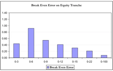
Trying to understand better these results, we display now in the following tables and Figure 5 the same results but for equity tranches. We observe on this graph that the error is maximum for the tranche 0%-6% which correspond to our empirical finding (see Figure 1) that the approximation error is maximum near the expected loss of the portfolio (equal here to 4.3%).
Attach Detach Output REC Mixte 0% 3% Default Leg 2.1744% 2.1752% Level 323.2118% 323.2634% Break Even 22.4251% 22.4295% 0% 6% Default Leg 2.7813% 2.7836% Level 383.4886% 383.5114% Break Even 12.0878% 12.0969% 0% 9% Default Leg 2.9218% 2.9240% Level 408.7648% 408.7853% Break Even 7.9422% 7.9476% 0% 12% Default Leg 2.9877% 2.9900% Level 422.1122% 422.1302% Break Even 5.8984% 5.9025% 0% 15% Default Leg 3.0282% 3.0303% Level 430.3624% 430.3788% Break Even 4.6909% 4.6940% 0% 22% Default Leg 3.0785% 3.0807% Level 441.1148% 441.1280% Break Even 3.1723% 3.1744% 0% 100% Default Leg 3.1388% 3.1410% Level 456.3206% 456.3293% Break Even 1.1464% 1.1472% Error 0-3 0.44 0-6 0.92 0-9 0.55 0-12 0.41 0-15 0.31 0-22 0.21 0-100 0.08 4.6 Sensitivity analysis
We are finally interested in calculating the sensitivity with respect topj. As for the Greek of the classical option theory, direct approximations using the finite difference method implies large errors. We hence propose the following procedure.
Letltj =ωj(1−Rj)I{τj≤t}. Then for all j= 1,· · ·, n,
(lt−k)+=I{τj≤t} X i:i6=j lit+ωj(1−Rj)−k ++I{τj>t} X i:i6=j lit−k +.
As a consequence, we may write
E[(lt−k) +|U] =F(pj, U)E h X i:i6=j lti+ωj(1−Rj)−k + Ui + 1−F(pj, U) Eh X i:i6=j lti−k + Ui.
Break Even Error on Equity Tranche 0.00 0.20 0.40 0.60 0.80 1.00 1.20 1.40 0-3 0-6 0-9 0-12 0-15 0-22 0-100
Break Even Error
Figure 5: Break even error for the equity tranches expressed in bp. Since the only term which depends onpj is the functionF(pj, U), we obtain
∂C(t, k) ∂pj = Z 1 0 du∂1F(pj, u)E h X i:i6=j lit+ωj(1−Rj)−k +− X i:i6=j lit−k + U =ui (10) where we compute the call spread using the mixed approximation for the partial total loss.
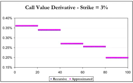
We test this approach in the case whereR= 0 on a portfolio of 100 names such that one fifth of the names have a default probability of 25 bp, 50 bp, 75 bp, 100 bp and 200 bp respectively for an average default probability of 90 bp. We compute the derivatives of call prices with respect to each individual name probability according to the formula (10) and we benchmark this result by the sensitivities given by the recursive methodology.
We find out that in all tested cases (strike ranging from 3% to 20%) the relative error on these derivatives is less than 1% except for strike higher than 15% for which the relative error is around 2%. Note however that in this case the absolute error is less than 0.1 bp for derivatives whose value is ranging from 2 bp to 20 bp. In Figure 6 we plot these derivatives for a strike value of 3% computed using the recursive and approximated methodology. We may remark that the approximated methodology always overvalue the derivatives value. However in the case of a mezzanine tranche (call spread) this effect will be offset. We consider these results as very satisfying.
Call Value Derivative - Strike = 3%
0.15% 0.20% 0.25% 0.30% 0.35% 0.40% 0 20 40 60 80 100 Recursive ApproximatedFigure 6: Derivatives with respect to individual name default probability using the recursive and approximated methodology.
5
Conclusion
We propose in this paper a combination of first order Gauss and Poisson approximations. Various numerical tests have been effectuated. Notably, we have provided an empirical threshold for choosing between the two ap-proximations. Comparisons between other numerical methods (saddle-point, Monte Carlo and recursive) show that our method provides very satisfactory results when computing prices and sensitivities for CDOs tranches . Fur-thermore, it outperforms in terms of computation time thanks to explicit formulas of correctors.
Further research work consists in some extensions where we hope to treat random recovery rates when using the Poisson approximation. In the framework of Stein’s method and zero bias transformation, this may involve certain alternative distribution other than the Poisson one.
6
Appendix
Theorem 2.1 and Theorem 2.2 are obtained through Stein’s method and zero bias transformation. We now present the theoretical framework and proofs for both theorems.
6.1 Zero bias transformation and Stein’s method
Stein’s method is an efficient tool to study the approximation problems. In his pioneer paper, Stein [20] first proposed this method to study the Gauss approximation in the central limit theorem. The method has been extended to the Poisson case by Chen [6]. In this framework, the zero bias transformation has been introduced by Goldstein and Reinert [12] for the Gaussian distribution, which provides practical and concise notation for the estimations.
Generally speaking, the zero bias transformation is characterized by some functional relationship implied by the reference distributions, Gauss or Pois-son, such that the “distance” between one distribution and the reference distribution can be measured by the “distance” between the distribution and its zero biased one.
6.1.1 The Gaussian case
In the Gaussian case, the zero bias transformation is motivated by the fol-lowing observation of Stein: a random variable (r.v.) Z has the central normal distribution N(0, σ2) if and only if E[Zf(Z)] = σ2E[f′(Z)] for all
regular enough functions f. In a more general context, for any mean zero r.v. X of variance σ2>0, a r.v. X∗ is said to have its zero biased
distribu-tion if the following reladistribu-tionship (11) holds for any funcdistribu-tionf such that the expectation terms are well-defined
E[Xf(X)] =σ2E[f′(X∗)]. (11)
The distribution of X∗ is unique with density function given by p
X∗(x) = σ−2E[XI{X>x}].
The central normal distribution is invariant by the zero bias transforma-tion. In fact, X∗ and X have the same distribution if and only if X is a
normal variable of mean zero.
For any given function h, the error of the Gaussian approximation of
E[h(X)] can be estimated by combining the Stein’s equation
xf(x)−σ2f′(x) =h(x)−Φσ(h), (12) where Φσ(h) is given by (1). By (11) and (12), we have
E[h(X)]−Φσ(h) =E[Xfh(X)−σ2fh′(X)]
=σ2E[fh′(X∗)−fh′(X)]≤σ2kfh′′kE[|X∗−X|]. (13)
where fh is the solution of (12). Here the property of the functionfh and the difference betweenX andX∗ are important for the estimations.
The Stein’s equation can be solved explicitly. If h(t) exp(− t2
2σ2) is
inte-grable on R, then one solution of (12) is given by
fh(x) = 1 σ2φ σ(x) Z ∞ x (h(t)−Φσ(h))φσ(t)dt (14)
whereφσ(x) is the density function ofN(0, σ2). The functionf
his one order more differentiable thanh. Stein has established thatkfh′′k ≤2kh′k/σ2 ifh is absolutely continuous.
For the term X −X∗, the estimations are easy when X and X∗ are
independent by using a symmetrical term Xs = X −X˜ where Xe is an independent duplicate ofX: E[|X∗−X|k] = 1 2(k+ 1)σ2E |Xs|k+2, ∀k∈N +. (15)
For the sum of independent random variables, Goldstein and Reinert [12] have introduced a construction of zero bias transformation using a random index design to choose the weight of each summand variable.
Proposition 6.1 (Goldstein and Reinert) LetXi (i= 1, . . . , n)be
indepen-dent zero-mean r.v. of finite varianceσ2
i >0andXi∗ having theXi-zero
nor-mal biased distribution. We assume that( ¯X,X¯∗) = (X1, . . . , Xn, X1∗, . . . , Xn∗)
are independent r.v. LetW =X1+· · ·+Xn and denote its variance byσW2 .
We also use the notationW(i)=W−X
i. Let us introduce a random indexI
independent of( ¯X,X¯∗)such thatP(I =i) =σi2/σ2W. ThenW∗=W(I)+XI∗
has theW-zero biased distribution.
Although W and W∗ are dependent, the above construction based on a
random index choice enables us to obtain the estimation ofW −W∗:
E|W∗−W|k= 1 2(k+ 1)σ2W n X i=1 E|Xis|k+2, ∀k∈N+. (16)
6.1.2 The Poisson case
The Poisson case is similar to the Gaussian one. Recall that Chen [6] has ob-served that a non-negative integer-valued random variable Λ of expectation λfollows the Poisson distribution if and only ifE[Λg(Λ)] =λE[g(Λ + 1)] for
any bounded function g. Similarly as in the Gaussian case, let us consider a random variableY taking non-negative integer values andE[Y] =λ <∞.
A r.v. Y∗ is said to have the Y-zero Poisson biased distribution if for any functiong such thatE[Y g(Y)] exists, we have
The Stein’s Poisson equation is also introduced by Chen [6]:
yg(y)−λg(y+ 1) =h(y)− Pλ(h) (18) where Pλ(h) = E[h(Λ)] with Λ ∼ P(λ). Hence, we obtain the error of the
Poisson approximation
E[h(V)]−Pλ(h) =EV gh(V)−λVgh(V+1)=λVEgh(V∗+1)−gh(V+1)
(19) where V is a non-negative integer-valued r.v. with expectation λV, the functiongh is the solution of (18) and is given by
gh(k) = (k−1)! λk ∞ X i=k λi i! h(i)− Pλ(h) . (20)
It is unique except at k = 0. However, the value g(0) does not enter into our calculations afterwards.
We consider now the sum of independent random variables. Let Yi(i= 1,· · · , n) be independent non-negative integer-valued r.v. with positive ex-pectationsλi andYi∗having theYi-Poisson zero biased distribution. Denote byV =Y1+· · ·+Yn andλV =E[V]. LetI be a random index independent of ( ¯Y ,Y¯∗) satisfying P(I =i) =λi/λV. Then V(I)+YI∗ has theV-Poisson zero biased distribution whereV(i) =V −Y
i.
For any integer l ≥ 1, assume that Y and Yi have to up (l+ 1)-order moments. Then E[|Y∗−Y|l] = 1 λE Y|Ys−1|l, E[|V∗−V|l] = 1 λV n X i=1 EYi|Yis−1|l.
Finally, recall that Chen has established k∆ghk ≤ 6khkmin λ−
1
2,1 with
which we obtain the following zero order estimation
|E[h(V)]− Pλ V(h)| ≤6khkmin 1 √ λV ,1 n X i=1 EYi|Yis−1|. (21)
There also exist other estimations of error bound (e.g. Barbour and Eagleson [3]). However we are more interested in the order than the constant of the error.
6.2 Proof of Theorem 2.1 and 2.2
We shall use in the sequel without comment the notation introduced in Section 6.1.
6.2.1 The normal case: Theorem 2.1
We now give the explicit form of the corrected approximation error and the proof to establish it. With the notation of Theorem 2.1, the corrected error boundα(h, X1,· · ·, Xn) is given by E[h(W)]−Φσ W(h)−Ch ≤fh(3) 1 12 n X i=1 E|Xis|4+ 1 4σ2 W n X i=1 E[Xi3] n X i=1 E|Xis|3+ 1 σW v u u t n X i=1 σi6 . (22) Note that the existence offh(3) requires thath is second order derivable.
Proof. By taking first order Taylor expansion, we obtain
E[h(W)]−Φσ W(h) =σ 2 WE[fh′(W∗)−fh′(W)] =σ2WE[fh′′(W)(W∗−W)] +σ2WE h fh(3) ξW + (1−ξ)W∗ξ(W∗−W)2i (23) whereξ is a random variable on [0,1] independent of allXiandXi∗. Firstly, we notice that the remaining term is bounded by
Ehf(3) h ξW+(1−ξ)W∗ ξ(W∗−W)2i≤ fh(3) 2 E[(W ∗−W)2]≤ fh(3) 12σW2 n X i=1 E|Xis|4. (24) Secondly, we consider the first term of equation (23). Since XI∗ is inde-pendent ofW, we have
E[fh′′(W)(W∗−W)] =E[fh′′(W)(XI∗−XI)] =E[XI∗]E[fh′′(W)]−E[fh′′(W)XI].
(25) For the first term E[X∗
I]E[fh′′(W)] of (25), we write it as the sum of two parts E[XI∗]E[fh′′(W)] =E[XI∗]Φσ W(f ′′ h) +E[XI∗]E[fh′′(W)−ΦσW(f ′′ h)]. The first term E[X∗
I]ΦσW(f
′′
h) of the right-hand side is the candidate of the corrector. For the second term, we apply the zero order estimation and get
E[XI∗]E[fh′′(W)]−Φσ W(f ′′ h)≤ fh(3) 4σ4 W n X i=1 E[Xi3] n X i=1 E|Xis|3. (26)
For the second term E[f′′
h(W)XI] of (25), we use a technique of condi-tional expectation by observing thatE[f′′
h(W)XI] =E f′′ h(W)E[XI|X,¯ X¯∗] .
Then by the Cauchy-Schwartz inequality, E[fh′′(W)XI] =covfh′′(W),E[XI|X,¯ X¯∗]≤ 1 σW2 q Var[f′′ h(W)] v u u t n X i=1 σ6 i.
Notice that Var[fh′′(W)] = Var[fh′′(W)−fh′′(0)] ≤ E[(fh′′(W)−fh′′(0))2] ≤
kfh(3)k2σW2 . So E[fh′′(W)XI] ≤ kf (3) h k σW v u u t n X i=1 σ6 i . (27)
Finally, it suffices to write
E[h(w)]−Φσ W(h) =σ 2 W E[XI∗]Φσ W(f ′′ h) +E[XI∗] E[fh′′(W)]−Φσ W(f ′′ h) −E[fh′′(W)XI] +σ2WE h fh(3) ξW + (1−ξ)W∗ξ(W∗−W)2i. (28) Combining (24), (26) and (27), we let the corrector to beCh =σ2WE[XI∗]ΦσW(f
′′
h) and we deduce the error boundα(h, X1,· · · , Xn) as in (22).
The last step is to use the invariant property of the normal distribution under zero bias transformation and the Stein’s equation to obtain
σ2WΦσW(f ′′ h) = ΦσW(xf ′ h) = 1 σ2 W ΦσW ( x 2 3σ2 W −1)xh(x).
6.2.2 The Poisson case: Theorem 2.2
Proof. Let us first recall the discrete Taylor formula. For any integersxand any positive integerk≥1,
g(x+k) =g(x) +k∆g(x) + k−1
X
j=0
(k−1−j)∆2g(x+j).
Similar as in the Gaussian case, we apply the above formula to right-hand side ofE[h(V)]− Pλ
V(h) =λVE[gh(V
∗+ 1)−gh(V + 1)] and we shall make
aroundV(i) for the following three terms respectively and obtain Egh(V∗+ 1)−gh(V + 1)−∆gh(V + 1)(V∗−V) = n X i=1 λi λV Egh(V(i)+ 1) +Yi∗∆gh(V(i)+ 1) + Y∗ i−1 X j=0 (Yi∗−1−j)∆2gh(V(i)+ 1 +j) −Egh(V(i)+ 1) +Yi∆gh(V(i)+ 1) + YXi−1 j=0 (Yi−1−j)∆2gh(V(i)+ 1 +j) −E∆gh(V(i)+ 1)(Yi∗−Yi) + YXi−1 j=0 (Yi∗−Yi)∆2gh(V(i)+ 1 +j)
which implies that the remaining term is bounded by
Egh(V∗+ 1)−gh(V + 1)−∆gh(V + 1)(V∗−V) ≤ k∆2ghk n X i=1 λi λV E hY∗ i 2 ] + Yi 2 i +E|Yi(Yi∗−Yi)| ! . We then make decomposition
E∆gh(V + 1)(V∗−V)=Pλ V(∆gh(x+ 1))E[Y ∗ I −YI] + cov YI∗−YI,∆gh(V + 1) + E[∆gh(V + 1)]− Pλ V(∆gh(x+ 1)) E[YI∗−YI]. (29) Similar as in the Gaussian case, the first term of (29) is the candidate of the corrector. For the second term, we use again the technique of conditional expectation and obtain
cov∆gh(V + 1), YI∗−YI ≤ λ1 V Var∆gh(V + 1) 1 2 Xn i=1 λ2iVar[Yi∗−Yi] 1 2 . For the last term of (29), we have by the zero order estimation
E[∆gh(V+1)]−Pλ V(∆gh(x+1)) E[YI∗−YI]≤ 6k∆ghk λV Xn i=1 E[Yi|Yis−1|] 2 .
It remains to observe that PλV(∆gh(x+ 1)) =
1
2PλV(∆
2h) and let the
cor-rector to be
ChP = λV
2 PλV(∆
2h)E[Y∗
I −YI].
below E[h(V)]− Pλ V(h)−C P h ≤ k∆2ghk n X i=1 λiE h |Yi∗−Yi| |Yi∗−Yi| −1 i + Var∆gh(V + 1) 1 2 Xn i=1 λ2iVar[Yi∗−Yi] 1 2 + 6k∆ghk Xn i=1 E[Yi|Yis−1|] 2 (30) wherek∆ghk ≤6khkand k∆2ghk ≤2k∆ghk.
References
[1] Andersen, L., J.Sidenius and S.Basu (2003), All your hedges in one basket. Risk, Nov, 2003, 67-72.
[2] Antonov, A., S. Mechkov and T. Misirpashaev (2005), Analytical tech-niques for synthetic CDOs and credit default risk measures, Working paper, NumeriX.
[3] Barbour, A. D. and Eagleson, G. K. (1983), Poisson approximation for some statistics based on exchangeable trials, Advances in applied probability, 15 (3), 585-600.
[4] Burtschell, X., J. Gregory and J.-P. Laurent (2007), Beyond the Gaus-sian copula: stochastic and local correlation, Journal of Credit Risk, 3(1), 31-62.
[5] Brasch, H.-J. (2004), A note on efficient pricing and risk calculation of credit basket products. Working paper, TD Securities.
http://www.defaultrisk.com/pp$_$crdrv$_$54.htm
[6] Chen, L.H.Y (1975), Poisson approximation for dependent trials. An-nals of probability, 3, 534-545.
[7] Chen, L.H.Y and Q.-M. Shao (2001), A non-uniform Berry-Esseen bound via Stein’s method. Probability theory and related fields, 120, 236-254.
[8] Chen, L.H.Y. and Q.-M. Shao (2005), Stein’s method for normal ap-proximation, An introduction to Stein’s method, Lecture notes series Vol.4, University Singapore, 1-59.
[9] Diener, F. and M. Diener (2004), Asymptotics of price oscillations of a European call option in a tree model. Mathematical finance, 14(2) 271-293.
[10] El Karoui, N. and Y. Jiao (2008), Stein’s method and zero bias transfor-mation for CDOs tranche pricing, to appear inFinance and Stochastics. [11] Finger, C.C. (1999), Conditional approches for CreditMetrics portfolio
distributions. CreditMetrics Monitor April 1999, 14-33.
[12] Goldstein, L. and G. Reinert (1997), Stein’s method and the zero bias transformation with application to simple random sampling.Annals of applied probability, 7, 935-952.
[13] Gordy, M. B. (2003), A risk-factor model foundation for ratings-based bank capital rules.Journal of Financial Intermediation, 12(3):199-232. [14] Gregory, J. and J.-P. Laurent (2003), I will survive.Risk, 16(6). [15] Hull, J. and A. White (2004), Valuation of a CDO and annth-to-default
CDS without Monte Carlo simulation, Working paper, University of Toronto,
[16] Martin, R., K. Thompson and C. Browne (2001), Taking to the saddle.
Risk, June.
[17] Martin, R., K. Thompson and C. Browne (2001), VaR: who contributes and how much? Risk, June.
[18] Merino, S and M. Nyfeler (2002), Calculating portfolio loss. Risk, Au-gust.
[19] Petrov, V. V. (1975), Sums of independent random variables. Springer-Verlag, New York.
[20] Stein, C. (1972), A bound for the error in the normal approxima-tion to the distribuapproxima-tion of a sum of dependent random variables,Proc. sixty Berkely symp. math. statis. probab., University of California Press, Berkeley pp. 583-602.
[21] Stein, C. (1986), Approximate computation of expectations. IMS, Hay-ward, CA.
[22] Tanaka, K., T. Yamada and T. Watanabe (2005), Approximation of interest rate derivatives’ prices by Gram-Charlier expansion and bond moments. Working paper, Bank of Japan.
[23] Turc, J. (2005), Valoriser les CDO avec un smile. Working paper, Recherche Cr´edit, Soci´et´e G´en´erale.
[24] Vasicek, O. (1991), Limiting loan loss probability distribution. Working paper, Moody’s KMV.
[25] Wood, A., J. G. Booth and R.W. Butler (1993), Saddlepoint approxi-mations to the CDF of some statistics with nonnormal limit distribu-tions. Journal of the American Statisical Association, 88(422):680-686. Moody’s KMV.