Learning Model-Ensemble Policies with Genetic Programming

Herausgeber: T. Bartz-Beielstein, W. Konen, H. Stenzel, B. Naujoks

Learning Model-Ensemble

Policies with Genetic

Programming

Oliver Flasch, Martina Friese, Martin Zaefferer,

Thomas Bartz-Beielstein, J¨

urgen Branke

Programming

Oliver Flasch1_{, Martina Friese}1_{, Martin Zaefferer}1_, Thomas Bartz-Beielstein1_{, and J¨urgen Branke}2

1 _{Faculty for Computer and Engineering Sciences}

Cologne University of Applied Sciences, 51643 Gummersbach, Germany

[email protected]

2

Warwick Business School, University of Warwick Coventry, CV4 7AL, UK

[email protected]

Abstract. We propose to apply typed Genetic Programming (GP) to the problem of finding surrogate-model ensembles for global optimization on compute-intensive target functions. In a model ensemble, base-models such as linear models, random forest models, or Kriging models, as well as pre- and post-processing methods, are combined. In theory, an opti-mal ensemble will join the strengths of its comprising base-models while avoiding their weaknesses, offering higher prediction accuracy and ro-bustness. This study defines a grammar of model ensemble expressions and searches the set for optimal ensembles via GP. We performed an extensive experimental study based on 10 different objective functions and 2 sets of base-models. We arrive at promising results, as on unseen test data, our ensembles perform not significantly worse than the best base-model.

Keywords: Ensemble Methods, Genetic Programming, Surrogate-Model-Based Optimization

1

Introduction

The application of surrogate-model based methods for the purpose of solving cost extensive and time consuming optimization problems is an established tech-nique. Surrogate models, as employed in methods like Efficient Global Optimiza-tion (EGO) [19] or Sequential Parameter OptimizaOptimiza-tion (SPO) [1] offer several advantages. While their main goal is often to reduce the number of costly tar-get function evaluations, one can also benefit from the information surrogate models provide on the problem. This can include information on the shape of the optimized landscape, interactions between parameters or their individual importance.

A question that often arises with such approaches is the choice of the model-ing technique (e.g., tree-based, Support Vector Machines or Krigmodel-ing). This paper

will use ”base-models” to refer to such different model types. Depending on the task at hand, a certain individual base-model might be most promising. In many cases however it may be unclear which of several candidates is best suited. For instance, one base-model might provide better global approximation than an-other, while another base-model can handle discontinuous regions of the design space with more ease. Thus it is of interest to develop methods with which to choose from or combine substantially different base-models.

Relevant cross references to similar problems as well as previous studies on this issue are reviewed in Sec. 2.

In this very first step towards learning a meaningful ensemble policy, a Ge-netic Programming (GP) system is used to combine the different models with very simple operators. The methods to this end are introduced in Sec. 3. We limit ourselves to the modeling stage, due to the complexity of the problem. Employ-ing generated ensemble policies in an actual optimization framework will remain for a detailed investigation in following publications.

Thus, our approach is tested for its success in modeling simple numerical test functions. The problem setup, including test functions and employed modeling techniques, are described in Sec. 4. Experiment results are given in Sec. 5 and analyzed in Sec. 6. This text closes with a summary and outlook in Sec. 7.

2

Previous Research

Ensembles are not a new topic, neither in modeling nor in surrogate model supported optimization.

As the costly optimization problems at hand warrant only very sparse sam-pling of data, some classical ensemble approaches like bootstrap aggregating (bagging) [2] or boosting [20, 28] are not well applicable. Also, bagging is often, although not always [22, 6], employed to build ensembles of homogeneous base-models, i.e. models of the same type (e.g., only tree or only linear). In a similar way boosting has been used to combine homogeneous base-models to a stronger set of models, for instance as applied in evolutionary optimization by Holeˇna et al. [17].

With a different concept, Ong et al. [27] combined homogeneous base-models by building them locally around individuals of an evolutionary algorithm’s pop-ulation, thus building different models in different regions of the design space. Another approach to splitting the design space is that of Gramacy et al. [15]. There, trees that split the design space are learned, applying Gaussian process or linear models in the various divisions.

Two different ensemble policies have been tested by Lim et al. [26] for the purpose of enhancing a Surrogate Assisted Memetic Algorithm. They combined base-models either by aggregation or by selecting the best solution from each model for evaluation on the real target function.

Focusing on a heterogeneous set of base-models, Gorissen et al. [14] combine models using a genetic algorithm. In their implementation, ensembles occur when

two model types are selected for recombination. The ensembles created are sim-ply an averaged combination of the models.

Several alternative approaches were recently investigated by Friese et al. [12]. They grouped approaches into two categories, single-evaluation and multiple-evaluation. Single-evaluation approaches view the problem of choosing a model from the ensemble as a multi armed bandit problem [13]. That means, only infor-mation from one model is chosen in each sequential optimization step. Multiple-evaluation approaches train every model in each step, thus using information from all of them.

The single-evaluation approach is also taken by Hess et al. [16], who introduce their algorithm termed PROGRESS. PROGRESS is an enhanced algorithm for solving multi armed bandit problems, specifically adapted to the problem of selecting a surrogate model for optimization.

There are further approaches, including some not solely intended for being employed in surrogate model optimization.

One example is the approach of Frayman et al. [10]. Frayman [10] et. al use a neural network (Multi Layer Perceptron MLP) to train an ensemble combining linear, MLP, logistic regression and k-nearest neighbor models. This approach can be classified as a variation of stacked generalization, or model stacking [29, 3].

3

Methods

This section describes the various methods used in this work, including model ensembles and model combination policies. It is shown how model combination policies are evaluated and how they are evolved by GP.

3.1 Model Ensembles

It still remains unclear how an ideal policy would combine information from fundamentally different base-models in a meaningful way. While theoretical con-siderations or ideas from other fields (i.e. multi armed bandit problems) do yield Ensemble-Policies that work to some extend, we would like to suggest a way to learn such policies in a less constricted environment.

The idea presented here attempts to do so with a GP approach. That is, the different models are viewed as parameters in a symbolic regression problem.

With the terms of Friese et al. we will herein attempt to learn a policy for a multiple-evaluation approach [12] Multiple-evaluation approaches train every model in each step, combining or selecting from the information yielded. As single evaluation approaches need several optimization steps to learn the right behavior, they may often be infeasible for the costly problems of concern in surrogate model based optimization.

In this paper we call the set of available base-models M. A specific base-model will be referred to asmi, where i represents the index of the model type (e.g., 1 is a linear model, 2 is a Kriging model, etc.). During experiments, each

mi will be trained on a fixed training data set and yield a vector of responsesyi for a second, independent validation data set.

A policy combining severalmiwill be referred to asπk. Here,krepresents a counter, as several policies can be learned, for instance by restarting a GP run with a different seed.

In the following, the modelsmi, as well as policiesπk are described as real-valued functions defined in d-dimensional bounded parameter space D ⊂ Rd. The dimensionality d, as well as the bounds, or region of interest, of D are dependent on the objective function.

x d t xd<t xd≥t

mean

LM

x

mean

*

RF

x

1.88

decision

x

2

−0.59 −1.75

0.03

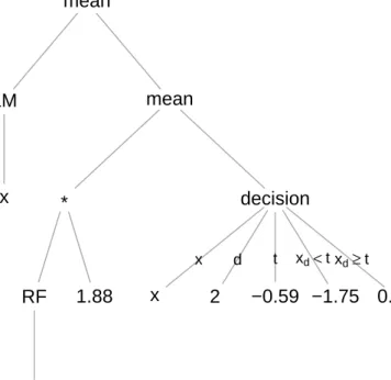
Fig. 1.Example of a GP-generated policy shown as an expression tree.

Fig. 1 shows the expression tree of the following GP-evolved example policy: mean[LM(x),mean[RF(x)×1.88,decision(x,2,−0.59,−1.75,0.03)]]

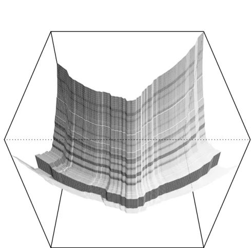
This policy combines a linear model (LM) with a random forest model (RF) by calculating the arithmetic mean of the model outputs. The RF output is further post-processed by scaling and mixing (also via arithmetic mean) with the output of a simple GP-evolved decision tree. As we are only using 2D test functions in this study, base-models and model ensembles can be visualized as surface plots.

In these plots, the first dimension of the bounded parameter spaceDis assigned to the X (width) axis, the second dimension ofD to the Y (depth) axis and the model output to the Z (height) axis.

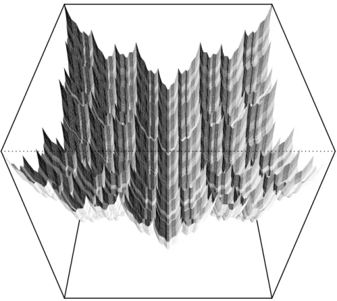
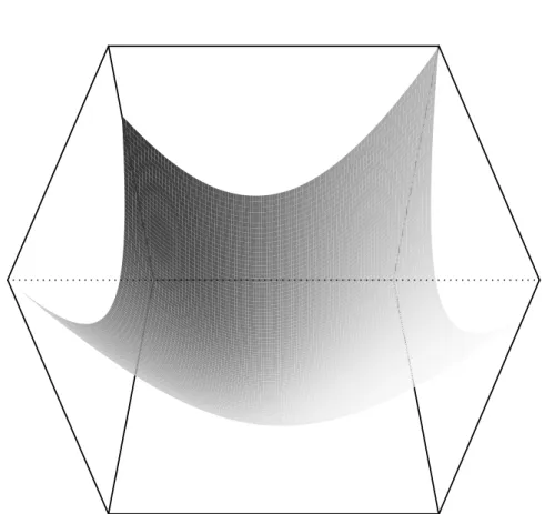
As an example, we applied the ensemble policy of Fig. 1 to the 2D Weierstrass function with the bounds (domain) shown in Tab. 1. Fig. 2 provides a surface plot of this test function. As our example policy refers to the LM and RF base-models, both models have to be fitted to training data. Surface plots of these base-model fits are shown in Fig. 3 and Fig. 4, respectively. Based on these fits, the output of our example policy is shown as a surface plot in Fig. 5.

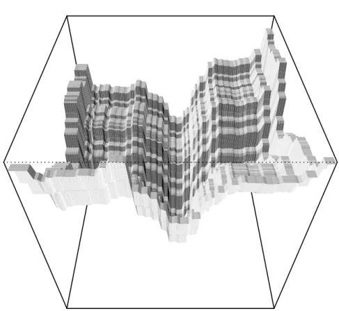
Fig. 4. Surface plot of a random forest (RF) model fit of the 2D Weierstrass test function.

Fig. 5.Surface plot of an ensemble fit of the 2D Weierstrass test function based on the policy shown in Fig. 1. The base-model fits used in the ensemble are shown in Fig. 3 and Fig. 4.

3.2 Typed Genetic Programming

To apply GP to the problem of finding model combination policiesπk given as symbolic expressions for combining base modelsmi, we have to define

i) a quality measure for policy expressions (fitness function), ii) the set of valid policy expressions,

iii) the set of GP variation operators (mutation and recombination), iv) the GP search heuristic and its parameters.

As a quality measure, we use the Scaled Root Mean Squared Error (SRMSE) on an independent validation data set, as introduced in Sec. 4.3. For GP, SRMSE is a particularly well-suited, as the GP system does not have to fit constants exactly.

We represent combination policies as symbolic expressions (i.e. formulas). The set of valid policy expressions is defined by the grammar given in Extended Backus-Naur Form (EBNF) shown in Fig. 6 [18]. Here, terminal symbols are shown in a regular typeface, non-terminal symbols are shown in italics. The start symbol of the grammar is marked by enclosing it in a box.

According to this grammar, a policy expression is either a base policy expres-sion, the sum, product, difference, arithmetic mean or minimum of two policy expressions, or a branching ”decision” expression. Decision expressions split the input space into two subspaces that can then be handled by sub-policies. The in-put space is split axis-parallel. The split dimension is given by a constant indexi, the split threshold is given by a constant scalar between -1 and 1, which is scaled to the lower and upper bounds of the region of interest of the selected dimension. If the ith component of the input vector is strictly less than the threshold, the first policy is applied, otherwise, the second policy is applied. Note that deci-sion expresdeci-sions can be nested. Decideci-sion expresdeci-sions enable policies that apply different combinations of base-models to different areas of the parameter space D.

The set of valid combination policies as defined in Fig. 6 was chosen some-what arbitrary as a compromise of GP search space size and policy expression expressiveness. Possibly interesting additions left for further work are non-linear transformations of the parameter spaceDas well as of the objective (i.e. model output) spaceR.

In our GP system, policy expressions are represented as trees annotated with type information. Therefore, standard tree-based GP algorithms can be applied with minimal modifications to respect type constraints.

We used the open source R-based GP system RGP [8] in release version 0.3-1 for all our experiments. Source code and documentation can be downloaded at

http://rsymbolic.org/projects/show/rgpandhttp://cran.r-project.org/. Standard Koza-style [23,?] typed GP operators are used used for GP individual (i.e. policy expression) initialization, mutation and recombination. We used the default GP operator set for typed GP as implemented in RGP version 0.3-1. See the RGP documentation for details. As GP search heuristic, or concrete GP algorithm, we used the default of RGP 0.3-1, that is a modern Pareto GP search

policy =base policy |policy+policy |policy×policy |policy−policy |mean(policy,policy) |min(policy,policy)

|decision(point,index,threshold,policy,policy) base policy=base model(point)

base model=fast base model|KF|MLP|SVM fast base model=LM|MARS|RF

point=x|constant vector index=1|2| · · · |d

threshold=constant scalar∈[−1,1]

Fig. 6.EBNF-Grammar Defining the Set of Valid Policy Expressions. Terminal sym-bols are shown in a regular typeface, non-terminal symsym-bols are shown initalics. The start symbol of the grammar is marked by a box .

heuristic with age layering for population diversity preservation. See the RGP documentation for details.

We disabled the complexity criterion of the search heuristic as in this stage of experimentation, we are interested in identifying the best possible policy expres-sions, regardless of complexity. Policy expressions larger than a given threshold are suppressed by the fitness function simply by assigning a very large (i.e. bad) fitness value. The concrete parameters of the GP system are described in the following Section on experiment setup.

4

Experiment Setup

All experiments are performed using the free software environment for statistical computation, R3_.

4.1 Objective Functions

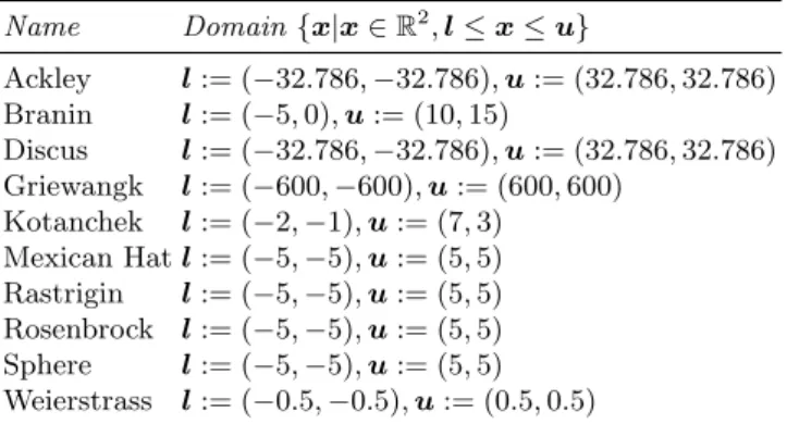
All of the employed test functions are taken from thesoobench_Rpackage. These functions and their respective domains are shown in Tab. 1.

All scalable functions are used in their two-dimensional form. This was chosen for simplicity of this very first step, as well as for the possibility to visually inspect

3

Ras well as all employed packages, includingrgpandSPOT, are available at http: //cran.r-project.org/

Table 1.Test Functions Used in this Study Name Domain{x|x∈R2,l≤x≤u} Ackley l:= (−32.786,−32.786),u:= (32.786,32.786) Branin l:= (−5,0),u:= (10,15) Discus l:= (−32.786,−32.786),u:= (32.786,32.786) Griewangk l:= (−600,−600),u:= (600,600) Kotanchek l:= (−2,−1),u:= (7,3) Mexican Hatl:= (−5,−5),u:= (5,5) Rastrigin l:= (−5,−5),u:= (5,5) Rosenbrock l:= (−5,−5),u:= (5,5) Sphere l:= (−5,−5),u:= (5,5) Weierstrass l:= (−0.5,−0.5),u:= (0.5,0.5)

the quality of the created model ensembles. Visual inspection is of interest due to the fact that an ideal measure of model quality for this purpose does not exist. The function’s lower and upper boundaries as given by the soobench package are used in the following experiments.

4.2 Surrogate Models for Ensemble

The choice of surrogate models will have a great influence on the experimental outcome. Using strong base-models like Kriging might lead to ensembles that can at best perform as good as those strong base-models. This however has to be accepted as part of the problem.

More importantly, using too many base-models might blow up the problem complexity quite significantly. At the same time one is interested in having as many model types as possible, to identify the usefulness of their different features in an ensemble environment.

We therefore selected six surrogate modeling techniques which should cover a wide variety of features and limitations:

LM Linear models (LM) with up to second order terms, build with thersmR package by Lenth [25]. This model’s simple structure does not only warrant a fast training, but also easy interpretability for the user. It is however unable to approximate multi-modal landscapes very well.

RF Random Forest implementation from the_R packagerandomForest which is based on Breiman and Cutler’s original Fortran code for classification and regression [4]. RF is usually a good global approximator, avoids over-fitting and can handle categorical variables very well. However, the landscape as approximated by RF will be divided into several partitions with constant function values. This and the discontinuity of the RF model can make it problematic for use in an optimization environment.

MARS Multivariate Adaptive Regression Splines (MARS) [11] provided by the

earth R package. MARS allow for better approximations LM while still being relatively well interpretable.

MLP Multi Layer Perceptron (MLP) [24] is a type of neural network, imple-mented in the_Rpackagemonmlp. MLP models can be very flexible universal approximators, but may require a lot of time for training.

SVM A Support Vector Machine implementation in the package e1071 using LIBSVM [5]. SVM models are versatile and can still work even on high dimensional problems. They are however sensitive to several parameters that require tuning, which leads to a larger computational burden.

KF Kriging implementation shipped withSPOT_Rpackage, based on the original Matlab code by Forrester et al. [9]. Kriging is a very flexible approximator for continuous functions. In addition to the estimation of the function value, it also provides an estimation of the error. This feature however is not employed in this study.

Some of those models can themselves be considered ensembles. For instance, RF is a homogeneous ensemble of trees.

The base-models listed above were combined in two different sets for the experiment, M1 and M2. The small set M1 consists only of the more simple and faster to train models (LM, RF, MARS). The full setM2 consists of all six models. Therefore, every GP run on a test function was done twice, i.e. once for each of the two sets.

4.3 Data-Usage

To receive unbiased results, the usage of data during the experiment has to be planned carefully. We do 48 repeats of each GP run, each with different random number generator seeds. This is performed on each of the ten test functions. As specified in the previous section, each experiment is also performed once with the small, and once with the full set of base-models. This results in 48∗10∗2 = 960 GP runs.

For each of these runs we employ the following concept of data-usage 1. TrainingEach base-model is trained on a Latin Hypercube Design (LHD)

consisting of 20 points in the design space, which was evaluated on the corresponding test function. This data set will be referred to as LHDi1, whereiis the index for each of the 48 repeats.

2. ValidationEach policy created during the GP run receives a fitness value. This is evaluated based on an error measure, as described in Sec. 4.4. The error measure is evaluated on a second LHD consisting of 40 points, referred to asLHDi2

3. TestFinally, each final best policyπhas to be tested on data not seen during training or during the validation (or policy selection) phase. Therefore, each final best policy is tested on the data sets provided by the other 47 repeats of the same experiments. That is, the fitness function is invoked for each

policy, using base-models trained onLHDj₁, evaluating them on LHDj₂. Here,j is any number from one to 48, excludingi.

For each test function and model set 48 times 47 test values are received for the result analysis. As the base-models are used for a comparison in the result analysis, their fitness is evaluated in the same way.

4.4 GP Fitness Function

The fitness associated with each policyπis here based on the scaled root mean square error (SRMSE) as proposed by Keijzer [21],

SRM SE(t, y) =q_n1Pn

i=1(ti−(a+byi))2.

Here, t are the values sampled on the test function andy are the values as predicted by a base-model or an ensemble of base-models. The intercept aand the slope b are calculated by finding the zeros of the partial derivative of the error.

The SRMSE is a promising choice for automatically created policies, as it is more robust to the choice of constants than the RMSE. For instance, a simple policy consisting of the sum of two base-models mi would yield bad RMSE values, while the scaled SRMSE would correct this error by scaling the response of the policy to the range of the target function. A second advantage of SRMSE is that it will prefer policies which capture the structure of the target function. As our initial motivation is to employ such policies for optimization, capturing the structure of a target function is an important feature. Of course, this ”repair” feature of the SRMSE has to be remembered when later applying the found policies, as they will have to be scaled to provide the measured performance.

To limit the maximum size of GP-evolved policy expressions, our fitness functions associates a fitness of positive infinity to all policy expressions above a certain tree depth limit. This tree depth limit is defined as a GP parameter and given in the next subsection.

4.5 GP Parameter Settings

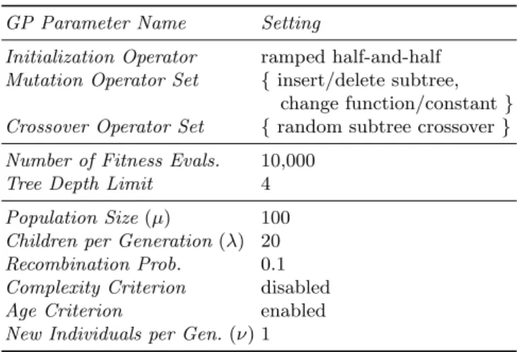
The parameter settings of all our GP experiments are summarized in Tab. 2. As already mentioned in Sec. 3.2, standard Koza-style typed GP initialization and variation operators are used. Details on these operators can be found in the RGP documentation. The maximum tree depth limit was set to 4 to suppress excessively complex policy expressions. Each GP run had a budget of 10,000 fitness function evaluations. We used a modern elitist multi-criteria evolution-ary algorithm based on the well-known NSGA-II algorithm as our GP search heuristic [7]. In addition to fitness, we added individual age as a second mini-mization criterion. Our algorithm introduces a newly initialized policy expression of age 0 into the GP population in each generation. In combination with the age minimization criterion, this strategy provides an efficient means of population

diversity preservation. Details on this algorithm can be also found in the RGP documentation.

We refrained from using a complexity criterion in this work, mainly to sim-plify result analysis and lower algorithm complexity, although we plan to add policy expression complexity as a minimization criterion in a later study.

Table 2.Parameters Settings of the GP System.

GP Parameter Name Setting

Initialization Operator ramped half-and-half Mutation Operator Set {insert/delete subtree,

change function/constant} Crossover Operator Set {random subtree crossover} Number of Fitness Evals. 10,000

Tree Depth Limit 4 Population Size(µ) 100 Children per Generation(λ) 20 Recombination Prob. 0.1 Complexity Criterion disabled Age Criterion enabled New Individuals per Gen.(ν) 1

5

Results

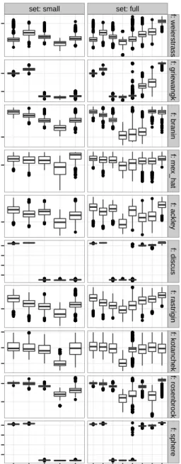
The results of the experiments are depicted in Fig. 7. It shows that the perfor-mance of the ensemble policies based on the validation data is better than any of the base-models. The performance decreases significantly when evaluated on test data. That decrease is not only significant but results into the ensemble policies being equal to or worse than the best base-model for each test function. The only exception where the policies are significantly better than the base-models on test data is the Rosenbrock function, although only on the small experimental set.

The base-models rank differently, depending on concerned test function. It was noted that Kriging showed unexpected high SRMSE values on several func-tions, that are usually very well suited for Kriging (e.g, Branin function). In fact, this could be traced back to a bug in the used implementation. The imple-mentation bug is fixed and results will be updated for a revised version of this paper.

6

Discussion

The results described in Sec. 5 reveal one problem, which is over-fitting. In its current form the ensemble policies look promising on validation data, but (with

set: small set: full ● ● ● ● ● ● ● ● ● ● ● ● ● ● ● ● ● ● ● ● ● ● ● ● ● ● ● ● ● ● ● ● ● ● ● ● ● ● ● ● ● ● ● ● ● ● ● ● ● ● ● ● ● ● ● ● ● ● ● ● ● ● ● ● ● ● ● ● ● ● ● ● ● ● ● ● ● ● ● ● ● ● ● ●●● ● ● ● ● ● ● ● ● ● ● ● ● ● ● ● ● ● ● ● ● ● ● ● ● ● ● ● ● ● ● ● ● ● ● ● ● ● ● ● ● ● ● ● ● ● ● ● ● ● ● ● ● ● ● ● ● ● ● ● ● ● ● ● ● ● ● ● ● ● ● ● ● ● ● ● ● ● ● ● ● ● ● ● ● ● ● ● ● ● ● ● ● ● ● ● ● ● ● ● ● ● ● ● ● ● ● ● ● ● ● ● ● ● ● ● ● ● ● ● ● ● ● ● ● ● ● ● ● ● ● ● ● ● ● ● ● ● ● ● ● ● ● ● ● ● ● ● ● ● ● ● ● ● ● ● ● ● ● ● ● ● ● ● ● ● ● ● ● ● ● ● ● ● ● ● ● ● ● ● ● ● ● ● ● ● ● ● ● ● ● ● ● ● ● ● ● ● ● ● ● ● ● ● ● ● ● ● ● ● ● ● ● ● ● ● ● ● ● ● ● ● ● ● ● ● ● ● ● ● ● ● ● ● ● ● ● ● ● ● ● ● ● ● ● ● ● ● ● ● ● ● ● ● ● ● ● ● ● ● ● ● ● ● ● ● ● ● ● ● ● ● ● ● ● ● ● ● ● ● ● ● ● ● ● ● ● ● ● ● ● ● ● ● ● ● ● ● ● ● ● ● ● ● ● ● ● ● ● ● ● ● ● ● ● ● ● ● ● ● ● ● ● ● ● ● ● ● ● ● ● ● ● ● ● ● ● ● ● ● ● ● ● ● ● ● ● ● ● ● ● ● ● ● ● ● ● ● ● ● ● ● ● ● ● ● ● ● ● ● ● ● ● ● ● ● ● ● ● ● ● ● ● ● ● ● ● ● ● ● ● ● ● ● ● ● ● ● ● ● ● ● ● ● ● ● ● ● ● ● ● ● ● ● ● ● ● ● ● ● ● ● ● ● ● ● ● ● ● ● ● ● ● ● ● ● ● ● ● ● ● ● ● ● ● ● ● ● ● ● ● ● ● ● ● ● ● ● ● ● ● ● ● ● ● ● ● ● ● ● ● ● ● ● ● ● ● ● ● ● ● ● ● ● ● ● ● ● ● ● ● ● ● ● ● ● ● ● ● ● ● ● ● ● ● ● ● ● ● ● ● ● ● ● ● ● ● ● ● ● ● ● ● ● ● ● ● ● ● ● ● ● ● ● ● ● ● ● ● ● ● ● ● ● ● ● ● ● ● ● ● ● ● ● ● ● ● ● ● ● ● ● ● ● ● ● ● ● ● ● ● ● ● ● ● ● ● ● ● ● ● ● ● ● ● ● ● ● ● ● ● ● ● ● ● ● ● ● ● ● ● ● ● ● ● ● ● ● ● ● ● ● ● ● ● ● ● ● ● ● ● ● ● ● ● ● ● ● ● ● ● ● ● ● ● ● ●●●● ● ● ● ● ● ● ● ● ● ● ● ● ● ● ● ● ● ● ● ● ● ● ● ● ● ● ● ● ● ● ● ● ● ● ● ● ● ● ● ● ● ● ● ● ● ● ● ● ● ● ● ● ● ● ● ● ● ● ● ● ● ● ● ● ● ● ● ● ● ● ● ● ● ● ● ● ● ● ● ● ● ● ● ● ● ● ● ● ● ● ● ● ● ● ● ● ● ● ● ● ● ● ● ● ● ● ● ● ● ● ● ● ● ● ● ● ● ● ● ● ● ● ● ● ● ● ● ● ● ● ● ● ● ● ● ● ● ● ● ● ● ● ● ● ● ● ● ● ● ● ●●●●●●●●●●●●●●●●●●●●●●●●●●●●●●●●●●●●●●●●●●●●●●● ●●●●●●●●●●●●●●●●●●●●●●●●●●●●●●●●●●●●●●●●●●●●●●●●●●●●●●●●●●●●●●●●●●●●●●●●●●●●●●●●●●●●●●●●●●●●●●●●●●●●●●●●●●●●●●●●●●●●●●●●●●●●●●●●●●●●●●●●●●●●●●●●●●●●●●●●●●●●●●●●●●●●●●●●●●●●●●●●●●●●●●●●●●●●●●●●●●●●●●●●●●●●●●●●●●●●●●●●●●●●●●●●●●●●●●●●● ● ● ● ● ● ● ● ● ● ● ● ● ● ● ● ● ● ● ● ● ● ● ● ● ● ● ● ● ● ● ● ● ● ● ● ● ● ● ● ● ● ● ● ● ● ● ● ● ● ● ● ● ● ● ● ● ● ● ● ● ● ● ● ● ● ● ● ● ● ● ●●●●_●●_●●●_●● ● ● ● ● ● ● ● ● ● ● ● ● ● ● ● ● ● ● ● ● ● ● ● ● ● ● ● ● ● ● ● ● ● ● ● ● ● ● ● ● ● ● ● ● ● ● ● ● ● ● ● ● ● ● ● ● ● ● ● ● ● ● ● ● ● ● ● ● ● ● ● ● ● ● ● ● ● ● ● ● ● ● ● ● ● ● ● ● ● ● ● ● ● ● ● ● ● ● ● ● ● ● ● ● ● ● ● ● ● ● ● ● ● ● ● ● ● ● ● ● ● ● ● ● ● ● ● ● ● ● ● ● ● ● ● ● ● ● ● ● ● ● ● ● ● ● ● ● ● ● ● ● ● ● ● ● ● ● ● ● ● ● ● ● ● ● ● ● ● ● ● ● ● ● ● ● ● ● ● ● ● ● ● ● ● ● ● ● ● ● ● ● ● ● ● ● ● ● ● ● ● ● ● ● ● ● ● ● ● ● ● ● ● ● ● ● ● ● ● ● ● ● ● ● ● ● ● ● ● ● ● ● ● ● ● ● ● ● ● ● ● ● ● ● ● ● ● ● ● ● ● ● ● ● ● ● ● ● ● ● ● ● ● ● ● ● ● ● ● ● ● ● ● ● ● ● ● ● ● ● ● ● ● ● ● ● ● ● ● ● ● ● ● ● ● ● ● ● ● ● ● ● ● ● ● ● ● ● ● ● ● ● ● ● ● ● ● ● ● ● ● ● ● ● ● ● ● ● ● ● ● ● ● ● ● ● ● ● ● ● ● ● ● ● ● ● ● ● ● ● ● ● ● ● ● ● ● ● ● ● ● ● ● ● ● ● ● ● ● ● ● ● ● ● ● ● ● ● ● ● ● ● ● ● ● ● ● ● ● ● ● ● ● ● ● ● ● ● ● ● ● ● ● ● ● ● ● ● ● ● ● ● ● ● ● ● ● ● ● ● ● ● ● ● ● ● ● ● ● ● ● ● ● ● ● ● ● ● ● ● ● ● ● ● ● ● ● ● ● ● ● ● ● ● ● ● ● ● ● ● ● ● ● ● ● ● ● ● ● ● ● ● ● ● ● ● ● ● ● ● ● ● ● ●●●●●●●●●● ● ● ● ● ●●●●●●●●●●●●●●●●●●●●●●● ● ● ● ● ● ● ● ● ● ● ● ● ● ● ● ● ● ● ● ● ● ● ● ● ● ● ● ● ● ● ● ● ● ● ● ● ● ● ● ● ● ● ● ● ● ● ● ● ● ● ● ● ● ● ● ● ● ● ● ● ● ● ● ● ● ● ● ● ● ● ● ● ● ● ● ● ● ● ● ●●●●●● ● ● ● ● ● ● ● ● ● ● ● ● ● ● ● ● ● ● ● ● ● ● ● ● ● ● ● ● ● ● ● ● ● ● ● ● ● ● ● ● ● ● ● ● ● ● ● ● ● ● ● ● ● ● ● ● ● ● ● ● ● ● ● ● ● ● ● ● ● ● ● ● ● ● ● ● ● ● ● ● ● ● ● ● ● ● ● ● ● ● ● ● ● ● ● ● ● ● ● ● ● ● ● ● ● ● ● ● ● ● ● ● ● ● ● ● ● ● ● ● ● ● ● ● ● ● ● ● ● ● ● ● ● ● ● ● ● ● ● ● ● ● ● ● ● ● ● ● ● ● ● ● ● ● ● ● ● ● ● ● ● ● ● ● ● ● ● ● ● ● ● ● ● ● ● ● ● ● ● ● ● ● ● ● ● ● ● ● ● ● ● ● ● ● ● ● ● ● ● ● ● ● ● ● ● ● ● ● ● ● ● ● ● ● ● ● ● ● ● ● ● ● ● ● ● ● ● ● ● ● ● ● ● ● ● ● ● ● ● ● ● ● ● ● ● ● ● ● ● ● ● ● ● ● ● ● ● ● ● ● ● ● ● ● ● ● ● ● ● ● ● ● ● ● ● ● ● ● ● ● ● ● ● ● ● ● ● ● ● ● ● ● ● ● ● ● ● ● ● ● ● ● ● ● ● ● ● ● ● ● ● ● ● ● ● ● ● ● ● ● ● ● ● ● ● ● ● ● ● ● ● ● ● ● ● ● ● ● ● ● ● ● ● ● ● ● ● ● ● ● ● ● ● ● ● ● ● ● ● ● ● ● ● ● ● ● ● ● ● ● ● ● ● ● ● ● ● ● ● ● ● ● ● ● ● ● ● ● ● ● ● ● ● ● ● ● ● ● ● ● ● ● ● ● ● ● ● ● ● ● ● ● ● ● ● ● ● ● ● ● ● ● ● ● ● ● ● ● ● ● ● ● ● ● ● ● ● ● ● ● ● ● ● ● ● ● ● ● ● ● ● ● ● ● ● ● ● ● ● ● ● ● ● ● ● ● ● ● ● ● ● ● ● ● ● ● ● ● ● ● ● ● ● ● ● ● ● ● ● ● ● ● ● ● ● ● ● ● ● ● ● ● ● ● ● ● ● ● ● ● ● ● ● ● ● ● ● ● ● ● ● ● ● ● ● ● ● ● ● ● ● ● ● ● ● ● ● ● ● ● ● ● ● ● ● ● ● ● ● ● ● ● ● ● ● ● ● ● ● ● ● ● ● ● ● ● ● ● ● ● ● ● ●●●●●●●●●●●●●●●●●●●●●●●●●●●●●●●●●●●●●●●●●●●●●●● ●●●● ● ● ● ● ● ● ● ● ● ● ● ● ● ● ● ● ● ● ● ● ● ● ● ● ● ● ● ● ● ● ● ● ● ● ● ● ● ● ● ● ● ● ● ● ● ● ● ● ● ● ● ● ● ● ● ● ● ● ● ● ● ● ● ● ● ● ● ● ● ● ● ● ● ● ● ● ● ● ● ● ● ● ● ● ● ● ● ● ● ● ● ● ● ● ● ● ● ● ● ● ● ● ● ● ● ● ● ● ● ● ● ● ● ● ● ● ● ● ● ● ● ● ● ● ● ● ● ● ● ● ● ● ● ● ● ● ● ● ● ● ● ● ● ● ● ● ● ● ● ● ● ● ● ● ● ● ● ● ● ● ● ● ● ● ● ● ● ● ● ● ● ● ● ● ● ● ● ● ● ● ● ● ● ● ● ● ● ● ● ● ● ● ● ● ● ● ● ● ● ● ● ● ● ● ● ● ● ● ● ● ● ● ● ● ● ● ● ● ● ● ● ● ● ● ● ● ● ● ● ● ● ● ● ● ● ● ● ● ● ● ● ● ● ● ● ● ● ● ● ● ● ● ● ● ● ● ● ● ● ● ● ● ● ● ● ● ● ● ● ● ● ● ● ● ● ● ● ● ● ● ● ● ● ● ● ● ● ● ● ● _●● ● ● ● ● ● ● ● ● ● ● ● ● ● ● ● ● ● ● ● ● ● ● ● ● ● ● ● ● ● ● ● ● ● ● ● ● ● ● ● ● ● ● ● ● ● ● ● ● ● ● ● ● ● ● ● ● ●●●●●●●●●●●●●●●● ● ● ● ● ● ● ● ● ● ● ● ● ● ● ● ● ● ● ● ● ● ● ● ● ● ● ● ● ● ● ● ● ● ● ● ● ● ● ● ● ● ● ● ● ● ● ● ● ● ● ● ● ● ● ● ● ● ● ● ● ● ● ● ● ● ● ● ● ● ● ● ● ● ● ● ● ● ● ● ● ● ● ● ● ● ● ● ● ● ● ● ● ● ● ● ● ● ● ● ● ● ● ● ● ● ● ● ● ● ● ● ● ● ● ● ● ● ● ● ● ● ● ● ● ● ● ● ● ● ● ● ● ● ● ● ● ● ● ● ● ● ● ● ● ● ● ● ● ● ● ● ● ● ● ● ● ● ● ● ● ● ● ● ● ● ● ● ● ● ● ● ● ● ● ● ● ● ● ● ● ● ● ● ● ● ● ● ● ● ● ● ● ●●●●●●●●●●_●●_●●●●●●●●●● ● ● ● ● ● ● ● ● ● ● ● ● ● ● ● ● ● ● ● ● ● ● ● ● ● ● _●●●_●●● ● ● ● ● ● ● ● ● ● ● ● ● ● ● ● ● ● ● ● ● ● ● ● ● ● ● ● ● ● ● ● ● ● ● ● ● ● ● ● ● ● ● ● ● ● ● ● ● ● ● ● ● ● ● ● ● ● ● ● ● ● ● ● ● ● _● ● ● ● ● ● ● ● ● ● ● ● ● ● ● ● ● ● ● ● ● ● ● ● ● ● ● ● ● ● ● ● ● ● ● ● ● ● ● ● ● ● ● ● ● ● ● ● ● ● ● ● ● ● ● ● ● ● ● ● ● ● ● ● ● ● ● ● ● ● ● ● ● ● ● ● ● ●●● ● ● ● ● ● ● ● ● ● ● ● ● ● ● ● ● ● ● ● ● ● ● ● ● ● ● ● ● ● ● ● ● ● ● ● ● ● ● ● ● ● ● ● ● ● ● ● ● ● ● ● ● ● ● ● ● ● ● ● ● ● ● ● ● ● ● ● ● ● ● ● ● ● ● ● ● ● ● ● ● ● ● ● ● ● ● ● ● ● ● ● ● ● ● ● ● ● ● ● ● ● ● ● ● ● ● ● ● ● ● ● ● ● ● ● ● ● ● ● ● ● ● ● ● ● ● ● ● ● ● ● ● ● ● ● ● ● ● ● ● ● ● ● ● ● ● ● ● ● ● ● ● ● ● ● ● ● ● ● ● ● ● ● ● ● ● ● ● ● ● ● ● ● ● ● ● ● ● ● ● ● ● ● ● ● ● ● ● ● ● ● ● ● ● ● ● ● ● ● ● ● ● ● ● ● ● ● ● ● ● ● ● ●●●●_●●●●●●●●●●●●●●● ● ● ● ● ● ● ● ● ● ● ● ● ● ● ● ● ● ● ● ● ● ● ● ● ● ● ● ● ● ● ● ● ● ● ● ● ● ● ● ● ● ● ● ● ● ● ● ● ● ● ● ● ● ● ● ● ● ● ● ● ● ● ● ● ● ● ● ● ● ● ● ● ● ● ● ● ● ● ● ● ● ● ● ● ● ● ● ● ● ● ● ● ● ● ● ● ● ● ● ● ● ● ● ● ● ● ● ● ● ● ● ● ● ● ● ● ● ● ● ● ● ● ● ● ● ● ● ● ● ● ● ● ● ● ● ● ● ● ● ● ● ● ● ● ● ● ● ● ● ● ● ● ● ● ● ● ● ● ● ● ● ● ● ● ● ● ● ● ● ● ● ● ● ● ● ● ● ● ● ● ● ● ● ● ● ● ● ● ● ● ● ● ● ● ● ● ● ● ● ● ● ● ● ● ● ● ● ● ● ● ● ● ● ● ● ● ● ● ● ● ● ● ● ● ● ● ● ● ● ● ● ● ● ● ● ● ● ● ● ● ● ● ● ● ● ● ● ● ● ● ● ● ● ● ● ● ● ● ● ● ● ● ● ● ● ● ● ● ● ● ● ● ● ● ● ● ● ● ● ● ● ● ● ● ● ● ● ● ● ● ● ● ● ● ● ● ● ● ● ● ● ● ● ● ● ● ● ● ● ● ● ● ● ● ● ● ● ● ● ● ● ● ● ● ● ● ● ● ● ● ● ● ● ● ● ● ● ● ● ● ● ● ● ● ● ● ● ● ● ● ● ● ● ● ● ● ● ● ● ● ● ● ●●●●●●●●●●●●●●●●●●●●●●●●●●●●●●●●●●●●●●●●●●●●●●● ●●●●●●●●●●●●●●●●●●●●●●●●●●●●●●●●●●●●●●●●●●●●●●●●●●●●●●●●●●●●●●●●●●●●●●●●●●●●●●●●●●●●●●●●●●●●●●●●●●●●●●●●●●●●●●●●●●●●●●●●●●●●●●●●●●●●●●●●●●●●●●●●●●●●●●●●●●●●●●●●●●●●●●●●●●●●●●●●●●●●●●●●●●●●●●●●●●●●●●●●●●●●●●●●●●●●●●●●●●●●●●●●●●●●●●●●●●●●●●●●●●●●●●●●●●●●●●●●●●●●●●●●●●●●●●●●●●●●●●●●●●●●●●●●●●●●●●●●●●●●●●●●●●●●●●●●●●●●●●●●●●●●●●●●●●●●●●●●●●●●●●●●●●●●●●●●●●●●●●●●●●●●●●●●●●●●●●●● ● ● ● ● ● ● ● ● ● ● ● ● ● ● ● ● ● ● ● ● ● ● ● ● ● ● ● ● ● ● ● ● ● ● ● ● ● ● ● ● ● ● ● ● ● ● ● ● ● ● ● ● ● ● ● ● ● ● ● ● ● ● ● ● ● ● ● ● ● ● ● ● ● ● ● ● ● ● ● ● ● ● ● ● ● ● ● ● ● ● ● ● ● ● ● ● ● ● ● ● ● ● ● ● ● ● ● ● ● ● ● ● ● ● ● ● ● ● ● ● ● ● ● ● ● ● ● ● ● ● ● ● ● ● ● ● ● ● ● ● ● ● ● ● ● ● ● ● ● ● ● ● ● ● ● ● ● ● ● ● ● ● ● ● ● ● ● ● ● ● ● ● ● ● ● ● ● ● ●● ● ● ● ● ● ● ● ● ● ● ● ● ● ● ● ● ● ● ● ● ● ● ● ● ● ● ● ● ● ● ● ● ● ● ● ● ● ● ● ● ● ● ● ● ● ● ● ● ● ● ● ● ● ● ● ● ● ● ● ● ● ● ● ● ● ● ● ● ● ● ● ● ● ● ● ● ● ● ● ● ● ● ● ● ● ● ● ● ● ● ● ● ● ● ● ● ● ● ● ● ● ● ● ● ● ● ● ● ● ● ● ● ● ● ● ● ● ● ● ● ● ● ● ● ● ● ● ● ● ● ● ● ● ● ● ● ● ● ● ● ● ● ● ● ● ● ● ● ● ● ● ● ● ● ● ● ● ● ● ● ● ● ● ● ● ● ● ● ● ● ● ● ● ● ● ● ● ● ● ● ● ● ● ● ● ● ● ● ● ● ● ● ● ● ● ● ● ● ● ● ● ● ● ● ● ● ● ● ● ● ● ● ● ● ● ● ● ● ● ● ● ● ● ● ● ● ● ● ● ● ● ● ● ● ● ● ● ● ● ● ● ● ● ● ● ● ● ● ● ● ● ● ● ● ● ● ● ● ● ● ● ● ● ● ● ● ● ● ● ● ● ● ● ● ● ● ● ● ● ● ● ● ● ● ● ● ● ● ● ● ● ● ● ● ● ● ● ● ● ● ● ● ● ● ● ● ● ● ● ● ● ● ● ● ● ● ● ● ● ● ● ● ● ● ● ● ● ● ● ● ● ● ● ● ● ● ● ● ● ● ● ● ● ● _●● ● ● ● ● ● ● ● ● ● ● ● ●● ● ● ● ● ● ● ● ● ● ● ● ● ● ● ● ● ● ● ● ● ● ● ● ● ● ● ● ● ● ● ● ● ● ● ● ● ● ● ● ● ● ● ● ● ● ● ● ● ● ● ● ● ● ● ● ● ● ● ● ● ● ● ● ● ● ● ● ● ● ● ● ● ● ● ● ● ● ● ● ● ● ● ● ● ● ● ● ● ● ● ● ● ● ● ● ● ● ● ● ● ● ● ● ● ● ● ● ● ● ● ● ● ● ● ● ● ● ● ● ● ● ● ● ● ● ● ● ● ● ● ● ● ● ● ● ● ● ● ● ● ● ● ● ● ● ● ● ● ● ● ● ● ● ● ● ● ● ● ● ● ● ● ● ● ● ● ● ● ● ● ● ● ● ● ● ● ● ● ● ● ● ● ● ● ● ● ● ● ● ● ● ● ● ● ● ● ● ● ● ● ● ● ● ● ● ● ● ● ● ● ● ● ● ● ● ● ● ● ● ● ● ● ● ● ● ● ● ● ● ● ● ● ● ● ● ● ● ● ● ● ● ● ● ● ● ● ● ● ● ● ● ● ● ● ● ● ● ● ● ● ● ● ● ● ● ● ● ● ● ● ● ● ● ● ● ● ● ● ● ●● ● ● ● ● ● ● ● ● ● ● ● ● ● ● ● ● ● ● ● ● ● ● ● ● ● ● ● ● ● ● ● ● ● ● ● ● ● ● ● ● ● ● ● ● ● ● ● ● ● ● ● ● ● ● ● ● ● ● ● ● ● ● ● ● ● ● ● ● ● ● ● ● ● ● ● ● ● ● ● ● ● ● ● ● ● ● ● ● ● ● ● ● ● ● ● ● ● ● ● ● ● ● ● ● ● ● ● ● ● ● ● ● ● ● ● ● ● ● ● ● ● ● ● ● ● ● ● ● ● ● ● ● ● ● ● ● ● ● ● ● ● ● ● ● ● ● ● ● ● ● ● ● ● ● ● ● ● ● ● ● ● ● ● ● ● ● ● ● ● ● ● ● ● ● ● ● ● ● ● ● ● ● ● ● ● ● ● ● ● ● ● ● ● ● ● ● ● ● ● ● ● ● ● ● ● ● ● ● ● ● ● ● ● ● ● ● ● ● ● ● ● ● ● ● ● ● ● ● ● ● ● ● ● ● ● ● ● ● ● ● ● ● ● ● ● ● ● ● ● ● ● ● ● ● ● ● ● ● ● ● ● ● ● ● ● ● ● ● ● ● ● ● ● ● ● ● ● ● ●●●●●●●●●● ● ● ● ●●●●● ● ● ● ● ● ● ● ● ● ● ● ● ● ● ● ● ● ● ● ● ● ● ● ● ● ● ● ● ● ● ● ● ● ● ● ● ● ● ● ● ● ● ● ● ● ● ● ● ● ● ● ● ● ● ● ● ●●●●●●●●●●●●●●●●●●●●●●●●●●●●●●●●●●●●●●●●●●●●●●●●●●●●●●●●●●●●●●●●●●●●●●●●●●●●●●●●●●●●●●●●●●●●●●●●●●●●●●●●●●●●●●●●●●●●●●●●●●●●●●●●●●●●●●●●●●●●●●●●●●●●●●●●●●●●●● ●●●●●●●●●●●●●● ●●●●●●●●●●●●●●●●●●●●●●●●●●●●●●●●●●●●●●●●●●●●●●●●●●●●●●●●●●●●●●●●●●●●●●●●●●●●●●●● 1 1 10 10 0.1 1 1e−05 1e−01 1e+03 1e+07 10 1 10 100 1000 10000 1e−12 1e−08 1e−04 1e+00 f: w eierstr ass f: gr ie w angk f: br anin f: me x_hat f: ackle y f: discus f: r astr igin f: k otanchek f: rosenbrock f: sphere MARS RF LM EnsV al

EnsTst MARS RF LM EnsV

al

EnsTst SVM KF MLP base models and model ensembles

SRMSE

Fig. 7.Boxplot of experimental results. EnsVal are the model ensembles on validation data, i.e. their fitness as seen by the GP system. EnsTst are the model ensembles on validation data. Each box is based on 48∗47 = 2256 values. Only the EnsVal boxes are based on just 48 values, which are the fitness values as seen by the GP system.

a single exception) perform no better than each best base-model on test data. While the base-models mostly avoid over-fitting, the too well adapted structure of a policy can reintroduce that problem. Enabling the complexity criterion, or cross validating the fitness values might be possible ways to deal with that issue. However, since complexity is already limited due to the tree depth limit it would be more promising to look at better validation of fitness values.

Still, even if over-fitting is avoided appropriately, it might occur that ensem-bles will be unable to outperform the best base-model. The results on Discus and Sphere function are good examples for that. There, it is unlikely that the LM base-model can be outperformed by a heterogeneous ensemble policy.

7

Summary and Outlook

For the purpose of optimizing costly global optimization problems, it is of inter-est how to combine a set of heterogeneous base-models, which are then exploited in a surrogate model optimization framework. The goal of this paper was to make a first step towards learning ensemble policies for surrogate based optimization, using genetic programing. That first step consisted in testing the necessary meth-ods to build such an ensemble policy. The error in approximating numerical test functions was used as a quality indicator.

The necessary grammar of model ensemble expressions was defined, and it was shown that the suggested framework is working. However, our approach only produced a significant improvement in one of twenty cases. The main problem, which occurs regardless of the limited complexities (i.e. the tree depth limit), was over-fitting. It can also be noticed that several of the employed numerical test functions are best solved with a strategy that simply selects from the base models instead of learning any more complex policies.

Therefore, we plan to first improve the approach, in an attempt to avoid the occurring over fitting. Since complexity is already somewhat limited, we would suggest to cross validate fitness values of each ensemble policy during the GP run. It is also of interest to extend the process suggested here. That includes improving the used set of GP operators, as well as to consider using further information provided by the base models. For instance, Kriging yields an error estimate. Integrating such an error estimate reasonably would be beneficial, as it is often successfully used in surrogate model based optimization to balance exploration and exploitation. In connection with this, a process of identifying features of the optimized landscape could be incorporated. This would allow to actually learn policies which are able to work on more than just one target function.

Besides, due to the limitations of the employed test functions, using real world problems would be significantly more interesting. Not only would they indicate behavior more relevant for practical applications. Real world problems might also yield landscapes which are more interesting to be approximated by an ensemble.

In addition, the error measure employed should be further investigated. It is not clear whether it is the best choice when surrogate model optimization is the application. Alternatively, some kind of permutation error might be more suited.

In the long run of course the model policies found should be tested for their actual purpose, which is surrogate model optimization. Therefore, a second step could involve testing such policies as surrogates in an optimization framework like SPO. Or else, the actual optimization performance itself could be used as a fitness measure in the GP system. That, however, would raise the computational effort considerably.

Finally, we consider to test this approach for a rather different application, which is ensembles of time series prediction algorithms.

Acknowledgments This work has been kindly supported by the Federal Min-istry of Education and Research (BMBF) under the grants MCIOP (FKZ 17N0311) and CIMO (FKZ 17002X11).

References

1. T. Bartz-Beielstein, K. E. Parsopoulos, and M. N. Vrahatis. Design and analy-sis of optimization algorithms using computational statistics. Applied Numerical Analysis and Computational Mathematics (ANACM), 1(2):413–433, 2004. 2. L. Breiman. Bagging predictors. Machine Learning, 24(2):123–140, 1996. 3. L. Breiman. Stacked regressions. Machine Learning, 24:49–64, 1996. 4. L. Breiman. Random forests. Machine Learning, 45(1):5 –32, 2001.

5. C.-C. Chang and C.-J. Lin. LIBSVM: A library for support vector machines.ACM Transactions on Intelligent Systems and Technology, 2:27:1–27:27, 2011.

6. A. L. V. Coelho and D. S. C. Nascimento. Letters: On the evolutionary design of heterogeneous bagging models. Neurocomput., 73(16-18):3319–3322, Oct. 2010. 7. K. Deb, A. Pratap, S. Agarwal, and T. Meyarivan. A fast elitist multi-objective

ge-netic algorithm: Nsga-ii.IEEE Transactions on Evolutionary Computation, 6:182– 197, 2000.

8. O. Flasch, O. Mersmann, and T. Bartz-Beielstein. RGP: An open source genetic programming system for the R environment. In M. Pelikan and J. Branke, editors, Genetic and Evolutionary Computation Conference, GECCO 2010, Proceedings, Portland, Oregon, pages 2071–2072. ACM, 2010.

9. A. Forrester, A. Sobester, and A. Keane. Engineering Design via Surrogate Mod-elling. Wiley, 2008.

10. Y. Frayman, B. F. Rolfe, and G. I. Webb. Solving regression problems using com-petitive ensemble models. InProceedings of the 15th Australian Joint Conference on Artificial Intelligence: Advances in Artificial Intelligence, AI ’02, pages 511–522, London, UK, UK, 2002. Springer-Verlag.

11. J. H. Friedman. Multivariate adaptive regression splines. Ann. Stat., 19(1):1–141, 1991.

12. M. Friese, M. Zaefferer, T. Bartz-Beielstein, O. Flasch, P. Koch, W. Konen, and B. Naujoks. Ensemble based optimization and tuning algorithms. In F. Hoffmann and E. H¨ullermeier, editors,Proceedings 21. Workshop Computational Intelligence, pages 119–134. Universit¨atsverlag Karlsruhe, 2011.

13. J. Gittins. Bandit processes and dynamic allocation indices. J. R. Statist. Soc. B,

41:148–164, 1979.

14. D. Gorissen, T. Dhaene, and F. D. Turck. Evolutionary model type selection for global surrogate modeling. J. Mach. Learn. Res., 10:2039–2078, Dec. 2009. 15. R. B. Gramacy and H. K. H. Lee. Bayesian treed Gaussian process models.

Tech-nical report, Dept. of Applied Math & Statistics, University of California, Santa Cruz, 2006.

16. S. Hess, T. Wagner, and B. Bischl. Progress: Progressive reinforcement-learning-based surrogate selection. InProceedings of Seventh Learning and Intelligent Op-timizatioN Conference LION 2013, 2013.

17. M. Holeˇna, D. Linke, and N. Steinfeldt. Boosted neural networks in evolutionary computation. InProceedings of the 16th International Conference on Neural Infor-mation Processing: Part II, ICONIP ’09, pages 131–140, Berlin, Heidelberg, 2009. Springer-Verlag.

18. Information technology – Syntactic metalanguage – Extended BNF, 1996. 19. D. Jones, M. Schonlau, and W. Welch. Efficient global optimization of expensive

black-box functions. Journal of Global Optimization, 13:455–492, 1998. 20. M. Kearns. Thoughts on hypothesis boosting. Unpublished manuscript, 1988. 21. M. Keijzer. Scaled symbolic regression. Genetic Programming and Evolvable

Ma-chines, 5(3):259–269, sep 2004.

22. S. Kotsiantis, D. Kanellopoulos, and I. Zaharakis. Bagged averaging of regression models. In I. Maglogiannis, K. Karpouzis, and M. Bramer, editors,Artificial Intel-ligence Applications and Innovations, volume 204 ofIFIP International Federation for Information Processing, pages 53–60. Springer US, 2006.

23. J. Koza. Genetic Programming: On the Programming of Computers by Means of Natural Selection. MIT Press, Cambridge MA, 1992.

24. B. Lang. Monotonic multi-layer perceptron networks as universal approximators. In W. Duch, J. Kacprzyk, E. Oja, and S. Zadrozny, editors,Artificial Neural Net-works: Formal Models and Their Applications ? ICANN 2005, volume 3697 of Lec-ture Notes in Computer Science, pages 31–37. Springer Berlin Heidelberg, 2005. 25. R. V. Lenth. Response-surface methods in R using rsm (updated to version 1.40).

Technical report, The University of Iowa, 2010.

26. D. Lim, Y. soon Ong, B. Sendhoff, and Y. Jin. A study on metamodeling tech-niques, ensembles, and multi-surrogates in evolutionary computation. In In The 9th Annual Conference on Genetic and Evolutionary Computation (GECCO-2007, pages 1288–1295. ACM Press, 2007.

27. Y. S. Ong, P. B. Nair, and A. J. Keane. Evolutionary optimization of computa-tionally expensive problems via surrogate modeling.AIAA Journal, 41(4):687–696, 2003.

28. R. E. Schapire. A brief introduction to boosting. In Proceedings of the 16th international joint conference on Artificial intelligence - Volume 2, IJCAI’99, pages 1401–1406, San Francisco, CA, USA, 1999. Morgan Kaufmann Publishers Inc. 29. D. H. Wolpert. Stacked generalization. Neural Networks, 5:241–259, 1992.

Diese Ver¨offentlichungen erscheinen im Rahmen der Schriftenreihe ”CIplus”. Alle Ver¨offentlichungen dieser Reihe k¨onnen unter

www.ciplus-research.de oder unter http://opus.bsz-bw.de/fhk/index.php?la=de abgerufen werden. K¨oln, Januar 2012

Herausgeber / Editorship

Prof. Dr. Boris Naujoks, Prof. Dr. Horst Stenzel Institute of Computer Science,

Faculty of Computer Science and Engineering Science, Cologne University of Applied Sciences,

Steinm¨ullerallee 1, 51643 Gummersbach

url: www.ciplus-research.de

Schriftleitung und Ansprechpartner/ Contact editors office

Institute of Computer Science,

Faculty of Computer Science and Engineering Science, Cologne University of Applied Sciences,

Steinm¨ullerallee 1, 51643 Gummersbach phone: +49 2261 8196 6391

url: _{http://www.gm.fh-koeln.de/~bartz/} eMail: [email protected] ISSN (online) 2194-2870