RkNN Query Processing in Distributed Spatial Infrastructures: A Performance Study

RkNN Query Processing in Distributed

Spatial Infrastructures: A Performance Study

Vassilakopoulos2,?

1

Dept. of Informatics, University of Almeria, Almeria, Spain. E-mail:{paco.garcia,acorral,liribarn}@ual.es

2 _{Dept. of Electrical and Computer Engineering, University of Thessaly,}

Volos, Greece. E-mail:[email protected]

Abstract. The Reverse k-Nearest Neighbor (RkNN) problem, i.e. fin-ding all objects in a dataset that have a given query point among their correspondingk-nearest neighbors, has received increasing attention in the past years.RkNN queries are of particular interest in a wide range of applications such as decision support systems, resource allocation, profile-based marketing, location-based services, etc. With the current increasing volume of spatial data, it is difficult to performRkNNqueries efficiently in spatial data-intensive applications, because of the limited computational capability and storage resources. In this paper, we inves-tigate how to design and implement distributedRkNN query algorithms using shared-nothing spatial cloud infrastructures as SpatialHadoop and LocationSpark. SpatialHadoop is a framework that inherently supports spatial indexing on top of Hadoop to perform efficiently spatial queries. LocationSpark is a recent spatial data processing system built on top of Spark. We have evaluated the performance of the distributedRkNN query algorithms on both SpatialHadoop and LocationSpark with big real-world datasets. The experiments have demonstrated the efficiency and scalability of our proposal in both distributed spatial data manage-ment systems, showing the performance advantages of LocationSpark.

Keywords:Spatial Data Processing, RNNQ, SpatialHadoop, LocationSpark.

1

Introduction

In the age of smart cities and mobile environments, there is a huge increase of the volume of available spatial data (e.g. location, routing, navigation, etc.) world-wide. Recent developments of spatial big data systems have motivated the emergence of novel technologies for processing large-scale spatial data on clusters of computers in a distributed environment. These Distributed Data Management Systems (DDMSs) can be classified in disk-based [9] and in-memory-based [18]. The disk-based Distributed Spatial Data Management Systems (DSDMSs) are

?

characterized by being Hadoop-based systems and the most representative ones are SpatialHadoop [4] and Hadoop-GIS [1]. On the other hand, the in-memory (DSDMSs) are characterized by being Spark-based systems and the most remar-kable ones are Simba [15] and LocationSpark [12]. These systems allows users to work on distributed in-disk or in-memory spatial data without worrying about computation distribution and fault-tolerance.

A Reversek-Nearest Neighbor (RkNN) query [8,11] returns the data objects that have the query object in the set of their k-nearest neighbors. It is the complementary problem to that of finding thek-Nearest Neighbors (kNN) of a query object. The goal of aRkNN query (RkNNQ) is to identify theinfluence of a query object on the whole dataset, and several real examples are mentioned in [8]. Although the RkNN problem is the complement of thek-Nearest Neighbor problem, the relationship between kNN and RkNN is not symmetric and the number of the reverse k-nearest neighbors of a query object is not known in advance. A naive solution of the RkNN problem requiresO(n2_{) time, since the} k-nearest neighbors of all of the n objects in the dataset have to be found [8]. Obviously, more efficient algorithms are required, and thus, theRkNN problem has been studied extensively in the past years for centralized environments [16]. But, with the fast increase in the scale of the big input datasets, parallel and distributed algorithms for RkNNQ in MapReduce [2] have been designed and implemented [6,7], and there are noRkNNQ implementations in Spark [17].

The most important contributions of this paper are the following:

– The design and implementation of novel algorithms in SpatialHadoop and LocationSpark to perform efficient parallel and distributedRkNNQ on big real-world spatial datasets.

– The execution of a set of experiments for examining the efficiency and the scalability of the new parallel and distributedRkNNQ algorithms. And the comparison of the performance of the two DSDMSs (SpatialHadoop and LocationSpark).

This paper is organized as follows. In Section 2, we present preliminary con-cepts related to RkNNQ. In Section 3, the parallel and distributed algorithms for processing RkNNQ in SpatialHadoop and LocationSpark are proposed. In Section 4, we present the most representative results of the experiments that we have performed, using real-world datasets, for comparing these two cloud computing frameworks. Finally, in Section 5, we provide the conclusions arising from our work and discuss related future work directions.

2

The Reverse

k

-Nearest Neighbor Query

Given a set of points, the kNN query (kNNQ) discovers the k points that are the nearest to a given query point (i.e. it reports only the top-k points from a given query point). It is one of the most important and studied spatial operati-ons, where one spatial dataset and a distance function are involved. The formal definition of thekNNQfor points (the extension of this definition to other, more complex spatial objects, as line-segments, is straightforward) is the following:

Definition 1. (k-Nearest Neighbor query, kNN) [14]

Let_P={p0, p1,· · ·, pn−1}a set of points inEd(d-dimensional Euclidean space),

a query point q inEd_{, and a numberk∈}

N+. Then, the result of the k-Nearest

Neighbor query with respect to the query pointqis a set,kN N(_P, q, k)⊆_P, which containsk(1≤k≤ |P|) different points ofP, with theksmallest distances from

q:

kN N(P, q, k) ={p∈P:|p0∈P:dist(p0, q)< dist(p, q)|< k}

ForRkNNQ, given a set of points_Pand a query pointq, a point pis called the Reverse k Nearest Neighbor of q, if q is one of the k closest points ofp. A Reversek-Nearest Neighbors (RkNN) query issued from pointqreturns all the points of_Pwhosek nearest neighbors includeq. Formally:

Definition 2. (Reverse k-Nearest Neighbor query,RkNN) [14]

Let P={p0, p1,· · ·, pn−1} a set of points in Ed, a query point q in Ed, and a

number k∈N+. Then, the result of the Reverse k-Nearest Neighbor query with

respect to the query point qis a set, RkN N(P, q, k)⊆P, which contains all the

points of Pwhose knearest neighbors include q:

RkN N(P, q, k) ={p∈P:q∈kN N(P, p, k)}

3

RkNNQ

Algorithms in SpatialHadoop and

LocationSpark

In this section, we present how RkNNQ can be implemented in SpatialHadoop and in LocationSpark. But in general, our parallel and distributedRkNNQ algo-rithm is based on the SFT algoalgo-rithm [10] and it consists of a series of MapReduce jobs. As we can observe in Algorithm 1, theFILTERfunction aims to find a can-didate set of points which are the initial results from a MapReduce-basedkNNQ

that uses the partitions from _P that are around q [7]. The VERIFY function aims to examine the candidate points from theFILTER function using another MapReduce job and return the final set of points that are the reverseknearest neighbours ofq.

3.1 RkNNQ Algorithm in SpatialHadoop

From Algorithm 1, we can obtain our proposed solution forRkNNQ in Spatial-Hadoop which follows its general processing steps described in [5] and consists of a combination of already implemented Spatial MapReduce operations [4]. As-suming that_Pis the dataset to be processed andqis the query point, the basic idea is to have _Ppartitioned by some method (e.g. grid) into b blocks or cells of points. Then, a MapReduce-based kNNQ is executed in order to find every possible candidate point from _P. To carry out that, we find the partition from

P where q is located. A first answer for the kN N(P, q, K) is obtained and we

use the distance from the K-th point to q in order to find if there are possible candidates in other partitions close toq. To ensure an exact result, the value of

Algorithm 1.General DistributedRkNNQ Algorithm

1: functionFILTER(P: set of points,q: query point,k: number of points,d:

dimen-sionality)

2: K←k∗d∗10 . K= 10×2×k, whered= 2 3: CandidateSet←kNN(P, q, K)

4: returnCandidateSet 5: end function

6: function VERIFY(P: set of points, q: query point, k: number of points,

CandidateSet: set of PointAndDistance) 7: Initialize(Result)

8: for allcandidate∈CandidateSetdo

9: NumberOfPoints ←Range(P, candidate.point, candidate.distance)

10: if NumberOfPoints < kthen

11: Insert(Result,candidate) 12: end if

13: end for

14: returnResult 15: end function

K must be greater than k (K k) as proposed in [13], at a magnitude of at leastK= 10×d×k, wheredis the dimensionality of the dataset being examined (e.g. for 2d points,K= 20×k). Next, a range query with a circle centered inq with that distance as radius is run to finally answer thekNNQ. The candidates with their distance to the query pointqare written into Hadoop Distributed File System (HDFS) files in order to be the input for the next jobs. At this moment, each candidate is checked to see if it is part of the final answer. That is, it finds the number of points that are part of the range query centered on the candidate point and with radius the distance toq. If thisnumber is less than k, the point is verified to be a RkNN of q. Finally, the results are written into HDFS files, storing only the points coordinates and the distance withq.

3.2 RkNNQ Algorithm in LocationSpark

The implementation in LocationSpark uses the providedknnfilterandrangefilter

functions [12] and is very similar to the one implemented for SpatialHadoop. It should be noted that the most important difference when implementingRkNNQ

in LocationSpark and SpatialHadoop is the fact that the former does not need to store intermediate results on disk, since it is an in-memoryDSDMS.

4

Experimentation

In this section we present the results of our experimental evaluation. We have used real 2d point datasets to test our RkNNQ algorithms in SpatialHadoop

and LocationSpark. We have used three datasets from OpenStreetMap3_:

BUIL-DINGS which contains 115M records of buildings,LAKESwhich contains 8.4M points of water areas, and PARKS which contains 10M records of parks and green areas [4]. Moreover, to experiment with the biggest real dataset ( BUIL-DINGS), we have created a new big quasi-real dataset from LAKES (8.4M), with a similar quantity of points. The creation process is as follows: taking one point ofLAKES,p, we generate 15 new points gathered aroundp(i.e. the center of the cluster), according to a Gaussian distribution with mean = 0.0 and stan-dard deviation = 0.2, resulting in a new quasi-real dataset, calledCLUS LAKES, with around 126M of points. The main performance measure that we have used in our experiments has been the total execution time (i.e. total response time). These values are the average of the execution times of the query on 10 previ-ously obtained random points. All experiments are conducted on a cluster of 12 nodes on an OpenStack environment. Each node has 4 vCPU with 8GB of main memory running Linux operating systems and Hadoop 2.7.1.2.3. Each node has a capacity of 3 vCores for MapReduce2 / YARN use. The version of Spark used is 1.6.2. Finally, we used the latest code available in the repositories of SpatialHadoop4 _{and LocationSpark}5_.

Parameter Values (default)

k 1, 5, (10), 15, 20, 25, 50 Number of nodes 1, 2, 4, 6, 8, 10, (12) Type of partition Quadtree

Table 1.Configuration parameters used in the experiments.

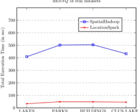
LAKES PARKS BUILDINGS CLUS LAKES 0 100 200 300 400 500 600 700 T otal Execution Time (in sec) RkNNQof real datasets SpatialHadoop LocationSpark

Fig. 1. RkNNQ execution times conside-ring different datasets.

Table 1 summarizes the configuration parameters used in our experiments. Default values (in parentheses) are used unless otherwise mentioned. Spatial-Hadoop needs the datasets to be partitioned and indexed before invoking the spatial operations. The times needed for that pre-processing phase are 94 sec for LAKES, 103 sec for P ARKS, 175 sec for BU ILDIN GS and 200 sec for CLU S LAKES. We decided to exclude indexing time of SpatialHadoop (disk-based DSDMS) for the comparison, since this is anindependent operation. Data

3 _{Available athttp://spatialhadoop.cs.umn.edu/datasets.html} 4

Available athttps://github.com/aseldawy/spatialhadoop2

5

are indexed and the index is stored on HDFS and for subsequent spatial que-ries, data and index are already available (this can be considered as an advan-tage of SpatialHadoop). On the other hand, LocationSpark (in-memory-based DSDMS) always partitions and indexes the data for every operation. The parti-tions/indexes are not stored on any persistent file system and cannot be reused in subsequent operations.

Our first experiment aims to measure the scalability of the distributedRkNNQ

algorithms, varying the dataset sizes. As shown in Figure 1, the execution ti-mes in both DSDMSs do not vary too much, showing quite stable performance. This is due to the indexing mechanisms provided by both DSDMSs that allow fast access to only the necessary partitions for the spatial query processing. The smaller execution times shown byLAKES andCLU S LAKESdatasets is due to how the points are distributed into the space and because one dataset is built based on the other, and they show a similar behavior. From the results with real data, we can conclude that LocationSpark is faster for all the datasets (e.g. it is 2131 sec faster for the biggest dataset,CLU S LAKES) thanks to its memory-based processing that allows to reduce execution times considerably.

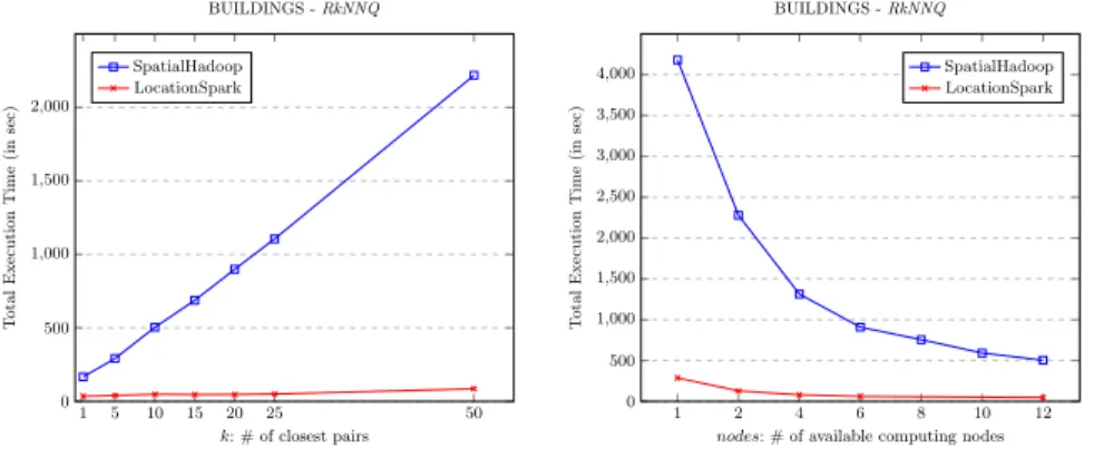
1 5 10 15 20 25 50 0 500 1,000 1,500 2,000 k: # of closest pairs T otal Execution Time (in sec) BUILDINGS -RkNNQ SpatialHadoop LocationSpark 1 2 4 6 8 10 12 0 500 1,000 1,500 2,000 2,500 3,000 3,500 4,000

nodes: # of available computing nodes

T otal Execution Time (in sec) BUILDINGS -RkNNQ SpatialHadoop LocationSpark

Fig. 2.RkNNQ cost (execution time) vs. k values (left). Query cost with respect to the number of computing nodes (nodes) (right).

The second experiment studies the effect of the increasing k value for the largest full-real dataset (BU ILDIN GS). The left chart of Figure 2 shows that the total execution time grows as the value of kincreases. As we can see from the results, the execution time for SpatialHadoop grows much faster than for LocationSpark. This is because as the value ofk increases, so does the number of candidatesK and for each of them a MapReduce job is done. Due to the fact that SpatialHadoop is a disk-based DSDMS, the cost of multiple MapReduce jobs increases the execution time by having to perform different input and output operations for each of the candidate points (for instance, the dataset is read from disk for each candidate). On the other hand, LocationSpark is a in-memory

DSDMS, which allows to reduce the number of disk accesses since the data is already available for each candidate point and thus achieving faster and more stable results even for largek values.

The third experiment aims to measure the speedup of theRkNNQ MapRe-duce algorithms, varying the number of computing nodes (nodes). The right chart of Figure 2 shows the impact of different number of computing nodes on the performance of parallel RkNNQ algorithm, forBU ILDIN GS with the default configuration values. From this chart, it could be concluded that the per-formance of our approach has a direct relationship with the number of computing nodes. It could also be deduced that better performance would be obtained if more computing nodes are added. LocationSpark is still outperforming Spati-alHadoop and it is affected to a lesser degree despite reducing the number of available computing nodes.

By analyzing the previous experimental results, we can extract several con-clusions that are shown below:

– We have experimentally demonstrated theefficiency (in terms of total exe-cution time) and thescalability (in terms ofk values, sizes of datasets and number of computingnodes) of the proposed parallel and distributed algo-rithms forRkNNQ in SpatialHadoop and LocationSpark.

– The larger thekvalues, the greater the number of candidates to be verified, more tasks will be needed and more total execution time is consumed for reporting the final result.

– The larger the number of computingnodes, the faster theRkNNQalgorithms are.

– Both DSDMSs have similar behavior trends, in terms of execution time, although LocationSpark shows better values in all cases (if an adequate number of processing nodes with adequate memory resources are provided), thanks to its in-memory processing performance and capabilities.

5

Conclusions and Future Work

The RkNNQ has received increasing attention in the past years. This spatial query has been actively studied in centralized environments, however, it has not attracted similar attention for parallel and distributed frameworks. For this re-ason, in this paper, we compare two of the most modern and leading DSDMSs, namely SpatialHadoop and LocationSpark. To do this, we have proposed novel algorithms in SpatialHadoop and LocationSpark, the first ones in the literature, to perform efficient parallel and distributed RkNNQ algorithms on big spatial real-world datasets. The execution of a set of experiments has demonstrated that LocationSpark is the overall winner for the execution time, due to the efficiency of memory processing provided by Spark. However, SpatialHadoop shows in-teresting performance trends due to the nature of the proposed algorithm, since the use of multiple MapReduce jobs in a disk-based DSDMS needs multiple disk accesses to datasets. Our current proposal is a good foundation for the develop-ment of further improvedevelop-ments in which the number of candidate points could be

reduced by adapting recentRkNNQ algorithms [16] to MapReduce methodology. Other future work might cover studying other Spark-based DSDMSs likeSimba

[15] and implement other spatial partitioning techniques [3].

References

1. A. Aji, F. Wang, H. Vo, R. Lee, Q. Liu, X. Zhang and J.H. Saltz: “Hadoop-GIS: A high performance spatial data warehousing system over MapReduce”,PVLDB 6(11): 1009-1020, 2013.

2. J. Dean and S. Ghemawat: “MapReduce: Simplified data processing on large clus-ters”,OSDI Conference, pp. 137-150, 2004.

3. A. Eldawy, L. Alarabi and M.F. Mokbel: “Spatial partitioning techniques in Spa-tialHadoop”,PVLDB8(12): 1602-1613, 2015.

4. A. Eldawy and M.F. Mokbel: “SpatialHadoop: A MapReduce framework for spatial data”,ICDE Conference, pp. 1352-1363, 2015.

5. F. Garc´ıa, A. Corral, L. Iribarne, M. Vassilakopoulos and Y. Manolopoulos: “En-hancing SpatialHadoop with Closest Pair Queries”,ADBIS Conference, pp. 212-225, 2016.

6. C. Ji, H. Hu, Y. Xu, Y. Li and W. Qu: “Efficient Multi-dimensional Spatial RkNN Query Processing with MapReduce”,ChinaGrid Conferencepp. 63-68, 2013. 7. C. Ji, W. Qu, Z. Li, Y. Xu, Y. Li and J. Wu: “Scalable multi-dimensional RNN

query processing”,Concurrency and Computation: Practice and Experience27(16): 4156-4171, 2015.

8. F. Korn and S. Muthukrishnan: “Influence Sets Based on Reverse Nearest Neighbor Queries”,SIGMOD Conferencepp. 201-212, 2000.

9. F. Li, B.C. Ooi, M.T. ¨Ozsu and S. Wu: “Distributed data management using MapReduce”,ACM Comput. Surv.46(3): 31:1-31:42, 2014.

10. A. Singh, H. Ferhatosmanoglu and H.S. Tosun: “High Dimensional Reverse Nearest Neighbor Queries”,CIKM Conference, pp. 91-98, 2003.

11. I. Stanoi, D. Agrawal and A. El Abbadi: “Reverse Nearest Neighbor Queries for Dynamic Databases”,SIGMOD Workshop on Research Issues in Data Mining and Knowledge Discovery, pp. 44-53, 2000.

12. M. Tang, Y. Yu, Q.M. Malluhi, M. Ouzzani and W.G. Aref: “LocationSpark: A Distributed In-Memory Data Management System for Big Spatial Data”,PVLDB 9(13): 1565-1568, 2016.

13. Y. Tao, D. Papadias and X. Lian: “Reverse kNN Search in Arbitrary Dimensiona-lity”,VLBD Conference, pp. 744-755, 2004.

14. W. Wu, F. Yang, C.Y. Chan and K.L. Tan: “FINCH: evaluating reverse k-Nearest-Neighbor queries on location data”,PVLDB1(1): 1056-1067, 2008.

15. D. Xie, F. Li, B. Yao, G. Li, L. Zhou and M. Guo: “Simba: Efficient In-Memory Spatial Analytics”,SIGMOD Conference, pp. 1071-1085, 2016.

16. S. Yang, M.A. Cheema, X. Lin and W. Wang: “Reverse k Nearest Neighbors Query Processing: Experiments and Analysis”,PVLDB8(5): 605-616, 2015.

17. M. Zaharia, M. Chowdhury, T. Das, A. Dave, J. Ma, M. McCauly, M.J. Franklin, S. Shenker and I. Stoica: “Resilient Distributed Datasets: A Fault-Tolerant Ab-straction for In-Memory Cluster Computing”,NSDI Conference, pp. 15-28, 2012. 18. H. Zhang, G. Chen, B.C. Ooi, K.-L. Tan and M. Zhang: “In-Memory Big Data