Orthonormal Basis and Radial Basis Functions in Modeling and Identification of Nonlinear Block-Oriented Systems

Selection of our books indexed in the Book Citation Index in Web of Science™ Core Collection (BKCI)

Interested in publishing with us?

Contact [email protected]

Numbers displayed above are based on latest data collected. For more information visit www.intechopen.com Open access books available

Countries delivered to _{Contributors from top 500 universities} International authors and editors

Our authors are among the

most cited scientists

Downloads

We are IntechOpen,

the world’s leading publisher of

Open Access books

Built by scientists, for scientists

12.2%

122,000

135M

TOP 1%

154

16

Orthonormal Basis and Radial Basis Functions

in Modeling and Identification of Nonlinear

Block-Oriented Systems

Rafa

ł

Stanis

ł

awski and Krzysztof J. Latawiec

Department of Electrical, Control and Computer Engineering

Opole University of Technology

Poland

1. Introduction

Nonlinear block-oriented systems, including the Hammerstein, Wiener and feedback-nonlinear systems have attracted considerable research interest both from the industrial and academic environments (Bai, 1998), (Greblicki, 1989), (Latawiec, 2004), (Latawiec et al., 2003), (Latawiec et al., 2004), (Pearson & Pottman, 2000).

It is well known that orthonormal basis functions (OBF) (Bokor et al., 1999) have proved to be useful in identification and control of dynamical systems, including nonlinear block-oriented systems (Gómez & Baeyens, 2004), (Latawiec, 2004), (Latawiec et al., 2003), (Latawiec et al., 2006), (Latawiec et al., 2004), (Stanisławski et al., 2006). In particular, an inverse OBF (IOBF) modeling approach has been effective in identification of a linear dynamic part of the feedback-nonlinear and Hammerstein systems (Latawiec, 2004), (Latawiec et al., 2004). On the other hand, regular OBF (ROBF) modeling approach has proved to be useful in identification of the Wiener system. The approaches provide the separability in estimation of linear and nonlinear submodels (Latawiec et al., 2004), thus eliminating the bilinearity issue detrimentally affecting e.g. the ARX-based modeling schemes (Latawiec, 2004), (Latawiec et al., 2003), (Latawiec et al., 2006), (Latawiec et al., 2004). The IOBF modeling approach is continued to be efficiently used here to model a linear dynamic part of the feedback-nonlinear and Hammerstein systems and regular OBF modeling approach is used to model a linear part of the Wiener system.

The problem of modeling of a nonlinear static part of the nonlinear block-oriented system can be classically tackled using e.g. the polynomial expansion (Latawiec, 2004), (Latawiec et al., 2004) or (cubic) spline functions. Recently, a radial basis function network (RBFN) has been used to model a nonlinear static part of the Hammerstein and feedback-nonlinear systems and a very good identification performance has been obtained (Hachino et al., 2004), (Stanisławski, 2007), (Stanisławski et al., 2007). The concept is extended here to cover the Wiener system.

This paper presents a new strategy for nonlinear block-oriented system identification, which is a combination of OBF modeling for a linear dynamic part and RBFN modeling for a nonlinear static element. The effective OBF approach is finally coupled with the RBFN modeling concept, giving rise to the introduction of a powerful method for identification of the nonlinear block-oriented system.

2. Regular and inverse OBF modelling concept

2.1 Regular OBF modeling

It is well known that an open-loop stable linear discrete-time system described by the transfer function G(q) can be represented with an arbitrary accuracy by the model

∑

=

= M i ciLi q q

Gˆ( ) ₁ ( ), including a series of orthonormal transfer functions Li(q) and the

weighting parameters ci, i=1,...,M, characterizing the model dynamics. Thus, the model of

the system can be written as (Latawiec, 2004), (Latawiec et al., 2006), (Latawiec et al., 2004)

∑

= = M i i iL q ut c t y 1 ) ( ) ( ) ( ˆ (1)

Various OBF can be used in (1). Two commonly used sets of OBF are simple Laguerre and Kautz functions. These functions are characterized by the ‘dominant’ dynamics of a system, which is given by a single real pole (p) or a pair of complex ones (p, p*), respectively.

In case of discrete Laguerre models to be exploited hereinafter, the orthonormal functions

1 2 1 1 ) , ( − ⎥ ⎦ ⎤ ⎢ ⎣ ⎡ − − − − = i i p q pq p q p p q L i=1,...,M (2)

consist of a first-order low-pass factor and (i-1)th-order all-pass filters. Dominant Laguerre pole p can be selected in an experimental way or can be determined with the aid of the stochastic gradient (SG) estimator (Boukis et al., 2006), (Oliveira, 2000).

2.1 Inverse OBF modeling

In case of use of the inverse OBF (IOBF) concept to model a linear dynamic part, the model equation can be presented in form

) ( ) ( ˆ ) ( ˆ 1 _{q yt ut} G− = (3a) ) ( ) ( ˆ ) (q y t u t R = (3b)

where FIR model R(q)= 1 1 1 1 1 1 0 ... ... + + − − − + − _{+ + + +} + L d L d d d d _{r q r r q r q} q

r is the inverse of the system model Gˆ(

q

). In the IOBF concept, the inverse R(q) of the system is modeled using OBF. An OBF modeling approach can now be applied to equation (3b) instead of (3a) and finally we can present equation (1) in the following form (Latawiec et al., 2003)

( )

( , )

( )

0 ( ) 1( ) 1 t e d t u t y p q L c y i M i i

t

+

∑

= − + = β (4)

where e1(t) is the equation error, d is the time delay of the system, β0 and ci i=1,…,M are the

OBF model parameters.

3. RBF network

The nonlinear function approximated by a Radial Basis Functions Network (RBFN) consists of two layers of neurons (one hidden and one output layer). The hidden layer consists of m

Orthonormal Basis and Radial Basis Functions in Modeling and Identification

of Nonlinear Block-Oriented Systems 279

neurons, where each neuron implements the radial activated function. The output layer consists of one linear neuron which realizes weighted sum of outputs of hidden layer neurons. The output of RBFN is described by the equation

))( ( 1 ) ( ut i i w t x _i m φ

∑

= = (5)

where wi, i=1,…,m are the weighting coefficients and φi(u(t)) are the outputs of hidden layer

neurons. Typically, the Gaussian function is used as an activation function in RBFN. The Gaussian functions are modeled by two parameters characterizing their centers αi and wides σi. In this case the φi(u(t)) is given by the equation

(

2 2

)

/ ) ( exp )) ( ( i i i u t u k α σ φ = − − for i=1,..,m (6) where ||.|| is the Euclidian norm.

Important advantage of the RBF network is that the weighting coefficients wi, i=1,…,m can

by estimated by using classical, linear estimation schemes e.g. recursive/adaptive least squares (RLS/ALS), or least mean squares (LMS). The centers αi and wides σi (i=1,…,m) of

the RBF can be determined with the aid of the stochastic gradient (SG) estimator (Kim et al., 2006), genetic algorithm (Hachino et al., 2004) or other optimization methods. However, in practical applications, the optimization of the αi and σi is not absolutely necessary. It has

been found in simulations (Stanisławski, 2007) that RBFN without optimization (with regular distribution of the centers and constant widths) can produce satisfactory solutions.

3. Nonlinear block-oriented systems

3.1 Hammerstein system

The Hammerstein system consists of two cascaded elements, where the first one is a nonlinear memoryless gain and the second one is a linear dynamic model. The whole Hammerstein system can be described by the equation

[

( ( )) ( )

]

( )

[

( ) ( )

]

) ( ) (t G q f u t e t G q xt e t y = + _H = + _H (7)

where G(q) models a dynamic linear part, f(.) describes a nonlinear function, x(t) is the unmeasured output of the nonlinear part and eH(t) is the error/disturbance term. An

alternative output error/disturbance formulation is also possible.

Combining equations (4),(5) and (7) we arrive at the equation describing the whole Hammerstein system

( )

( )

( ( )) ( ) 1 ) , ( _{0 1} 1 t e d t u i i w t y p q L c y M _i m _i i i

t

− + = = +

∑

∑

= φ β (8)

Assuming that wj=β0wj, i=1…m, the model output from the Hammerstein system can be

finally given as

∑

∑

= = − + − = m j j j M i i iL q p y t w t d c 1 1 ) ( ) ( ) , ( ( ˆ t) φ y (9)

θ ϕ

(

)

)

(

ˆ

t

t

y

= T (10) where ϕT(t) =[-v1(t) ... -vM(t) φ1(t-d) φ2(t-d)... φm(t-d)], θ =[c1 ... cM w1 w2 ... wm] and vi(t)=Li(q,p)y(t). Unknown parameters θ of the model can be estimated by the familiar

recursive least squares (RLS) or least mean squares (LMS) algorithms.

3.2 Wiener system

In a single-input single-output Wiener system, a linear dynamic part is cascaded with a nonlinear static element. The output yˆ(t) of the Wiener model, or the system output predictor, can be calculated as

(q)u(t)] G [ f (t) yˆ = ˆ ˆ (11)

Since a nonlinear static characteristic is invertible we can rewrite equation (11) in form

) ( ) (q u t G t y fˆ−1[ˆ( )]= ˆ (12) The function ˆ 1[ˆ( )] t y

f− can be approximated with RBF network. Finally, we arrive at the linear regression function

)) ( ( ) ( ) ( ( ˆ 1 1 1 _{y t} i w t u q L c _i m i M i i i

∑

φ

∑

= = − ₋ = ) t y (13)

where w_i =w_i−α_i (i=1,..,m), which can be presented in the familiar form

y

ˆ

(

t

)

=ϕT

(

t

)

θ

, with ϕT(t)

= [ v1(t) ... -vM(t) -φ1(y(t)) -φ2(y(t))... -φm(y(t))], θ=[c1 ... cM w1 w2 ... wm] and vi(t)=Li(q,p)u(t), i=1,...,M.

3.3 Feedback-nonlinear system

In the block-oriented feedback-nonlinear system, the output of the linear dynamic part is fed (negatively) back to the input through the static nonlinearity, so that the whole system can be described by the equation

[

]

[

( ) ( ) ( )

]

) ( ) ( )) ( ( ) ( ) ( ) ( t e t x t u q G t e t y f t u q G t y F F + − = + − = (14)

where eF(t) is the error/disturbance term. Combining equations (4),(5) and (14) we arrive at

the equation describing the whole, IOBF-related feedback-nonlinear system (Stanisławski et al., 2007)

( )

( )

( ( )) ( ) 1 ) ( ) , ( ₀ 1 t e d t y j j w d t u t y p q L c y M _i m _j i i

t

+ ⎥ ⎥ ⎦ ⎤ ⎢ ⎢ ⎣ ⎡ − = − − = +

∑

∑

= φ β (15)

Putting wj=β0wj, j=1…m, the output from the feedback-nonlinear system can be finally given

Orthonormal Basis and Radial Basis Functions in Modeling and Identification

of Nonlinear Block-Oriented Systems 281

( )

( )

( ( )) ( ) 1 ) , ( ) ( 1 0 y t d et j j w t y p q L c d t u y _j m i M i i

t

− + = − − − =

∑

∑

= φ β (16)

The equation (16) can be presented in the linear regression form, with ϕT(t)

=[u(t-d) -v1(t) ...

-vM(t) -φ1(y(t-d)) -φ2(y(t-d))... -φm(y(t-d))], θ=[β0 c1 ... cM w1 w2 ... wm] and vi(t)=Li(q,p)y(t).

Clearly, owing to the IOBF modeling approach applied, the linear and nonlinear submodels are separated from each other so that the bilinearity issue is eliminated here.

4. Simlation experiments

In the Matlab/Simulink environment, we comparatively analyze the three presented nonlinear block-oriented OBF/RBFN-related models consisting of 1) Hammerstein IOBF related model, 2) Wiener regular OBF related model and 3) feedback-nonlinear IOBF related model. For example, consider the magnetic levitation process which has been simulated as a demo in the Matlab/Simulink environment. Our main goal is to analyze efficiency of the approach in view of their possible use in on-line identification (and control). Performance of parameter estimation is evaluated by means of the mean square prediction error (MSPE). MSPE is described by the equation

∑

= − = N t t y t y N MSPE 1 2 )) ( ˆ ) ( ( ) 1 ( (17)

The system is excited by a random number generator with regular distribution <0.5, 4>. Additionally, the system is corrupted with the input and output noises (ei(t) and eo(t)), which

are supplied from a Gaussian random number generators with N(0, δi) and N(0, δo),

respectively. For estimation of weights of the RBFs and parameters of the dynamical model we use a classical RLS algorithm.

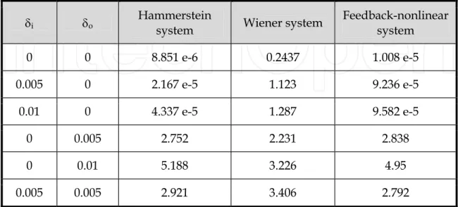
Table 1 specifies the results of a comparative analysis of the performance of the three models for M=6 and m=9.

δi δo Hammerstein

system Wiener system

Feedback-nonlinear system 0 0 8.851 e-6 0.2437 1.008 e-5 0.005 0 2.167 e-5 1.123 9.236 e-5 0.01 0 4.337 e-5 1.287 9.582 e-5 0 0.005 2.752 2.231 2.838 0 0.01 5.188 3.226 4.95 0.005 0.005 2.921 3.406 2.792 Table 1. MSPE of the Hammerstein, Wiener and feedback-nonlinear models

The results in Table 1 show that the high accuracy of identification has been obtained for the IOBF/RBFN-based models (Hammerstein and feedback-nonlinear models). The reasons are 1) the specific, structure of the IOBF-related model, 2) numerical conditioning of the covariance matrix for the IOBF-based estimation problem is essentially better than that for the OBF-based one. However, the inconvenience of IOBF-related models is the high sensitivity on the output error due to the equation error structure. Table 1 shows that the Wiener model cannot provide sufficiently high accuracy of the identification problem, causing that the RBF network in the Wiener system models the inversion of the nonlinear function f(.). The calculation of the original function on the basis of RBF network is ambiguous and badly numerical conditioned. Finally, only the Wiener model gives the satisfy results for the system corrupted with the high-level disturbances.

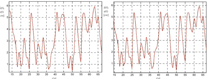
Plots of the actual output and its reconstruction by Hammerstein, Wiener and Feedback nonlinear models presented in Fig. 1 and Fig. 2 confirm very good performance of identification for Hammerstein and Feedback nonlinear models and poor performance for Wiener model, respectively.

15 20 25 30 35 40 45 50 55 60 65 1 2 3 4 5 6 t [s] ] [ ) ( ), ( ˆ cm t y t y 15 20 25 30 35 40 45 50 55 60 65 1 2 3 4 5 6 ] [ ) ( ), ( ˆ cm t y t y t [s]

Fig. 1. Plots of actual (solid-black) vs. predicted (dashed-red) outputs of the Hammerstein system (left) and feedback-nonlinear system (right)

] [ ) ( ), ( ˆ cm t y t y t [s] 15 20 25 30 35 40 45 50 55 60 65 1 2 3 4 5 6

Orthonormal Basis and Radial Basis Functions in Modeling and Identification

of Nonlinear Block-Oriented Systems 283

7. Conclusion

The paper has presented the solutions to the nonlinear identification problem for the various nonlinear block-oriented systems using OBF-related models and RBF network. We have demonstrated that the Wiener model based on regular OBF modeling concept cannot provide sufficiently high performance of the identification problem. This is mainly to due with inversion problem of RBF network.

Results of a simulation analysis have shown that the strategy using the IOBF modeling concept in Hammerstein and feedback-nonlinear model can provide a very good performance, both in terms of low prediction errors and accurate reconstruction of the nonlinear characteristics, in addition to high computational efficiency.

8. References

Bai E.W. (1998). An optimal two-stage identification algorithm for Hammerstein-Wiener nonlinear systems. Automatica, Vol. 34, pp. 333-338.

Bokor J., Heuberger P., Ninness, B., Oliveira e Silva, T., Van den Hof P. & Wahlberg, B. (1999). Modelling and identification with orthogonal basis functions. Proc. Preconference Workshop, 14th _{IFAC World Congress, Beijing, P.R. China.}

Boukis C., Mandic D.P., Constantinides A.G. & Polymenakos L.C. (2006). A Novel Algorithm for the Adaptation of the Pole of Laguerre Filters. IEEE Signal Processing Letters, Vol. 13, No. 7, pp. 429 - 432.

Greblicki W. (1989). Nonparametric orthogonal series identification of Hammerstein systems. International Journal of Systems Science, Vol. 20, No. 12, pp. 2355-2367.

Gómez J.C. & Baeyens E. (2004). Identification of block-oriented nonlinear systems using orthonormal bases. Journal of Process Control, Vol. 14, No. 6, pp. 685-697

Hachino T., Deguchi K. & Takata H. (2004). Identification of Hammerstein model using radial basis function networks and genetic algorithm. Proc. 5th Asian Control Conference, Vol. 1, pp. 124-129.

Kim N.Y., Byun H.G. & Kwon K.H. (2006). Learning Behaviors of Stochastic Gradient Radial Basis Function Network Algorithms for Odor Sensing Systems. ETRI journal, Vol. 28, No. 1.

Latawiec K.J. (2004) The Power of Inverse Systems in Modeling and Control of Linear and Nonlinear Systems. Vol. 167, Opole University of Technology Press, Opole, Poland. Latawiec K.J., Marciak C., Hunek W. & Stanisławski R. (2003) A new analytical design

methodology for adaptive control of nonlinear block-oriented systems. Proc. 7th World Multi-Conference on Systemics, Cybernetics and Informatics, Vol. XI, pp. 215-220, Orlando, Florida, USA.

Latawiec K.J., Marciak C. & Oliveira G.H.C.: (2006). A new control-oriented modeling methodology for a series DC motor. Electromagnetic Fields in Mechatronics, Electrical and Electronic Engineering, Wiak S., Krawczyk A. & Fernandez X.L.M. (Eds.), IOS Press, Studies in Applied Electromagnetics and Mechanics, Vol. 27, Chapter_B_13. Latawiec K.J., Marciak C., Rojek R. & Oliveira G.H.C. (2003). Linear parameter estimation

and predictive constrained control of Wiener/Hammerstein systems. Proc. 13th IFAC Symposium on System Identification, pp. 359-364, Rotterdam, The Netherlands.

Latawiec K.J., Marciak C., Stanisławski R. & Oliveira G.H.C. (2004) The mode separability principle in modeling of linear and nonlinear blockoriented systems. Proc. the 10th

IEEE MMAR Conference (MMAR’04), Vol. 1, pp. 479-484, Miedzyzdroje, Poland.

Oliveira S.T. (2000). Optimal pole conditions for Laguerre and two-parameter Kautz models: a survey of known results. Proc. 12th IFAC Symp. on System Identification (SYSID'2000), pp. 457-462, Santa Barbara, CA, USA.

Pearson R.K. & Pottman M. (2000). Gray-box identification of block-oriented nonlinear models. Journal of Process Control, Vol. 10, pp. 301-315.

Stanisławski R., Latawiec K.J. & Stanisławski W. (2006). Modeling of a boiler proper using a complex structure model by means of multivariable orthonormal basis functions.

Proc. 12th IEEE MMAR Conference (MMAR’06), pp. 935-938, Miedzyzdroje, Poland.

Stanisławski R. (2007). Hammerstein system identification by means of orthonormal basis functions and radial basis functions. Emerging Technologies, Robotics and Control Systems, Pennacchio S. (Eds.), Internationalsar, Vol. 2, pp. 69-73, Palermo, Italy. Stanisławski R., Latawiec K.J. & Hunek W.P. (2007). Identification of feedback-nonlinear

systems by means of orthonormal basis and radial basis functions. Proc. 13th IEEE

Automation and Robotics

Edited by Juan Manuel Ramos Arreguin

ISBN 978-3-902613-41-7 Hard cover, 388 pages

Publisher I-Tech Education and Publishing

Published online 01, May, 2008

Published in print edition May, 2008

InTech Europe

University Campus STeP Ri Slavka Krautzeka 83/A 51000 Rijeka, Croatia Phone: +385 (51) 770 447 Fax: +385 (51) 686 166 www.intechopen.com

InTech China

Unit 405, Office Block, Hotel Equatorial Shanghai No.65, Yan An Road (West), Shanghai, 200040, China Phone: +86-21-62489820

Fax: +86-21-62489821

In this book, a set of relevant, updated and selected papers in the field of automation and robotics are presented. These papers describe projects where topics of artificial intelligence, modeling and simulation process, target tracking algorithms, kinematic constraints of the closed loops, non-linear control, are used in advanced and recent research.

How to reference

In order to correctly reference this scholarly work, feel free to copy and paste the following:

Rafal Stanislawski and Krzysztof J. Latawiec (2008). Orthonormal Basis and Radial Basis Functions in Modeling and Identification of Nonlinear Block-Oriented Systems, Automation and Robotics, Juan Manuel Ramos Arreguin (Ed.), ISBN: 978-3-902613-41-7, InTech, Available from:

http://www.intechopen.com/books/automation_and_robotics/orthonormal_basis_and_radial_basis_functions__i n_modeling_and_identification_of_nonlinear__block-ori

under the terms of the

Creative Commons

Attribution-NonCommercial-ShareAlike-3.0 License

, which permits use, distribution and reproduction for

non-commercial purposes, provided the original is properly cited and

derivative works building on this content are distributed under the same

license.