regression problems
Emilio Seijo
Submitted in partial fulfillment of the requirements for the degree
of Doctor of Philosophy
in the Graduate School of Arts and Sciences
COLUMBIA UNIVERSITY
Emilio Seijo All Rights Reserved
Statistical inference in two non-standard
regression problems
Emilio Seijo
This thesis analyzes two regression models in which their respective least squares estimators have nonstandard asymptotics. It is divided in an intro-duction and two parts. The introintro-duction motivates the study of nonstandard problems and presents an outline of the contents of the remaining chapters. In part I, the least squares estimator of a multivariate convex regression func-tion is studied in great detail. The main contribufunc-tion here is a proof of the consistency of the aforementioned estimator in a completely nonparametric setting. Model misspecification, local rates of convergence and multidimen-sional regression models mixing convexity and componentwise monotonicity constraints will also be considered. Part II deals with change-point regres-sion models and the issues that might arise when applying the bootstrap to these problems. The classical bootstrap is shown to be inconsistent on a sim-ple change-point regression model, and an alternative (smoothed) bootstrap procedure is proposed and proved to be consistent. The superiority of the al-ternative method is also illustrated through a simulation study. In addition, a
List of Figures vi
Acknowledgments vii
Chapter 1 Introduction 1
I
Convex Regression
6
Chapter 2 Multivariate Convex Regression 7
2.1 Least squares estimation of a multivariate convex regression
function . . . 7
2.2 Characterization and finite sample properties. . . 12
2.2.1 Existence and uniqueness . . . 13
2.2.2 Finite sample properties . . . 16
2.2.3 Computation of the estimator . . . 17
2.3 Consistency of the least squares estimator . . . 19
2.3.1 Fixed Design . . . 21
2.3.2 Stochastic Design . . . 22
2.3.3 Main results . . . 23
2.3.4 Proof of the main results . . . 24
2.4 Proofs of auxiliary lemmas . . . 30 i
2.4.2 Proof of Lemma 2.3.2. . . 35 2.4.3 Proof of Lemma 2.3.3. . . 39 2.4.4 Proof of Lemma 2.3.4. . . 39 2.4.5 Proof of Lemma 2.3.5. . . 41 2.4.6 Proof of Lemma 2.3.6. . . 44 2.4.7 Proof of Lemma 2.3.7. . . 44 2.4.8 Proof of Lemma 2.3.8. . . 48 2.4.9 Proof of Lemma 2.3.9. . . 50 2.4.10 Proof of Lemma 2.3.10 . . . 51
Chapter 3 Additional topics regarding convex regression 53 3.1 The one-dimensional case. . . 53
3.2 Convex and componentwise monotone regression functions . . 54
3.2.1 The convex, α-monotone least squares estimator: com-putation and finite sample properties . . . 55
3.2.2 The convex, α-monotone least squares estimator: con-sistency . . . 58
3.3 Behavior under misspecified model . . . 58
3.4 A conjecture about local rates of convergence . . . 60
3.4.1 Some further notation and assumptions . . . 61
3.4.2 On the measurability of subdifferentials and subgradients 62 3.4.3 The conjecture and the ideas behind it . . . 62
II
Change-point Regression
72
Chapter 4 A continuous mapping theorem for the smallest argmax
functional 73
4.2 The Skorohod spaceDK . . . 76
4.2.1 Definition and basic properties. . . 76
4.2.2 The Skorohod topology . . . 79
4.2.3 The sargmax functional on DK . . . 83
4.3 A continuous mapping theorem for the sargmax functional on functions with jumps . . . 86
4.4 On the necessity of the convergence of the associated pure jump processes . . . 92
4.5 Applications . . . 93
4.5.1 Stochastic design change-point regression . . . 93
4.5.2 Estimation in a Cox regression model with a change-point in time . . . 94
4.5.3 Estimating a change-point in a Cox regression model according to a threshold in a covariate . . . 97
Chapter 5 Change-point regression and the bootstrap 100 5.1 Introduction . . . 100
5.2 The problem and the bootstrap schemes . . . 103
5.2.1 Bootstrap . . . 104
5.3 A uniform convergence result . . . 108
5.3.1 Consistency and the rate of convergence . . . 109
5.3.2 Weak Convergence and asymptotic distribution . . . . 111
5.4 Inconsistency of the bootstrap . . . 116
5.4.1 Scheme 1 (Bootstrapping from ECDF) . . . 117
5.4.2 Scheme 2 (Bootstrapping “residuals”) . . . 124
5.5 Consistent bootstrap procedures . . . 126
5.5.1 Scheme 3 (Smoothed Bootstrap). . . 127 iii
5.6 Simulation experiments . . . 128
5.7 More general change-point regression models . . . 131
5.8 Acknowledgement . . . 134 5.9 Supplementary Lemmas . . . 134 5.9.1 Proof of Proposition 5.3.1 . . . 137 5.9.2 Proof of Proposition 5.3.2 . . . 139 5.9.3 Proof of Lemma 5.3.1. . . 142 5.9.4 Proof of Lemma 5.3.2. . . 143 5.9.5 Proof of Lemma 5.3.3. . . 145 5.9.6 Proof of Lemma 5.3.4. . . 149 5.9.7 Proof of Proposition 5.3.3 . . . 149 5.9.8 Proof of Lemma 5.4.1. . . 150 5.9.9 Proof of Lemma 5.4.2. . . 151 5.9.10 Proof of Lemma 5.4.4. . . 154 5.9.11 Proof of Lemma 5.4.6. . . 157 5.9.12 Proof of Lemma 5.4.7. . . 160 5.9.13 Proof of Proposition 5.4.2 . . . 161 5.9.14 Proof of Lemma 5.4.8. . . 163 5.9.15 Proof of Proposition 5.5.1 . . . 164 5.9.16 Proof of Proposition 5.5.2 . . . 165 5.9.17 Proof of Proposition 5.5.3 . . . 166 iv
Appendix
184
Appendix A Convex analysis 184
A.1 Polar coordinates based on boundaries of convex sets . . . 186 A.2 Restrictions of convex functions to compact, convex subsets of
their effective domains . . . 189
Appendix B Results from linear algebra 194
B.1 Proof of Lemma 2.4.1 . . . 195 B.2 Proof of Lemma 2.4.2 . . . 198 B.3 Proof of Lemma 2.4.3 . . . 201
2.1 The scatter plot and nonparametric least squares estimator of the convex regression function when (a)φ(x) = |x|2(left panel);
(b) φ(x) = −x1+x2 (right panel). . . . . 19
2.2 Explanatory diagram for (a) Lemma 2.4.1 (left panel); (b) Lemma 2.4.2 (right panel). . . 33 2.3 Explanatory diagram for (a) Lemma 2.4.3 (left panel); (b)
Lemma 2.3.2 (right panel). . . 34 2.4 The smallest distance between∂Kzand∂Xis at least
rmin1≤j≤d{bj−aj}
2|b−a| . 41
5.1 Histograms of the distribution of n(ˆζn−ζ0) and its bootstrap
estimates: the asymptotic distribution of n(ˆζn−ζ0) (top left);
the actual distribution ofn(ˆζn−ζ0) (top middle); the
distribu-tion ofn(ζn∗−ζˆn) for the smoothed (top right), ECDF (bottom
middle) and FDR (bottom right) schemes; the distribution of
mn(ζn∗−ζˆn),mn =dn
4
5e (bottom left). . . 132
I want to take this opportunity to express my most sincere gratitude to my advisor, professor Bodhisattva Sen. It would have been impossible for me to complete this thesis without his patience, guidance and direction. It was a privilege to work closely with someone who enjoys statistical inference as much as he does. I would also like to acknowledge all my professors at Columbia from whom I learned so much. I am particularly grateful to professors Richard Davis, Zhiliang Ying, David Madigan and Jos´e Blanchet. The advice they gave me at different stages during the completion of the Ph.D. program were very helpful and enlightening. In addition, I would like to thank my disserta-tion committee: Professor Richard Davis, professor Ian McKeague, professor Jos’´e Blanchet, professor Zhiliang Ying, and professor Bodhisattva Sen. I truly appreciate the time they took to read through my work.
I am also grateful to all my classmates and friends at Columbia. I would like to acknowledge all the help that I received, especially during my first couple of years in the Ph.D. program, from Tyler McCormick, Subhankar Sadhukan, Johannes Ruf and Gerardo Hern´andez del Valle. My discussions with them were always illustrative and taught me a lot about probability, statistics and programming. I also want to recognize the work of all the staff
were an integral part of my success at Columbia.
I am thankful to professor Moulinath Banerjee, from the University of Michigan, and Souvik Gosh. Their help was essential for the completion of this work.
Last but not least, I want to thank my family and friends for all their support. I am particularly grateful to my parents and Alejandra, for their ever present support and advice.
Chapter 1
Introduction
This dissertation comprises the statistical analysis of two regression models. The first of these is a regression problem in which the regressand is a convex function of a possibly multidimensional regressor. The other one is the so-called change-point regression problem, and it consists in estimating a jump discontinuity (change-point) in an otherwise smooth curve. Though quite different in nature, these problems share a common characteristic: both can be solved with least squares estimation procedures which exhibit nonstandard asymptotics.
A sequence of consistent estimators in a point estimation problem is said to have nonstandard asymptotics if the estimators converge to a non-Gaussian limiting distribution at a rate other than n−1/2. A trivial example
arises in the estimation ofθ >0 given a random sample from aU nif orm(0, θ) distribution. In this case, the maximum likelihood estimator (MLE), which is the maximum of the sample, converges at rate n−1 to an Exponential(θ−1)
distribution. This problem does not satisfy the regularity conditions that are usually assumed for MLE’s (see eitherLehmann and Casella(1998) orvan der Vaart(1998)). Thus, the standard asymptotic theory of the parametric MLE
does not apply and the result has to be deduced via direct calculations. De-spite its simplicity, this problem illustrates the fact that nonstandard problems require specially tailored solutions.
Nonstandard problems are frequently encountered outside the realm of parametric statistical inference and some of them have been carefully studied in the literature. For instance, Kim and Pollard (1990) show a family of cube-root asymptotic problems arising from a wide array of applications while
Groeneboom et al.(2001) prove that the univariate least squares estimator in convex regression exhibits nonstandard asymptotics (see Section 3.1) In this context, this thesis presents an illustration of the issues that might arise in nonstandard problems and the techniques that can be used to deal with them. The first part of the thesis deals with multidimensional convex regres-sion. This problem involves the estimation of a function with a multidimen-sional argument subject to a shape-restriction (convexity). We will define the least squares estimator in multiple dimensions, provide means for its compu-tations, describe its finite sample properties and prove its strong consistency (and that of its subdifferentials). This is one of the main contributions of this thesis as it constitutes the first attempt to solve this problem in a completely nonparametric setting.
In addition to the consistency of the least squares estimator in multidi-mensional convex regression, we will treat some other topics regarding convex function estimation. In Section 3.1 we describe the complete local asymp-totic theory in the one-dimensional case, illustrating that convex regression is a nonstandard problem. In Section 3.2 we will generalize the methods of Chapter 2to the case in which the regression function is known to be convex and monotone in some subset of the coordinates of its argument. We will argue that the least squares estimator is also consistent in this situation. In
Section 3.3 we will describe some results regarding the behavior of the least squares estimators under misspecified models. We will finish the first part of the thesis by providing a conjecture about local rates of convergence for the least squares estimator in the regular stochastic design convex regression model in dimensions 2 and 3. Besides the conjecture itself, the methods used in this section might be of independent interest. We will define a family of “localizing” functions that can be used to analyze the local properties of the least squares estimator. To the best of our knowledge, this thesis represents the first attempt to achieve this in a multidimensional scenario.
In change-point regression problems one tries to estimate a jump-discontinuity in an otherwise smooth function given a finite random sample. Change-point estimators tend to have the following characteristics: they con-verge at rate n−1; their asymptotic theory is related to two-sided compound processes rather than to Gaussian processes; their limiting distributions have too many nuisance parameters, some of them living in infinite-dimensional spaces; despite being M-estimators, their asymptotic law cannot be deduced from the classical argmax continuous mapping theorem; the classical boot-strap yields inconsistent confidence intervals (for the concept of consistent bootstrap procedures, see Section 5.2.1). The second part of this document will illustrate all these properties of change-point problems and show ways to deal with them.
As mentioned in the previous paragraph, one of the peculiarities of change-point estimators is that they can usually be cast as M-estimators, but the traditional argmax continuous mapping theorem (see Theorem 3.2.2 in page 286 of van der Vaart and Wellner(1996)) cannot be used to derive their limiting laws. This happens because, in the limit, they are maximizers of two-sided compound Poisson processes which have multiple maximizers, almost
surely. To remedy this situation, we force change-point estimators to be the smallest maximizers of their respective objective functions and then prove a version of the continuous mapping theorem pertinent to the situation. We carry this task in Chapter4and provide some examples in which the theorem can be applied.
Other relevant properties of change-point problems are that their limit-ing distributions depend on many nuisance parameters and that the classical bootstrap yields inconsistent confidence intervals. As the classical bootstrap is one of the most popular inferential techniques that avoid dealing with nui-sance parameters, we carefully analyze this situation in Chapter5. The failure of the classical bootstrap in nonstandard problems has been documented in several instances. For example, Bose and Chatterjee (2001), Abrevaya and Huang (2005) and Sen et al. (2010) have documented failure of the classical bootstrap in nonstandard, M-estimation problems (the former) and cube-root asymptotic problems (the latter 2). In Section 5.4 we will argue that the two most common bootstrap methods used in regression problems are inconsistent in the simplest change-point regression problem. Subsequently, two consistent methods for this problem will be provided in Section 5.5. While doing this, we will prove a consistency theorem for triangular arrays of random variables that might be of independent interest (see Proposition5.3.3).
There are two main contributions of the analyses carried out in Chap-ters 4 and 5. On the one hand, the continuous mapping theorem of Chapter 4 is a convergence result that can be applied to many situations involving estimation of jump-discontinuities (see Li and Ling (2012) for an application in the context of threshold autoregressive models). On the other hand, the analysis of the consistency of the bootstrap schemes in Chapter 5 illustrates that the classical bootstrap cannot be trusted in change-point problems (as it
fails in the simplest of such problems), but that smoothed bootstrap schemes are a consistent, easy-to-implement alternative. In addition, this work pro-vides another instance of the inconsistency of the classical bootstrap in a nonstandard situation.
Convex Regression
Chapter 2
Multivariate Convex Regression
2.1
Least squares estimation of a multivariate
convex regression function
Consider a closed, convex setX⊂Rd, for d≥1, with nonempty interior and
a regression model of the form
Y =φ(X) + (2.1)
whereX is aX-valued random vector,is a random variable withE(|X) = 0, and φ : Rd →
R is an unknown convex function. Given independent observations (X1, Y1), . . . ,(Xn, Yn) from such a model, we wish to estimate φ
by the method of least squares, i.e., by finding a convex function ˆφn which
minimizes the discrete L2 norm n
X
k=1
|Yk−ψ(Xk)|2
!12
among all convex functions ψ defined on the convex hull of X1, . . . , Xn. In
this paper we characterize the least squares estimator, provide means for its computation, study its finite sample properties and prove its consistency.
The problem just described is a nonparametric regression problem with known shape restriction (convexity). Such problems have a long history in the statistical literature with seminal papers like Brunk (1955), Grenander
(1956) and Hildreth (1954) written more than 50 years ago, albeit in sim-pler settings. The former two papers deal with the estimation of monotone functions while the latter discusses least squares estimation of a concave func-tion whose domain is a subset of the real line. Since then, many results on different nonparametric shape restricted regression problems have been pub-lished. For instance, Brunk (1970) and, more recently, Zhang (2002) have enriched the literature concerning isotonic regression. In the particular case of convex regression, Hanson and Pledger (1976) proved the consistency of the least squares estimator introduced in Hildreth (1954). Some years later,
Mammen(1991) andGroeneboom et al.(2001) derived, respectively, the rate of convergence and asymptotic distribution of this estimator. Some alterna-tive methods of estimation that combine shape restrictions with smoothness assumptions have also been proposed for the one-dimensional case; see, for example, Birke and Dette (2006) where a kernel-based estimator is defined and its asymptotic distribution derived.
Although the asymptotic theory of the one-dimensional convex regres-sion problem is well understood, not much has been done in the multidimen-sional scenario. The absence of a natural order structure in Rd, for d > 1, poses a natural impediment in such extensions. A convex function on the real line can be characterized as an absolutely continuous function with in-creasing first derivative (see, for instance,Folland(1999), Exercise 42.b, page 109). This characterization plays a key role in the computation and asymp-totic theory of the least squares estimator in the one-dimensional case. By contrast, analogous results for convex functions of several variables involve
more complicated characterizations using either second-order conditions (as in Dudley (1977), Theorem 3.1, page 163) or cyclical monotonicity (as in
Rockafellar (1970), Theorems 24.8 and 24.9, pages 238-239). Interesting dif-ferences between convex functions onRand convex functions onRdare given
inJohansen (1974) and Bron˘ste˘ın (1978).
Recently there has been considerable interest in shape restricted func-tion estimafunc-tion in multidimension. In the density estimafunc-tion context, Cule et al. (2010) deal with the computation of the nonparametric maximum like-lihood estimator of a multidimensional log-concave density, while Cule and Samworth(2010),Schuhmacher et al.(2009) andSchuhmacher and D¨umbgen
(2010) discuss its consistency and related issues. Seregin and Wellner (2009) study the computation and consistency of the maximum likelihood estimator of convex-transformed densities. This paper focuses on estimating a regres-sion function which is known to be convex. To the best of our knowledge this is the first attempt to systematically study the characterization, computation, and consistency of the least squares estimator of a convex regression function with multidimensional covariates in a completely nonparametric setting.
In the field of econometrics some work has been done on this multidi-mensional problem in less general contexts and with more stringent assump-tions. Estimation of concave and/or componentwise nondecreasing functions has been treated, for instance, in Banker and Maindiratta (1992), Matzkin
(1991), Matzkin (1993), Beresteanu (2007) and Allon et al.(2007). The first two papers define maximum likelihood estimators in semiparametric settings. The estimators in Matzkin (1991) and Banker and Maindiratta (1992) are shown to be consistent inMatzkin(1991) andMaindiratta and Sarath(1997), respectively. A maximum likelihood estimator and a sieved least squares es-timator have been defined and techniques for their computation have been
provided in Allon et al. (2007) and Beresteanu (2007), respectively.
The method of least squares has been applied to multidimensional con-cave regression inKuosmanen(2008). We take this work as our starting point. In agreement with the techniques used there, we define a least squares estima-tor which can be computed by solving a quadratic program. We argue that this estimator can be evaluated at a single point by finding the solution to a linear program. We then show that, under some mild regularity conditions, our estimator can be used to consistently estimate both, the convex function and its subdifferentials.
Our work goes beyond those mentioned above in the following ways: Our method does not require any tuning parameter(s), which is a major drawback for most nonparametric regression methods, such as kernel-based procedures. The choice of the tuning parameter(s) is especially problematic in higher dimensions, e.g., kernel based methods would require the choice of a d×d matrix of bandwidths. The sets of assumptions that most authors have used to study the estimation of a multidimensional convex regression function are more restrictive and of a different nature than the ones in this paper. As opposed to the maximum likelihood approach used in Banker and Maindiratta (1992), Matzkin(1991),Allon et al. (2007) and Maindiratta and Sarath (1997), we prove the consistency of the estimator keeping the distri-bution of the errors unspecified; e.g., in the i.i.d. case we only assume that the errors have zero expectation and finite second moment. The estimators in
Beresteanu(2007) are sieved least squares estimators and assume that the ob-served values of the predictors lie on equidistant grids of rectangular domains. By contrast, our estimators are unsieved and our assumptions on the spatial arrangement of the predictor values are much more relaxed. In fact, we prove the consistency of the least squares estimator under both fixed and stochastic
design settings; we also allow for heteroscedastic errors. In addition, we show that the least squares estimator can also be used to approximate the gradients and subdifferentials of the underlying convex function.
It is hard to overstate the importance of convex functions in applied mathematics. For instance, optimization problems with convex objective functions over convex sets appear in many applications. Thus, the question of accurately estimating a convex regression function is indeed interesting from a theoretical perspective. However, it turns out that convex regression is important for numerous reasons besides statistical curiosity. Convexity also appears in many applied sciences. One such field of application is microe-conomic theory. Production functions are often supposed to be concave and componentwise nondecreasing. In this context, concavity reflects decreasing marginal returns. Concavity also plays a role in the theory of rational choice since it is a common assumption for utility functions, on which it represents decreasing marginal utility. The interested reader can see Hildreth (1954),
Varian (1982a) or Varian(1982b) for more information regarding the impor-tance of concavity/convexity in economic theory.
This chapter is organized as follows. In Section 2.2 we discuss the estimation procedure, characterize the estimator and show how it can be computed by solving a positive semidefinite quadratic program and a lin-ear program. Section 2.3 starts with a description of the deterministic and stochastic design regression schemes. The statement and proof of our main results are also included in Section2.3. In Section2.4we provide the proofs of the technical lemmas used to prove the main theorem. The appendix contains some auxiliary results from convex analysis and linear algebra that might be of independent interest.
2.2
Characterization and finite sample
prop-erties
We start with some notation. For convenience, we will regard elements of the Euclidian spaceRm as column vectors and denote their components with up-per indices, i.e, anyz ∈Rm will be denoted asz = (z1, z2, . . . , zm). The
sym-bol R will stand for the extended real line. Additionally, for any set A⊂Rd
we will denoted asConv(A) its convex hull and we’ll writeConv(X1, . . . , Xn)
instead of Conv({X1, . . . , Xn}). Finally, we will use h·,·i and | · | to denote
the standard inner product and norm in Euclidian spaces, respectively. For X = {X1, . . . , Xn} ⊂ X ⊂ Rd, consider the set KX of all vectors
z = (z1, . . . , zn)0 ∈
Rn for which there is a convex function ψ : X → R such that ψ(Xj) = zj for all j = 1, . . . , n. Then, a necessary and sufficient
condition for a convex function ψ to minimize the sum of squared errors is that ψ(Xj) = Znj for j = 1, . . . , n, where
Zn= argmin z∈KX ( n X k=1 Yk−zk 2 ) . (2.2)
The computation of the vector Zn is crucial for the estimation
proce-dure. We will show that such a vector exists and is unique. However, it should be noted that there are many convex functions ψ satisfying ψ(Xj) = Znj for
all j = 1, . . . , n. Although any of these functions can play the role of the least squares estimator, there is one such function which is easily evaluated in Conv(X1, . . . , Xn). For computational convenience, we will define our least
squares estimator ˆφnto be precisely this function and describe it explicitly in
(2.7) and the subsequent discussion.
In what follows we show that both, the vectorZnand the least squares
will also provide two characterizations of the setKX and show that the vector
Zn can be computed by solving a positive semidefinite quadratic program.
Finally, we will prove that for any x ∈ Conv(X1, . . . , Xn) one can obtain
ˆ
φn(x) by solving a linear program.
2.2.1
Existence and uniqueness
We start with two characterizations of the set KX. The developments here
are similar to those in Allon et al. (2007) and Kuosmanen(2008).
Lemma 2.2.1 (Primal Characterization) Letz = (z1, . . . , zn)∈
Rn. Then, z ∈ KX if and only if for every j = 1, . . . , n, the following holds:
zj = inf ( n X k=1 θkzk : n X k=1 θk = 1, n X k=1 θkXk =Xj, θ≥0, θ ∈Rn ) , (2.3) where the inequality θ ≥0 holds componentwise.
Proof: Define the function g :Rd→
R by g(x) = inf ( n X k=1 θkzk : n X k=1 θk = 1, n X k=1 θkXk=x, θ≥0, θ ∈Rn ) (2.4) where we use the convention that inf(∅) = +∞. By Lemma A.0.6 in the Appendix, g is convex and finite on the Xj’s. Hence, if zj satisfies (2.3) then
zj =g(X
j) for every j = 1, . . . , nand it follows that z ∈ KX.
Conversely, assume that z ∈ KX and g(Xj)6=zj for some j. Note that
g(Xk) ≤ zk for any k from the definition of g. Thus, we may suppose that
g(Xj) < zj. As z ∈ KX, there is a convex function ψ such that ψ(Xk) = zk
for all k = 1, . . . , n. Then, from the definition of g(Xj) there exist θ0 ∈ Rn
with θ0 ≥0 and θ01+. . .+θn0 = 1 such that θ10X1+. . .+θ0nXn=Xj and n X k=1 θk0ψ(Xk) = n X k=1 θk0zk < zj =ψ(Xj) = ψ n X k=1 θ0kXk ! ,
which leads to a contradiction because ψ is convex.
We now provide an alternative characterization of the setKX based on
the dual problem to the linear program used in Lemma 2.2.1.
Lemma 2.2.2 (Dual Characterization) Letz ∈Rn. Then,z ∈ K
X if and only if for any j = 1, . . . , n we have
zj = supnhξ, Xji+η:hξ, Xki+η ≤zk ∀ k= 1, . . . , n, ξ∈Rd, η∈R
o
. (2.5) Moreover, z ∈ KX if and only if there exist vectors ξ1, . . . , ξn∈Rd such that
hξj, Xk−Xji ≤zk−zj ∀ k, j ∈ {1, . . . , n}. (2.6)
Proof: According to the primal characterization,z ∈ KX if and only if the
linear programs defined by (2.3) have the zj’s as optimal values. The linear
programs in (2.5) are the dual problems to those in (2.3). Then, the duality theorem for linear programs (seeLuenberger(1984), page 89) implies that the zj’s have to be the corresponding optimal values to the programs in (2.5).
To prove the second assertion let us first assume that z ∈ KX. For
each j ∈ {1, . . . , n} take any solution (ξj, ηj) to (2.5). Then by (2.5), ηj =
zj− hξ
j, Xjiand the inequalities in (2.6) follow immediately because we must
havehξj, Xki+ηj ≤zkfor anyk ∈ {1, . . . , n}. Conversely, takez ∈Rnand as-sume that there are ξ1, . . . , ξn ∈Rd satisfying (2.6). Take any j ∈ {1, . . . , n},
ηj = zj − hξj, Xji and θ to be the vector in Rn with components θk = δkj,
whereδkj is the Kroneckerδ. It follows thathξj, Xki+ηj ≤zk ∀ k= 1, . . . , n
so (ξj, ηj) is feasible for the linear program in (2.5). In addition, θ is feasible
for the linear program in (2.3) so the weak duality principle of linear program-ming (seeLuenberger(1984), Lemma 1, page 89) implies thathξ, Xji+η≤zj
(2.5). We thus have that zj is an upper bound attained by the feasible pair
(ξj, ηj) and hence (2.5) holds for all j = 1, . . . , n.
Both, the primal and dual characterizations are useful for our purposes. The primal plays a key role in proving the existence and uniqueness of the least squares estimator. The dual is crucial for its computation.
Lemma 2.2.3 The set KX is a closed, convex cone in Rn and the vector Zn
satisfying (2.2) is uniquely defined.
Proof: ThatKX is a convex cone follows trivially from the definition of the
set. Now, if z /∈ KX, then there is j ∈ {1, . . . , n} for which zj > g(Xj) with
the function g defined as in (2.4). Thus, there is θ0 ∈ Rn with θ0 ≥ 0 and
θ1
0+. . .+θ0n= 1 such thatθ10X1+. . .+θ0nXn=Xjand
Pn k=1θk0zk < zj. Setting δ = 12 zj−Pn k=1θ k 0zk
it is easily seen that for all ζ ∈Qn
k=1(z
k−δ, zk+δ)
we still havePn
k=1θ0kζk < ζj and thusζ /∈ KX. Therefore we have shown that
for anyz /∈ KX there is a neighborhood U of z withU ⊂Rn\ KX. Therefore,
KX is closed and the vector Zn is uniquely determined as the projection of
(Y1, . . . , Yn) ∈ Rn onto the closed convex set KX (see Conway (1985),
Theo-rem 2.5, page 9).
We are now in a position to define the least squares estimator. Given observations (X1, Y1), . . . ,(Xn, Yn) from model (2.1), we take the
nonpara-metric least squares estimator to be the function ˆφn : Rd → R defined by
ˆ φn(x) = inf ( n X k=1 θkZnk : n X k=1 θk = 1, n X k=1 θkXk =x, θ ≥0, θ ∈Rn ) (2.7) for any x ∈ Rd. Here we are taking the convention that inf(∅) = +∞. This
sample. The estimator is, in fact, a polyhedral convex function (i.e., a convex function whose epigraph is a polyhedral; see Rockafellar (1970), page 172) and satisfies, as a consequence of Lemma A.0.6,
ˆ
φn(x) = sup ψ∈KX,Zn
{ψ(x)},
where KX,Zn is the collection of all convex functions ψ : R
d →
R such that ψ(Xj)≤Znj for all j = 1, . . . , n. Thus, ˆφn is the largest convex function that
never exceeds theZnj’s. It is immediate that ˆφnis indeed a convex function (as
the supremum of any family of convex functions is itself convex). The primal characterization of the set KX implies that ˆφn(Xj) = Znj for all j = 1, . . . , n.
2.2.2
Finite sample properties
In the following lemma we state some of the most important finite sample properties of the least squares estimator defined by (2.7).
Lemma 2.2.4 Letφˆn be the least squares estimator obtained from the sample
(X1, Y1), . . . ,(Xn, Yn). Then,
(i)
n
X
k=1
(ψ(Xk)−φˆn(Xk))(Yk−φˆn(Xk))≤0 for any convex functionψ which
is finite on Conv(X1, . . . , Xn); (ii) n X k=1 ˆ φn(Xk)(Yk−φˆn(Xk)) = 0; (iii) n X k=1 Yk = n X k=1 ˆ φn(Xk);
(iv) the set on which φˆn <∞ isConv(X1, . . . , Xn);
(v) for any x ∈ Rd the map (X
1, . . . , Xn, Y1, . . . , Yn) 7→ φˆn(x) is a
Borel-measurable function from Rn(d+1) into
Proof: Property (i) follows from Moreau’s decomposition theorem, which can be stated as:
Consider a closed convex set C on a Hilbert space H with inner product h·,·i
and normk · k. Then, for anyx∈ H there is only one vectorxC ∈ C satisfying
kx−xCk =argminξ∈C{kx−ξk}. The vector xC is characterized by being the only element of C for which the inequality hξ−xC, x−xCi ≤0 holds for every
ξ ∈ C (see Moreau (1962) or Song and Zhengjun (2004)).
Taking ψ to be κφˆn and letting κ vary through (0,∞) gives (ii) from
(i). Similarly, (iii) follows from (i) by letting ψ to be ˆφn±1. Property (iv)
is obvious from the definition of ˆφn.
To see why (v) holds, we first argue that the map (X1, . . . , Xn, Y1,
. . . , Yn) 7→ Zn is measurable. This follows from the fact that Zn is the
so-lution to a convex quadratic program and thus can be found as a limit of sequences whose elements come from arithmetic operations with (X1, . . . , Xn,
Y1, . . . , Yn). Examples of such sequences are the ones produced by active set
methods, e.g, see Boland (1997); or by interior-point methods (see Kapoor and Vaidya(1986) or Mehrotra and Sun(1990)). The measurability of ˆφn(x)
follows from a similar argument, since it is the optimal value of a linear pro-gram whose solution can be obtained from arithmetic operations involving just (X1, . . . , Xn, Y1, . . . , Yn) andZn(e.g., via the well-known simplex method; see
Nocedal and Wright(1999), page 372 or Luenberger (1984), page 30).
2.2.3
Computation of the estimator
Once the vectorZndefined in (2.2) has been obtained, the evaluation of ˆφnat a
single pointxcan be carried out by solving the linear program in (2.7). Thus, we need to find a way to compute Zn. And here the dual characterization
proves of vital importance, since it allows us to compute Zn by solving a
quadratic program.
Lemma 2.2.5 Consider the positive semidefinite quadratic program
min Pn
k=1|Yk−zk|2
subject to hξk, Xj −Xki ≤zj−zk ∀ k, j = 1, . . . , n
ξ1, . . . , ξn ∈Rd, z ∈Rn.
(2.8)
Then, this program has a unique solution Zn in z, i.e., for any two solutions
(ξ1, . . . , ξn, z) and (τ1, . . . , τn, ζ) we have z =ζ =Zn. This solution Zn is the
only vector in Rn which satisfies (2.2).
Proof: From Lemma2.2.2if (ξ1, . . . , ξn, z) belongs in the feasible set of this
program, then z ∈ KX. Moreover, for any z ∈ KX there are ξ1, . . . , ξn ∈ Rd
such that (ξ1, . . . , ξn, z) belongs to the feasible set of the quadratic program.
Since the objective function only depends on z, solving the quadratic pro-gram is the same as getting the element ofKX which is the closest to Y. This
element is, of course, the uniquely defined Zn satisfying (2.2).
The quadratic program (2.8) is positive semidefinite. This implies certain computational complexities, but most modern nonlinear programming solvers can handle this type of optimization problems. Some examples of high-performance quadratic programming solvers are CPLEX, LINDO,
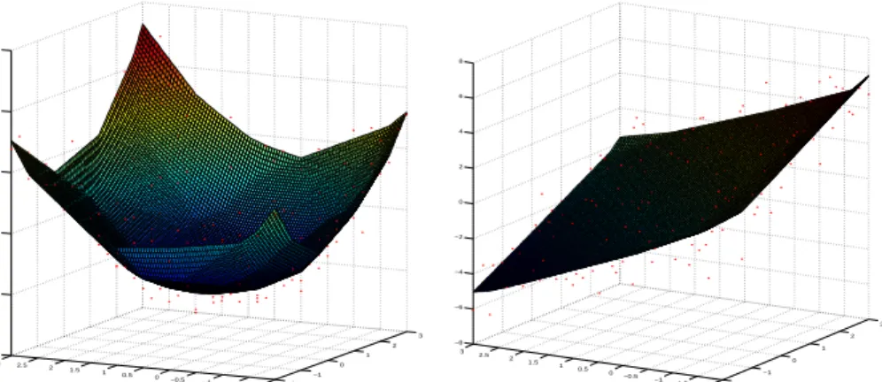
MOSEK and QPOPT. Here we present two simulated examples to illustrate the computation of the estimator when d = 2. The first one, depicted in Figure 2.1a corresponds to the case where φ(x) = |x|2. Figure 2.1b shows
the convex function estimator when the regression function is the hyperplane φ(x) = −x1 +x2. In both cases, n = 256 observations were used and the
errors were assumed to be i.i.d. from the standard normal distribution. All the computations were carried out using the MOSEK optimization toolbox
−2 −1 0 1 2 3 −2 −1.5 −1 −0.5 0 0.5 1 1.5 2 2.5 3 −5 0 5 10 15 20 −2 −1 0 1 2 3 −2 −1.5 −1 −0.5 0 0.5 1 1.5 2 2.5 3 −8 −6 −4 −2 0 2 4 6 8
Figure 2.1: The scatter plot and nonparametric least squares estimator of the convex regression function when (a) φ(x) = |x|2 (left panel); (b) φ(x) = −x1+x2 (right panel).
for Matlab and the run time for each example was less than 2 minutes in a standard desktop PC. We refer the reader to Kuosmanen (2008) for addi-tional numerical examples (although the examples there are for the estimation of concave, componentwise nondecreasing functions, the computational com-plexities are the same).
2.3
Consistency of the least squares estimator
The main goal of this paper is to show that in an appropriate setting the nonparametric least squares estimator ˆφn described above is consistent for
estimating the convex function φ on the set X. In this context, we will prove the consistency of ˆφn in both, fixed and stochastic design regression settings.
Before proceeding any further we would like to introduce some nota-tion. For any Borel set X⊂ Rd we will denote by B
X the σ-algebra of Borel subsets ofX. Given a sequence of events (An)∞n=1we will be using the notation
[An i.o.] and [An a.a.] to denote limAn and limAn, respectively.
Now, consider a convex function f : Rd →
R. This function is said to be proper if f(x) > −∞ for every x ∈ Rd. The effective domain of f,
denoted by dom(f), is the set of points x ∈ Rd for which f(x) < ∞. The
subdifferential of f at a point x ∈ Rd is the set ∂f(x) ⊂
Rd of all vectors ξ satisfying the inequality
hξ, hi ≤f(x+h)−f(x) ∀ h∈Rd.
The elements of ∂f(x) are called subgradients of f at x (see Rockafellar
(1970)). For a setA⊂Rdwe denote byA◦,Aand∂Aits interior, closure and
boundary, respectively. We write Ext(A) =Rd\A for the exterior of the set
Aand diam(A) := supx,y∈A|x−y|for the diameter ofA. We also use the sup-norm notation, i.e., for a function g :Rd→
Rwe write kgkA= supx∈A|g(x)|.
To avoid measurability issues regarding some sets, specially those in-volving the random set-valued functions{∂φˆn(x)}x∈X◦, we will use the symbols
P∗ and P∗ to denote inner and outer probabilities, respectively. We refer the
reader to van der Vaart and Wellner (1996), pages 6-15, for the basic prop-erties of inner and outer probabilities. In this context, a sequence of (not necessarily measurable) functions (Ψn)∞n=1 from a probability space (Ω,F,P)
into R is said to converge to a function Ψ almost surely (see van der Vaart and Wellner (1996), Definition 1.9.1-(iv), page 52), written Ψn
a.s.
−→ Ψ, if
P∗(Ψn →Ψ) = 1. We will use the standard notationP(A) for the
probabil-ities of all eventsA whose measurability can be easily inferred from the mea-surability of the random variables {φˆn(x)}x∈X, established in Lemma 2.2.4.
Our main theorems hold for both, fixed and stochastic design schemes, and the proofs are very similar. They differ only in minor steps. Therefore, for the sake of simplicity, we will denote the observed values of the regressor variables always with the capital letters Xn. For any Borel set X ⊂ Rd, we
write
Nn(X) = #{1≤j ≤n :Xj ∈X}.
The quantities Xn and Nn(X) are non-random under the fixed design but
random under the stochastic one.
2.3.1
Fixed Design
In a “fixed design” regression setting we assume that the regressor values are non-random and that all the uncertainty in the model comes from the response variable. We will now list a set of assumptions for this type of design. The one-dimensional case has been proven, under different regularity conditions, inHanson and Pledger (1976).
(A1) We assume that we have a sequence (Xn, Yn)
∞
n=1 satisfying
Yk =φ(Xk) +k
where (n)∞n=1 is an i.i.d. sequence with E(j) = 0, E 2j
= σ2 < ∞
and φ:Rd→
R is a proper convex function.
(A2) The non-random sequence (Xn)∞n=1 is contained in a closed, convex set
X⊂Rd with X◦ 6=∅ and X⊂dom(φ).
(A3) We assume the existence of a Borel measureν onX satisfying: (i) {X ∈ BX :ν(X) = 0}={X∈ BX:X has Lebesgue measure 0}. (ii) n1Nn(X)→ν(X) for any open rectangle X⊂X◦.
(A4) We assume that we have a sequence (Xn, Yn)
∞
n=1 satisfying
Yk =φ(Xk) +k
where φ : Rd → R is a proper convex function and (n)∞n=1 is an
inde-pendent sequence of random variables satisfying (i) E(n) = 0 ∀ n∈N and limn1
Pn k=1E(|k|)>0. (ii) P∞n=1 Var( 2 n) n2 <∞. (iii) supn∈N{E(2n)}<∞.
Under these conditions we define σ2 := limn→∞ n1Pnj=1E 2j
.
The raison d’etre of condition (A4) is to allow the variance of the error terms to depend on the regressors. We make the distinction between (A1) and (A4) because in the case of i.i.d. errors it is enough to require a finite second moment to ensure consistency.
2.3.2
Stochastic Design
In this setting we assume that (Xn, Yn)∞n=1 is an i.i.d. sequence from some
Borel probability measureµonRd+1. Here we make the following assumptions
on the measure µ:
(A5) There is a closed, convex setX⊂RdwithX◦ 6=∅such thatµ(X× R) = 1. Also,
Z
X×R
y2µ(dx, dy)<∞.
(A6) There is a proper convex function φ : Rd →
R with X ⊂ dom(φ) such that whenever (X, Y) ∼ µ we have E(Y −φ(X)|X) = 0 and
(A7) Denoting by ν(·) =µ((·)×R) the x-marginal of µ, we assume that
{X∈ BX:ν(X) = 0}={X ∈ BX :X has Lebesgue measure 0}. We wish to point out some conclusions that one can draw from these assumptions. Consider the class of functions
Kν := ψ :Rd→R | ψ is convex with Z |ψ(x)|2ν(dx)<∞ .
Then for any X⊂X the following holds
Z
X×R
ψ(x)(y−φ(x))µ(dx, dy) = 0 ∀ψ ∈ Kµ;
so we get that φ is in fact the element of Kµ which is the closest to Y in the
Hilbert space L2(X×R,BX×R, µ). This follows from Moreau’s decomposition
theorem (see the proof of Lemma 2.2.4).
Additionally, conditions {A5-A7} allow for stochastic dependency be-tween the error variable Y −φ(X) and the regressorX. Although some level of dependency can be put to satisfy conditions {A2-A4}, the measure µ al-lows us to take into account some cases which wouldn’t fit in the fixed design setting (even by conditioning on the regressors).
2.3.3
Main results
We can now state the two main results of this paper. The first result shows that assuming only the convexity ofφ, the least squares estimator can be used to consistently estimate both φ and its subdifferentials ∂φ(x).
Theorem 2.3.1 Under any of {A1-A3}, {A2-A4} or {A5-A7} we have,
(i) P
sup
x∈X
{|φˆn(x)−φ(x)|} →0 for any compact set X⊂X◦
(ii) For every x∈X◦ and every ξ∈Rd lim n→∞limh↓0 ˆ φn(x+hξ)−φˆn(x) h ≤limh↓0 φ(x+hξ)−φ(x) h almost surely.
(iii) Denoting by B the unit ball (w.r.t. the Euclidian norm) we have
P∗
∂φˆn(x)⊂∂φ(x) +B a.a.
= 1 ∀ >0, ∀ x∈X◦. (iv) If φ is differentiable at x∈X◦, then
sup
ξ∈∂φˆn(x)
{|ξ− ∇φ(x)|}−→a.s. 0.
Our second result states that assuming differentiability of φ on the entire X◦
allows us to use the subdifferentials of the least squares estimator to consis-tently estimate ∇φ uniformly on compact subsets of X◦.
Theorem 2.3.2 If φ is differentiable on X◦, then under any of {A1-A3},
{A2-A4} or {A5-A7} we have,
P∗ sup ξ∈∂φˆn(x) x∈X
{|ξ− ∇φ(x)|} →0 for any compact set X⊂X◦
= 1.
2.3.4
Proof of the main results
Before embarking on the proofs, one must notice that there are some state-ments which hold true under any of {A1-A3},{A2-A4} or{A5-A7}. We list the most important ones below, since they’ll be used later.
• For any set X⊂X we have Nn(X)
n
a.s.
• The strong law of large numbers implies that for any Borel set X ⊂ X
with positive Lebesgue measure we have 1 Nn(X) X Xk∈X 1≤k≤n (Yk−φ(Xk)) a.s. −→0 (2.10) and also lim n→∞ 1 n X 1≤k≤n (Yk−φ(Xk))2 =σ2 a.s. (2.11)
We would like to point out that in the case of condition A4, A4-(iii) allows us to obtain (2.10) from an application of a version of the strong law of large number for uncorrelated random variables, as it appears in Chung (2001), page 108, Theorem 5.1.2. Similarly, condition A4-(ii) implies that we can apply a version the strong law of large numbers for independent random variables as in Williams (1991), Lemma 12.8, page 118 or inFolland(1999), Theorem 10.12, page 322 to obtain (2.11).
• For any Borel subset X⊂X with positive Lebesgue measure, #{n ∈N:Xn ∈X}
a.s.
−→+∞ (2.12)
Proof of Theorem 2.3.1. We will only make distinctions among the design schemes in the proof if we are using any property besides (2.9), (2.10), (2.11) or (2.12). For the sake of clarity, we divide the proof in steps.
Step I:We start by showing that for any set with positive Lebesgue measure there is a uniform band around the regression function (over that set) such that ˆφn comes within the band at least at one point for all but finitely many
Lemma 2.3.1 For any set X ⊂X with positive Lebesgue measure we have, Pinf x∈X n |φˆn(x)−φ(x)| o ≥M i.o.= 0 ∀ M > pσ ν(X).
Step II: The idea is now to use the convexity of both, φ and ˆφn, to show
that the previous result in fact implies that the sup-norm of ˆφn is uniformly
bounded on compact subsets of X◦. We achieve this goal in the following two lemmas (whose proofs are given in Sections 2.4.2 and 2.4.3 respectively).
Lemma 2.3.2 LetX ⊂X◦ be compact with positive Lebesgue measure. Then, there is a positive real number KX such that
Pinf x∈X{ ˆ φn(x)}<−KX i.o. = 0.
Lemma 2.3.3 Let X ⊂ X◦ be a compact set with positive Lebesgue measure. Then, there is KX >0 such that
P sup x∈X {φˆn(x)} ≥KX i.o. = 0.
Step III:Convex functions are determined by their subdifferential mappings (seeRockafellar(1970), Theorem 24.9, page 239). Moreover, having a uniform upper boundKX for the norms of all the subgradients over a compact region X imposes a Lipschitz continuity condition on the convex function over X(see
Rockafellar (1970), Theorem 24.7, page 237); the Lipschitz constant being KX. For these reasons, it is important to have a uniform upper bound on the norms of the subgradients of ˆφn on compact regions. The following lemma
(proved in Section 2.4.4) states that this can be achieved.
Lemma 2.3.4 Let X ⊂ X◦ be a compact set with positive Lebesgue measure. Then, there is KX >0 such that
P∗ sup ξ∈∂φˆn(x) x∈X {|ξ|}> KX i.o. = 0.
Step IV: For the next results we need to introduce some further notation. We will denote by µn the empirical measure defined on Rd+1 by the sample
(X1, Y1), . . . ,(Xn, Yn). In agreement with van der Vaart and Wellner (1996),
given a class of functions G on D ⊂ Rd+1, a seminorm k·k on some space
containing G and >0 we denote by N(,G,k · k) the covering number of
G with respect tok · k.
Although Lemmas 2.3.5 and 2.3.7 may seem unrelated to what has been done so far, they are crucial for the further developments. Lemma 3.5 (proved in Section 2.4.5) shows that the class of convex functions is not very complex in terms of entropy. Lemma2.3.7 is a uniform version of the strong law of large numbers which proves vital in the proof of Lemma 2.3.8.
Lemma 2.3.5 Let X ⊂ X◦ be a compact rectangle with positive Lebesgue measure. For K > 0 consider the class GK,X of all functions of the form ψ(X)(Y −φ(X))1X(X) where ψ ranges over the class DK,X of all proper con-vex functions which satisfy
(a) kψkX ≤K;
(b) [
ξ∈∂ψ(x) x∈X
{ξ} ⊂[−K, K]d.
Then, for any >0 we have lim
n→∞N(,GK,X,L1(X×R, µn))<∞ almost surely,
and there is a positive constant A <∞, depending only on (X1, . . . , Xn), K
and X, such that the covering numbers N(n Pn
j=1|Yj −φ(Xj)|,GK,X,L1(X ×
R, µn)) are bounded above by A, for all n∈N, almost surely.
The proofs of Lemmas 2.3.7 and 2.3.8 (given in Sections 2.4.7 and 2.4.8 re-spectively) are the only parts in the whole proof where we must treat the
different design schemes separately. To make the argument work, a small lemma (proved in Section2.4.6) for the set of conditions{A2-A4}is required. We include it here for the sake of completeness and to point out the difference between the schemes.
Lemma 2.3.6 Consider the set of conditions {A2-A4} and a subsequence (nk)∞k=1 such that lim k→∞ 1 nk nk X j=1 E 2j =σ2.
Let (Xm)∞m=1 be a an increasing sequence of compact subsets of X satisfying
ν(Xm)→1. Then, lim m→∞klim→∞ 1 nk X {1≤j≤nk:Xj∈Xm} E 2j =σ2.
We are now ready to state the key result on the uniform law of large numbers.
Lemma 2.3.7 Consider the notation of Lemma 2.3.5 and let X ⊂X◦ be any finite union of compact rectangles with positive Lebesgue measure. Then,
sup ψ∈DK,X 1 n X {1≤j≤n:Xj∈X} ψ(Xj)(Yj−φ(Xj)) a.s. −→0.
Step V: With the aid of all the results proved up to this point, it is now possible to show that Lemma 2.3.1 is in fact true if we replace M by an arbitrarily smallη > 0. The proof of the following lemma is given in Section 2.4.8.
Lemma 2.3.8 LetX ⊂X◦ be any compact set with positive Lebesgue measure. Then, (i) Pinf x∈X{φ(x)− ˆ φn(x)} ≥η i.o. = 0 ∀ η >0,
(ii) P sup x∈X {φ(x)−φˆn(x)} ≤ −η i.o. = 0 ∀ η >0.
Step VI: Combining the last lemma with the fact that we have a uniform bound on the norms of the subgradients on compacts, we can state and prove the consistency result on compacts. This is done in the next lemma (proof included in Section 2.4.9).
Lemma 2.3.9 Let X ⊂ X◦ be a compact set with positive Lebesgue measure. Then, (i) Pinf x∈X{ ˆ φn(x)−φ(x)}<−η i.o. = 0 ∀ η >0, (ii) P sup x∈X {φˆn(x)−φ(x)}> η i.o. = 0 ∀ η >0, (iii) sup x∈X {|φˆn(x)−φ(x)|} a.s. −→0.
Step VII: We can now complete the proof of Theorem 2.3.1. Consider the class C of all open rectangles R such that R ⊂ X◦ and whose vertices have rational coordinates. Then, C is countable and S
R∈CR =X
◦. Observe that
Lemmas 2.3.2 and 2.3.3 imply that for any finite union A :=R1 ∪ · · · ∪ Rm
of open rectangles R1, . . . ,Rm ∈ C there is, with probability one, n0 ∈ N such that the sequence ( ˆφn)∞n=n0 is finite on Conv(A). From Lemma 2.3.9
we know that the least squares estimator converges at all rational points in
X◦ with probability one. Then, Theorem 10.8, page 90 of Rockafellar (1970) implies that (i) holds if X◦ is replaced by the convex hull of a finite union of rectangles belonging to C. Since there are countably many of such unions and any compact subset of X◦ is contained in one of those unions, we see that (i) holds. An application of Theorem 24.5, page 233 of Rockafellar (1970) on an open rectangle C containingx and satisfying C ⊂X◦ gives (ii) and (iii).
Proof of Theorem2.3.2. To prove the desired result we need the follow-ing lemma (whose proof is provided in Section 2.4.10) from convex analysis. The result is an extension of Theorem 25.7, page 248 of Rockafellar (1970), and might be of independent interest.
Lemma 2.3.10 Let C ⊂Rd be an open, convex set and f a convex function
which is finite and differentiable on C. Consider a sequence of convex func-tions (fn)∞n=1 which are finite on C and such that fn → f pointwise on C.
Then, if X ⊂ C is any compact set, sup
x∈X
ξ∈∂fn(x)
{|ξ− ∇f(x)|} →0.
Defining the classC of open rectangles as in the proof of Theorem 2.3.1, one can use a similar argument to obtain Theorem 2.3.2 from an application of
Theorem 2.3.1 and the previous lemma.
2.4
Proofs of auxiliary lemmas
Here we prove the lemmas involved in the proof of the main theorem. To prove these, we will need additional auxiliary results from matrix algebra and convex analysis, which may be of independent interest and are proved in the Appendix.
2.4.1
Proof of Lemma
2.3.1
We will first show that the eventh infx∈X n ˆ φn(x)−φ(x) o
≥M i.o.i has probability zero. Under this event, there is a subsequence (nk)∞k=1such that infx∈X
n
ˆ
φnk(x)−φ(x)
o
Then (2.10) implies that for this subsequence, with probability one, we have lim k→∞ 1 Nnk(X) X Xj∈X {Yj −φˆnk(Xj)} ≤ −M. (2.13)
On the other hand, it is seen (by solving the corresponding quadratic pro-gramming problems; see, e.g., Exercise 16.2, page 484 of Nocedal and Wright
(1999)) that for anyη >0, m∈N
inf ( 1 m X 1≤j≤m |ξj|2 : 1 m X 1≤j≤m ξj ≥η, ξ∈Rm ) = η2, (2.14) inf ( 1 m X 1≤j≤m |ξj|2 : 1 m X 1≤j≤m ξj ≤ −η, ξ∈Rm ) = η2. (2.15) For 0< δ < M, using (2.15) with η=M −δ together with (2.12) and (2.13) we get that, with probability one, we must have
lim k→∞ 1 nk nk X j=1 (Yj−φˆnk(Xj)) 2 ≥ν(X)(M −δ)2.
Letting δ→0 we actually get lim k→∞ 1 nk nk X j=1 (Yj−φˆnk(Xj)) 2 ≥ν(X)M2 > σ2 = lim k→∞ 1 nk nk X j=1 (Yj−φ(Xj))2 a.s.
which is impossible because ˆφnk is the least squares estimator. Therefore,
Pinf x∈X n ˆ φn(x)−φ(x) o ≥M i.o.= 0. A similar argument now using (2.14) gives
P sup x∈X n ˆ φn(x)−φ(x) o ≤ −M i.o. = 0,
which completes the proof of the lemma.
Before we prove Lemmas 2.3.2 and 2.3.3, we need some additional re-sults from matrix algebra. For convenience, we state them here, but postpone their proofs to Section B in the Appendix.
We first introduce some notation. We write ej ∈ Rd for the vector whose components are given by ek
j = δjk, where δjk is the Kronecker δ. We
also write e=e1+. . .+ed for the vector of ones in Rd. For α∈ {−1,1}d we write Rα = ( d X k=1 θkαkek :θ ≥0, θ ∈Rd )
for the orthant in theαdirection. For any hyperplaneHdefined by the normal vector ξ ∈ Rd and the intercept b ∈
R, we write H ={x ∈ Rd : hξ, xi =b},
H+ = {x ∈
Rd : hξ, xi > b} and H− = {x ∈ Rd : hξ, xi < b}. For r > 0 and x0 ∈Rd we will writeB(x0, r) ={x∈Rd :|x−x0|< r}. We denote by
Rd×d the space of d×d matrices endowed with the topology defined by the
k · k2 norm (where kAk2 = sup|x|≤1{|Ax|} and can be shown to be equal to
the largest singular value of A; see Harville (2008)).
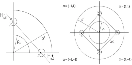
Lemma 2.4.1 Let r > 0. There is a constant Rr > 0, depending only on r
and d, such that for any ρ∗ ∈ (0, Rr) there are ρ, ρ∗ > 0 with the property:
for any α ∈ {−1,1}d and any d-tuple of vectors β ={x
1, . . . , xd} ⊂Rd such
that xj ∈ B(αjrej, ρ) ∀ j = 1, . . . , d, there is a unique pair (ξα,β, bα,β), with
ξα,β ∈Rd, |ξα,β|= 1 and bα,β >0 for which the following statements hold:
(i) β form a basis for Rd.
(ii) x1, . . . , xd ∈ Hα,β :={x∈Rd:hξα,β, xi=bα,β}. (iii) min 1≤j≤d{|ξ j α,β|}>0. (iv) B(0, ρ∗)⊂ H−α,β. (v) {x∈Rd:|x| ≥ρ∗} ∩ R α ⊂ H+α,β. (vi) B(−αjre j, ρ)⊂ {x∈Rd:hξα,β, xi<0} for all j = 1, . . . , d.
x1
x-1
x2
x-2
Figure 2.2: Explanatory diagram for (a) Lemma2.4.1(left panel); (b) Lemma 2.4.2 (right panel).
(vii) For any w1 ∈B
0, ρ∗ 16√d and w2 ∈B 3ρ∗ 8√dα, ρ∗ 8√d we have min 1≤j≤d n Xβ−1(w1+t(w2−w1)) jo >0 ∀ t≥1
where Xβ = (x1, . . . , xd)∈Rd×d is the matrix whose j’th column is xj.
Figure 2.2a illustrates the above lemma when d = 2 and α = (1,1). The lemma states that whatever points x1 and x2 are taken inside the circles
of radius ρ around α1re1 and α2re2, respectively, B(0, ρ∗) and {x ∈ Rd :
|x| ≥ρ∗} ∩ Rα are contained, respectively, in the half-spaces H−α,β and H + α,β.
Assertion (vii) of the lemma implies that all the points in the half line {w1+
t(w2−w1}t≥1 should have positive co-ordinates with respect to the basisβ as
they do with respect to the basis {αjej}dj=1. We refer the reader to Section
B.1 for a complete proof of Lemma 2.4.1.
We now state two other useful results, namely Lemma2.4.2and Lemma 2.4.3, but defer their proofs to Section B.2 and Section B.3 respectively.
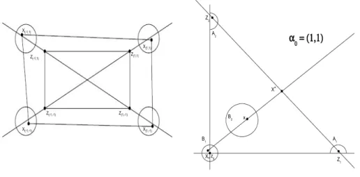
Lemma 2.4.2 Let r >0 and consider the notation of Lemma 2.4.1 with the positive numbersρ,ρ∗ andρ∗ as defined there. Take 2d vectors{x±1, . . . , x±d}
⊂Rdsuch that x
±j ∈B(±rej, ρ)and forα∈ {−1,1}d write βα ={xα11, xα22,
. . . , xαdd}, ξα = ξα,βα, bα = bα,βα and Hα = Hα,β, all in agreement with the setting of Lemma 2.4.1. Then, if K =Conv(x±1, . . . , x±d) we have:
(i) K =T α∈{−1,1}d{x∈Rd :hξα, xi ≤bα}. (ii) K◦ =T α∈{−1,1}d{x∈Rd :hξα, xi< bα}. (iii) ∂K =S α∈{−1,1}dConv(xα11, . . . , xαdd). (iv) ∂K= S α∈{−1,1}d{x∈Rd:hξα, xi=bα} TT α∈{−1,1}d{x∈Rd:hξα, xi ≤bα} . (v) B(0, ρ∗)⊂K◦. (vi) ∂B(0, ρ∗)⊂Ext(K).
Figure2.2b illustrates Lemma2.4.2 for the two-dimensional case. Intuitively, the idea is that as long as the points x±1 and x±2 belong to B(±re1, ρ) and
B(±re2, ρ), respectively, we will haveB(0, ρ∗) and ∂B(0, ρ∗) as subsets ofK◦
and Ext(K), respectively.
Z(1,1) Z(-1,-1) Z(1,-1) Z(-1,1) X(1,1) X(1,-1) X(-1,-1) X(-1,1) α0 = (1,1) z0 x X* B2 B1 X* A1 Z1 A2 Z2
Figure 2.3: Explanatory diagram for (a) Lemma2.4.3(left panel); (b) Lemma 2.3.2 (right panel).
Lemma 2.4.3 Let[a, b]⊂Rd be a compact rectangle andr > 0, withr < 1 d−2
if d≥3. For each α ∈ {−1,1}d write z
α =a+ Pd j=1 1+αj 2 (b j −aj)e j so that
{zα}α∈{−1,1}d is the set of vertices of [a, b]. Then, there is ρ > 0 such that if xα ∈B(zα+r(zα−z−α), ρ) ∀ α∈ {−1,1}d, then
[a, b]⊂Conv xα :α∈ {−1,1}d
◦
.
Figure2.3a describes Lemma2.4.3in the two-dimensional case. As long as the pointsx(±1,±1) are chosen in the balls of radiusρaroundz(±1,±1)+r(z(±1,±1)−
z(∓1,∓1)),Conv x(±1,±1)
will contain Conv z(±1,±1)
.
2.4.2
Proof of Lemma
2.3.2
Since any compact subset of X◦ is contained in a finite union of compact rectangles, it is enough to prove the result when X is a compact rectangle [a, b] ⊂ X◦. Let r = 14min1≤k≤d{bk−ak} and choose ρ ∈ (0,14r), ρ∗ >0 and
0< ρ∗ < 12r such that the conclusions of Lemmas2.4.1and 2.4.2hold for any
α ∈ {−1,1}d and any β = (z 1, . . . , zd) ∈ Rd×d with zj ∈ B(αjrej, ρ). Take N ∈N such that 1 N 1max≤k≤d{b k−ak}< 1 32dρ∗ (2.16)
and divide X into Nd rectangles all of which are geometrically identical to
1
N[0, b−a]. Let C be any one of the rectangles in the grid and choose any
vertex z0 of C satisfying z0 = argmax z∈C max 1≤j≤d zj −aj, bj−zj .
Then, from the definition ofz0 and r, there is α0 ∈ {−1,1}d such that
Additionally, define B1 = B z0, ρ∗ 16√d , B2 = B z0+ 3ρ∗ 8√dα0, ρ∗ 8√d , Aj = B(z0+αj0rej, ρ)∩(z0+Rα0) ∀j = 1, . . . , d, A−j = B(z0−α0jrej, ρ) ∀ j = 1, . . . , d.
Observe that all the sets in the previous display have positive Lebesgue mea-sure and that the A−j’s are not necessarily contained in X. Let M1 = kφkX,
M0 > √ σ
min{ν(B1),ν(B2),ν(A1),...,ν(Ad)}
,M =M1+M0 andKC >6M. Also, notice
that C ⊂B1 because of (2.16). We will argue that P inf x∈C{ ˆ φn(x)} ≤ −KC i.o. = 0. (2.17)
From Lemma 2.3.1, we know that
P d \ j=1 inf x∈Aj n ˆ φn(x)−φ(x) o < M0 a.a. ! = 1, (2.18)
so there is, with probability one,n0 ∈Nsuch that infx∈Aj
n ˆ φn(x)−φ(x) o < M0 for any n≥n0 and any j = 1, . . . , d.
Assume that the eventhinfx∈C{φˆn(x)}<−KC i.o. i
is true. Then, there is a subsequence nk such that infx∈C{φˆnk(x)} < −KC for all k ∈N. Fix any k ≥ n0. We know that there is X∗ ∈ C ⊂ B1 such that ˆφnk(X∗) ≤ −KC. In addition, for j = 1, . . . , d, there are Zαj
0j ∈ Aj such that |
ˆ
φnk(Zαj0j) −
φ(Zαj
0j)| < M0, which in turn implies ˆφnk(Zα
j
0j)< M. Pick any Z−α
j
0 ∈ A−j
and let K =Conv(Z±1, . . . , Z±d) =z0+Conv(Z±1−z0, . . . , Z±d−z0).
Take anyx∈B2. We will show the existence ofX∗ ∈Conv
Zα1
01, . . . , Zαd0d
such that x∈Conv(X∗, X∗), as shown in Figure2.3b for the cased= 2. We
will then show that the existence of such an X∗ implies that
Consequently, since x is an arbitrary element of B2 we will have inf x∈C{ ˆ φn(x)} ≤ −KC i.o. ∩ d \ j=1 inf x∈Aj n ˆ φn(x)−φ(x) o < M0 a.a. ! ⊂ inf x∈B2 {|φ(x)−φˆnk(x)|} ≥M0 i.o. .
But from Lemma 2.3.1, the event on the right is a null set. Taking (2.18) into account, we will see that (2.17) holds and then complete the argument by taking KX = maxC{KC}.
To show the existence of X∗ consider the function ψ : R → Rd given
byψ(t) =X∗+t(x−X∗). The function ψ is clearly continuous and satisfies
ψ(0) = X∗ and ψ(1) = x ∈ B2 ⊂ K◦. That B2 ⊂ K◦ is a consequence
of Lemma 2.4.1, (iv). The set K is bounded, so there is T > 1 such that ψ(T)∈Ext(K) = Rd\K. The intermediate value theorem then implies that there is t∗ ∈ (1, T) such that X∗ := ψ(t∗) ∈ ∂K. Observe that by Lemma 2.4.2 (iii) we have
∂K = [
α∈{−1,1}d
Conv(Zα11, . . . , Zαdd).
Lemma2.4.1(i) implies that{Zα1
01−z0, . . . , Zαd0d−z0}forms a basis ofR dso we can writeX∗−z0 = Pd j=1θ j(Z
αj0j−z0). Moreover, Lemma 2.4.1(vii) implies
that θj >0 for everyj = 1, . . . , d asθ = (θ1, . . . , θd) = (Zα1
01−z0, . . . , Zαd0d−
z0)−1(X∗ − z0). Here we apply Lemma 2.4.1 (vii) with w1 = X∗ ∈ B1,
w2 =x∈B2 and t∗ >1.
For α ∈ {−1,1}d consider the pair (ξ
α, bα) ∈ Rd ×R as defined in
Lemma2.4.2for the set of vectors{Z±1−z0, . . . , Z±d−z0}(here we move the
origin toz0). Observe that Lemma2.4.1(ii) implies thathξα0, Zαj0j−z0i=bα0
for all j = 1, . . . , d. Consequently, hξα0, X
∗ −z
0i = bα0
Pd
j=1θ
X∗ ∈ ∂K, Lemma 2.4.2 (iv) implies that hξα0, X
∗ −z
0i ≤ bα0 and hence
Pd
j=1θj ≤1. Additionally, for α6=α0 we can write hξα, X∗−z0ias d X j=1 θjhξα, Zαj 0j−z0i= X αj=αj 0 θjbα+ X αj6=αj 0 θjhξα, Zαj 0j −z0i< bα (2.20)
as hξα, Zαj −z0i = bα (by Lemma 2.4.1 (ii)) and hξα, Z−αj −z0i < 0 (by Lemma 2.4.1 (vi)) for every j = 1, . . . , d. Since hξα, w − z0i = bα for
all w ∈ Conv(Zα11, . . . , Zαdd) and all α ∈ {−1.1}d, (2.20) and the fact that X∗ ∈ ∂K imply that X∗ ∈ ConvZα1
01, . . . , Zαd0d . Hence ˆφn(X∗) ≤ Pd j=1θjφˆnk(Zαj0j)< M. We therefore have ˆ φnk(X ∗ )< M , φˆnk(X∗)<−KC, (2.21) X∗ + 1 t∗(X ∗− X∗) = x. (2.22)
Since X∗ ∈B1 and d≥1 we have |z0−X∗|<
1
8ρ∗. (2.23)
By using the triangle inequality we get the following bounds 1
4ρ∗ <|z0−x|< 1
2ρ∗. (2.24)
And from Lemma 2.4.1 (iv) and the fact thathξα0, X
∗i=b
α0 we also obtain
|z0−X∗| ≥ρ∗. (2.25)
From (2.22) we know that t∗ = |X∗−X∗|
|x−X∗| . Using the triangle inequality with
(2.23), (2.24) and (2.25) one can find lower and upper bounds for|X∗−X∗|(as
|X∗−X∗| ≥ |X∗−z0|−|z0−X∗|) and|x−X∗|(as|x−X∗| ≤ |x−z0|+|z0−X∗|),
respectively, to obtain t∗ ≥ 7
5. Then, (2.21) and (2.22) imply
ˆ φnk(x)≤ 1− 1 t∗ ˆ φnk(X∗) + 1 t∗φˆnk(X ∗ )≤ −2 7KC+ 5 7M <−M.
Consequently,
|φ(x)−φˆnk(x)|> M −M1 =M0.
This proves (2.19) and completes the proof.
2.4.3
Proof of Lemma
2.3.3
Assume without loss of generality thatXis a compact rectangle. Let{zα :α ∈
{−1,1}d}be the set of vertices of the rectangle. Then, there isr ∈(0,1) such
that B(zα, r) ⊂ X◦ ∀ α ∈ {−1,1}d. Recall that from Lemma 2.4.3, there is
0< ρ < 12rsuch that for any{ηα :α ∈ {−1,1}d}ifηα ∈B(zα+r2(zα−z−α), ρ)
then X⊂Conv ηα :α∈ {−1,1}d . Let Aα =B(zα+12r(zα−z−α),ρ2) and M0 > √ σ min{ν(Aα):α∈{−1,1}d} and choose M1 = sup x∈Conv(S α∈{−1,1}dAα) {|φ(x)|}. TakeKX > M0+M1. Since P \ α∈{−1,1}d inf x∈Aα {|φˆn(x)−φ(x)|}< M0, a.a. = 1
by Lemma 2.3.1, there is, with probability one, n0 ∈ N such that for any
n ≥n0 we can find ηα ∈Aα, α∈ {−1,1}d, such that |φˆn(ηα)−φ(ηα)|< M0.
It follows that ˆφn(ηα)≤KX ∀α ∈ {−1,1}d. Now, using Lemma2.4.3we have X⊂Conv ηα :α∈ {−1,1}d
and the convexity of ˆφnimplies that ˆφn(x)≤KX
for any x∈X.
2.4.4
Proof of Lemma
2.3.4
Assume that X = [a, b] is a rectangle with vertices {zα : α ∈ {−1,1}d}.
x∗ ∈ ∂X such that ψ(x∗) = infx∈∂X{ψ(x)}. Observe that ψ(x∗) > 0 because
x∗ ∈ ∂X⊂ X◦. By Lemma2.4.3, there is a r < 12ψ(x∗) for which there exists
ρ < 1
4r such that whenever ηα ∈ Aα := B
zα+34r zα−z−α |zα−z−α| , ρ for any α∈ {−1,1}d and Kz = Conv zα+ 1 2r zα−z−α |zα−z−α| :α∈ {−1,1}d Kη = Conv ηα :α ∈ {−1,1}d we have X⊂Kz ⊂Kη◦ ⊂Kη ⊂X◦. (2.26) LetM0 > √ σ min{ν(Aα):α∈{−1,1}d}
and M1 ∈R be such that
Pinf x∈X{ ˆ φn(x)} ≤ −M0 i.o. = 0 and M1 = sup x∈Conv(S α∈{−1,1}dAα) {φ(x)}.
From Lemmas2.3.1 and 2.3.2 we can find, with probability one, n0 ∈N such
that infx∈X{φˆn(x)}>−M0 and infx∈Aα{|φˆn(x)−φ(x)|}< M0 for any n≥n0. Define M = M1 +M0 KX = 4|b−a| rmin1≤j≤d{bj−aj} M
and take any n ≥n0. Then, for any α ∈ {−1,1}d we can find ηα ∈ Aα such
that |φˆn(ηα)−φ(ηα)| < M0. Then, (2.26) implies that ˆφn(x) ≤ M ∀x ∈ X.
Take then x ∈ X and ξ ∈ ∂φˆn(x). A connectedness argument, like the one
used in the proof of Lemma 2.3.2, implies that there is t∗ > 0 such that
x+t∗ξ ∈∂Kη. But then we must have t∗ >
rmin1≤j≤d{bj−aj}
2|ξ||b−a| as a consequence
of (2.26), since the