10-705/36-705 Intermediate Statistics
Larry Wasserman
http://www.stat.cmu.edu/~larry/=stat705/
Fall 2011
Week
Class I
Class II
Day III
Class IV
Syllabus
August 29 Review Review, Inequalities Inequalities
September 5 No Class O P HW 1 [soln] VC Theory
September 12 Convergence Convergence HW 2 [soln] Test I
September 19 Convergence Addendum Sufficiency HW 3 [soln] Sufficiency
September 26 Likelihood Point Estimation HW 4 [soln] Minimax Theory
10-705/36-705: Intermediate Statistics, Fall 2010
Professor Larry Wasserman Office Baker Hall 228 A Email [email protected]
Phone 268-8727
Office hours Mondays, 1:30-2:30 Class Time Mon-Wed-Fri 12:30 - 1:20 Location GHC 4307
TAs Wanjie Wang and Xiaolin Yang
Website http://www.stat.cmu.edu/∼larry/=stat705
Objective
This course will cover the fundamentals of theoretical statistics. Topics include: point and in-terval estimation, hypothesis testing, data reduction, convergence concepts, Bayesian inference, nonparametric statistics and bootstrap resampling. We will cover Chapters 5 – 10 from Casella and Berger plus some supplementary material. This course is excellent preparation for advanced work in Statistics and Machine Learning.
Textbook
Casella, G. and Berger, R. L. (2002).Statistical Inference, 2nd ed.
Background
I assume that you are familiar with the material in Chapters 1 - 4 of Casella and Berger.
Other Recommended Texts
Wasserman, L. (2004). All of Statistics: A concise course in statistical inference. Bickel, P. J. and Doksum, K. A. (1977).Mathematical Statistics.
Rice, J. A. (1977).Mathematical Statistics and Data Analysis, Second Edition.
Grading
10% : Test I (Sept. 16) on the material of Chapters 1–4 20% : Test II (October 14)
20% : Test III (November 7)
30% : Final Exam (Date set by the University) 20% : Homework
Exams
All exams are closed book.Do NOT buy a plane ticket until the final exam has been scheduled. Homework
Homework assigments will be posted on the web. Hand in homework to Mari Alice Mcshane, 228 Baker Hall by3 pm Thursday. No late homework.
Reading and Class Notes
Class notes will be posted on the web regularly. Bring a copy to class.The notes are not meant to be a substitute for the book and hence are generally quite terse. Read both the notes and the text before lecture. Sometimes I will cover topics from other sources.
Group Work
You are encouraged to work with others on the homework. But write-up your final solutions on your own.
Course Outline
1. Quick Review of Chapters 1-4 2. Inequalities 3. Vapnik-Chervonenkis Theory 4. Convergence 5. Sufficiency 6. Likelihood 7. Point Estimation 8. Minimax Theory 9. Asymptotics 10. Robustness 11. Hypothesis Testing 12. Confidence Intervals 13. Nonparametric Inference 14. Prediction and Classification 15. The Bootstrap
16. Bayesian Inference
Lecture Notes 1
Quick Review of Basic Probability
(Casella and Berger Chapters 1-4)
1
Probability Review
Chapters 1-4 are a review. I will assume you have read and understood Chapters 1-4. Let us recall some of the key ideas.
1.1
Random Variables
A random variable is a map X from a probability space Ω to R. We write
P(X ∈A) = P({ω ∈Ω : X(ω)∈A})
and we write X ∼ P to mean that X has distribution P. The cumulative distribution function (cdf ) of X is
FX(x) = F(x) = P(X ≤x). IfX is discrete, its probability mass function (pmf )is
pX(x) =p(x) =P(X =x).
IfX is continuous, then its probability density function function (pdf ) satisfies
P(X ∈A) = Z A pX(x)dx= Z A p(x)dx
and pX(x) =p(x) =F0(x). The following are all equivalent:
X ∼P, X ∼F, X ∼p.
Suppose that X ∼P and Y ∼Q. We say that X and Y have the same distribution if
P(X ∈A) = Q(Y ∈A)
for all A. In other words, P = Q. In that case we say that X and Y are equal in distribution and we write X =d Y. It can be shown that X =d Y if and only if
FX(t) =FY(t) for all t.
1.2
Expected Values
The mean or expected value of g(X) is
E(g(X)) = Z g(x)dF(x) = Z g(x)dP(x) = ( R∞ −∞g(x)p(x)dx if X is continuous P jg(xj)p(xj) if X is discrete.
Recall that:
1. E(Pkj=1cjgj(X)) = Pkj=1cjE(gj(X)). 2. If X1, . . . , Xn are independent then
E n Y i=1 Xi ! =Y i E(Xi). 3. We often write µ=E(X).
4. σ2 =Var(X) = E((X−µ)2) is theVariance. 5. Var(X) =E(X2)−µ2.
6. If X1, . . . , Xn are independent then
Var n X i=1 aiXi ! =X i a2iVar(Xi). 7. The covariance is Cov(X, Y) = E((X−µx)(Y −µy)) =E(XY)−µXµY
and the correlation is ρ(X, Y) =Cov(X, Y)/σxσy. Recall that −1≤ρ(X, Y)≤1. The conditional expectation of Y given X is the random variableE(Y|X) whose value, when X =x is
E(Y|X =x) =
Z
y p(y|x)dy
where p(y|x) = p(x, y)/p(x). TheLaw of Total Expectation orLaw of Iterated Expectation:
E(Y) =EE(Y|X) =
Z
E(Y|X =x)pX(x)dx. The Law of Total Variance is
1.3
Exponential Families
A family of distributions{p(x;θ) : θ ∈Θ} is called an exponential family if
p(x;θ) = h(x)c(θ) exp ( k X i=1 wi(θ)ti(x) ) .
Example 1 X ∼Poisson(λ) is exponential family since
p(x) = P(X =x) = e −λλx x! = 1 x!e −λexp{logλ·x}.
Example 2 X ∼U(0, θ) is not an exponential family. The density is
pX(x) = 1
θI(0,θ)(x)
where IA(x) = 1 if x∈A and 0 otherwise.
We can rewrite an exponential family in terms of a natural parameterization. Fork = 1 we have p(x;η) =h(x) exp{ηt(x)−A(η)} where A(η) = log Z h(x) exp{ηt(x)}dx.
For example a Poisson can be written as
p(x;η) = exp{ηx−eη}/x! where the natural parameter is η= logλ.
Let X have an exponential family distribution. Then
E(t(X)) =A0(η), Var(t(X)) =A00(η).
Practice Problem: Prove the above result.
1.4
Transformations
LetY =g(X). Then FY(y) = P(Y ≤y) =P(g(X)≤y) = Z A(y) pX(x)dx where Ay ={x: g(x)≤y}. Then pY(y) =FY0(y). If g is monotonic, then pY(y) =pX(h(y)) dhdy(y)Example 3 Let pX(x) = e−x for x >0. Hence FX(x) = 1−e−x. Let Y = g(X) = logX. Then FY(y) = P(Y ≤y) = P(log(X)≤y) = P(X ≤ey) = FX(ey) = 1−e−e y and pY(y) =eye−e y for y∈R.
Example 4 Practice problem. Let X be uniform on (−1,2) and let Y =X2. Find the density of Y.
Let Z =g(X, Y). For exampe, Z =X+Y or Z =X/Y. Then we find the pdf of Z as follows:
1. For each z, find the setAz ={(x, y) :g(x, y)≤z}. 2. Find the CDF FZ(z) = P(Z ≤z) = P(g(X, Y)≤z) =P({(x, y) :g(x, y)≤z}) = Z Z Az pX,Y(x, y)dxdy. 3. The pdf is pZ(z) =FZ0(z).
Example 5 Practice problem. Let(X, Y) be uniform on the unit square. LetZ =X/Y. Find the density of Z.
1.5
Independence
Recall that X and Y are independent if and only if
P(X ∈A, Y ∈B) =P(X ∈A)P(Y ∈B) for all A and B.
Theorem 6 Let (X, Y) be a bivariate random vector with pX,Y(x, y). X and Y are inde-pendent iff pX,Y(x, y) = pX(x)pY(y).
1.6
Important Distributions
X ∼N(µ, σ2) if p(x) = 1 σ√2πe −(x−µ)2/(2σ2) . IfX ∈Rd then X ∼N(µ,Σ) if p(x) = 1 (2π)d/2|Σ|exp −1 2(x−µ) TΣ−1(x−µ) . X ∼χ2 p if X = Pp j=1Zj2 where Z1, . . . , Zp ∼N(0,1).X ∼Bernoulli(θ) if P(X = 1) =θ and P(X = 0) = 1−θ and hence
p(x) = θx(1−θ)1−x x= 0,1. X ∼Binomial(θ) if p(x) = P(X =x) = n x θx(1−θ)n−x x∈ {0, . . . , n}. X ∼Uniform(0, θ) if p(x) =I(0≤x≤θ)/θ.
1.7
Sample Mean and Variance
The sample mean isX = 1
n
X i
Xi,
and the sample variance is
S2 = 1
n−1
X i
(Xi−X)2.
LetX1, . . . , Xn be iid with µ=E(Xi) = µand σ2 =Var(Xi) = σ2. Then
E(X) = µ, Var(X) = σ 2 n, E(S 2) =σ2. Theorem 7 If X1, . . . , Xn ∼N(µ, σ2) then (a) X ∼N(µ, σn2) (b) (n−σ1)2S2 ∼χ2n−1
1.8
Delta Method
IfX ∼N(µ, σ2), Y =g(X) and σ2 is small then
Y ≈N(g(µ), σ2(g0(µ))2).
To see this, note that
Y =g(X) =g(µ) + (X−µ)g0(µ) + (X−µ) 2
2 g 00(ξ) for some ξ. Now E((X−µ)2) =σ2 which we are assuming is small and so
Y =g(X)≈g(µ) + (X−µ)g0(µ).
Thus
E(Y)≈g(µ), Var(Y)≈(g0(µ))2σ2.
Hence,
g(X)≈N g(µ), (g0(µ))2σ2.
Appendix: Useful Facts
Facts about sums
• Pni=1i= n(n+1) 2 . • Pni=1i2 = n(n+1)(2n+1) 6 . • Geometric series: a+ar+ar2+. . .= a 1−r, for 0 < r <1. • Partial Geometric seriesa+ar+ar2+. . .+arn−1 = a(1−rn)
1−r . • Binomial Theorem
n
Common Distributions
Discrete
Uniform • X ∼U(1, . . . , N) • X takes values x= 1,2, . . . , N • P(X =x) = 1/N • E(X) =PxxP(X =x) =Pxx1 N = 1 N N(N+1) 2 = (N+1) 2 • E(X2) =P xx2P(X =x) = P xx2 1N = 1 N N(N+1)(2N+1) 6 Binomial • X ∼Bin(n, p) • X takes values x= 0,1, . . . , n • P(X =x) = nxpx(1−p)n−x Hypergeometric • X ∼Hypergeometric(N, M, K) • P(X =x) = ( M x)( N−M K−x) (N K) Geometric • X ∼Geom(p) • P(X =x) = (1−p)x−1p,x= 1,2, . . . • E(X) =Pxx(1−p)x−1 =pP xdpd (−(1−p) x) =pp p2 = 1p. Poisson • X ∼Poisson(λ) • P(X =x) = e−xλ!λx x= 0,1,2, . . . • E(X) =Var(X) = λ P∞ tx e−λλx −λP∞ (λet) x −λ λet λ(et−1)• E(X) =λeteλ(et−1)
|t=0 =λ.
• Use mgf to show: if X1 ∼ Poisson(λ1), X2 ∼ Poisson(λ2), independent then Y =
X1+X2 ∼Poisson(λ1+λ2).
Continuous Distributions
Normal • X ∼N(µ, σ2) • p(x) = √1 2πσexp{ −1 2σ2(x−µ)2},x∈ R • mgfMX(t) = exp{µt+σ2t2/2}. • E(X) =µ • Var(X) =σ2.• e.g., IfZ ∼N(0,1) and X =µ+σZ, then X ∼N(µ, σ2). Show this...
Proof. MX(t) = E etX =E et(µ+σZ)=etµE etσZ = etµMZ(tσ) =etµe(tσ) 2/2 =etµ+t2σ2/2 which is the mgf of aN(µ, σ2). Alternative proof: FX(x) = P(X ≤x) = P(µ+σZ ≤x) = P Z ≤ x−µ σ = FZ x−µ σ pX(x) = FX0 (x) =pZ x−µ σ 1 σ
Gamma
• X ∼Γ(α, β).
• pX(x) = Γ(α1)βαxα−1e−x/β, x a positive real.
• Γ(α) =R0∞ 1
βαxα−1e−x/βdx.
• Important statistical distribution: χ2
p = Γ(p2,2). • χ2 p = Pp i=1Xi2, whereXi ∼N(0,1), iid. Exponential • X ∼exponen(β) • pX(x) = 1βe−x/β, x a positive real. • exponen(β) = Γ(1, β).
• e.g., Used to model waiting time of a Poisson Process. Suppose N is the number of phone calls in 1 hour and N ∼ P oisson(λ). Let T be the time between consecutive phone calls, then T ∼exponen(1/λ) and E(T) = (1/λ).
• IfX1, . . . , Xn are iid exponen(β), then PiXi ∼Γ(n, β). • Memoryless Property: If X ∼exponen(β), then
P(X > t+s|X > t) = P(X > s).
Linear Regression
Model the response (Y) as a linear function of the parameters and covariates (x) plus random error ().
Yi =θ(x, β) +i where
Generalized Linear Model
Model the natural parameters as linear functions of the the covariates.
Example: Logistic Regression.
P(Y = 1|X =x) = e
βTx
1 +eβTx.
In other words, Y|X =x∼Bin(n, p(x)) and
η(x) = βTx where η(x) = log p(x) 1−p(x) .
Logistic Regression consists of modelling the natural parameter, which is called the log odds ratio, as a linear function of covariates.
Location and Scale Families, CB 3.5
Letp(x) be a pdf. Location family : {p(x|µ) =p(x−µ) : µ∈R} Scale family : p(x|σ) = 1 σf x σ : σ >0Location−Scale family :
p(x|µ, σ) = 1 σf x−µ σ : µ∈R, σ >0
(1) Location family. Shifts the pdf.
e.g., Uniform with p(x) = 1 on (0,1) and p(x−θ) = 1 on (θ, θ+ 1).
Multinomial Distribution
The multivariate version of a Binomial is called a Multinomial. Consider drawing a ball from an urn with has balls with k different colors labeled “color 1, color 2, . . . , color k.”
Let p= (p1, p2, . . . , pk) where Pjpj = 1 and pj is the probability of drawing color j. Draw
n balls from the urn (independently and with replacement) and let X = (X1, X2, . . . , Xk) be the count of the number of balls of each color drawn. We say that X has a Multinomial (n, p) distribution. The pdf is p(x) = n x1, . . . , xk px1 1 . . . p xk k .
Multivariate Normal Distribution
We now define the multivariate normal distribution and derive its basic properties. We want to allow the possibility of multivariate normal distributions whose covariance matrix is not necessarily positive definite. Therefore, we cannot define the distribution by its density function. Instead we define the distribution by its moment generating function. (The reader may wonder how a random vector can have a moment generating function if it has no density function. However, the moment generating function can be defined using more general types of integration. In this book, we assume that such a definition is possible but find the moment generating function by elementary means.) We find the density function for the case of positive definite covariance matrix in Theorem 5.
Lemma 8 (a). Let X =AY+b Then
MX(t) = exp (b0t)MY(A0t). (b). Let c be a constant. Let Z =cY. Then
MZ(t) =MY(ct). (c). Let Y= Y1 Y2 , t= t1 t2 Then MY 1(t1) =MY t1 0 .
(d). Y1 and Y2 are independent if and only if
MY t1 t2 =MY t1 0 MY 0 t2 .
We start with Z1, . . . , Zn independent random variables such that Zi ∼ N1(0,1). Let Z = (Z1, . . . , Zn)0. Then E(Z) = 0, cov(Z) =I, MZ(t) =Yexpt 2 i 2 = exp t0t 2 . (1)
Letµ be an n×1 vector and A ann×n matrix. Let Y =AZ +µ. Then
E(Y) =µ cov(Y) = AA0. (2)
Let Σ = AA0. We now show that the distribution of Y depends only on µ and Σ. The moment generating functionMY(t) is given by
MY(t) = exp(µ0t)MZ(A0t) = exp µ0t+ t0(A 0A)t 2 = exp µ0t+ t0Σt 2 .
With this motivation in mind, letµbe ann×1 vector, and let Σ be a nonnegative definiten×n
matrix. Then we say that then-dimensional random vectorYhas an n-dimensional normal distribution with mean vector µ, and covariance matrix Σ, if Y has moment generating function MY(t) = exp µ0t+ t 0Σt 2 . (3)
We write Y ∼ Nn(µ,Σ). The following theorem summarizes some elementary facts about multivariate normal distributions.
Theorem 9 (a). If Y ∼Nn(µ,Σ), then E(Y) =µ, cov(Y) = Σ. (b). If Y ∼Nn(µ,Σ), c is a scalar, then cY∼Nn(cµ, c2Σ).
(c). Let Y ∼Nn(µ,Σ). If A is p×n, b is p×1, then AY+b∼Np(Aµ+b,AΣA0). (d). Let µbe any n×1 vector, and letΣ be any n×n nonnegative definite matrix. Then there exists Y such that Y∼Nn(µ,Σ).
Proof. (a). This follows directly from (2) above. (b) and (c). Homework.
(d). Let Z1, . . . , Zn be independent, Zi ∼ N(0,1). Let Z = (Z1, . . . , Zn)0. It is easily verified thatZ ∼Nn(0, I). LetY= Σ1/2Z+µ. By part b, above,
Theorem 10 Suppose that Y∼Nn(µ,Σ). Let Y= Y1 Y2 , µ= µ1 µ2 , Σ = Σ11Σ12 Σ21Σ22 .
where Y1 and µ1 are p×1, and Σ11 isp×p. (a). Y1 ∼Np(µ1,Σ11),Y2 ∼Nn−p(µ2,Σ22).
(b). Y1 and Y2 are independent if and only if Σ12= 0.
(c). If Σ22 >0, then the condition distribution of Y1 given Y2 is
Y1|Y2 ∼Np(µ1+ Σ12Σ−221(Y2−µ2),Σ11−Σ12Σ−221Σ21).
Proof. (a). Lett0 = (t01,t02) wheret1 is p×1. The joint moment generating function of
Y1 and Y2 is MY(t) = exp(µ01t1+µ02t2+ 1 2(t 0 1Σ11t1+t01Σ12t2+t02Σ21t1+t02Σ22t2)). Therefore, MY t1 0 = exp(µ01t1+ 1 2t 0 1Σ11t1), MY 0 t2 = exp(µ02t2+ 1 2t 0 2Σ22t2). By Lemma 1c, we see that Y1 ∼Np(µ1,Σ11),Y2 ∼Nn−p(µ2,Σ22).
(b). We note that MY(t) = MY t1 0 MY 0 t2 if and only if t01Σ12t2 +t02Σ21t1 = 0.
Since Σ is symmetric and t02Σ21t1 is a scalar, we see that t02Σ21t1 =t01Σ12t2. Finally, t0Σ
12t2 = 0 for all t1 ∈ Rp,t2 ∈ Rn−p if and only if Σ12 = 0, and the result follows from Lemma 1d.
(c). We first find the joint distribution of
X=Y1−Σ12Σ−221Y2 and Y2. X Y2 = I −Σ12Σ−122 0 I Y1 Y2
Therefore, by Theorem 2c, the joint distribution of X and Y2 is
X Y2 ∼Nn µ1−Σ12Σ−122µ2 µ2 , Σ11−Σ12Σ−122Σ21 0 0 Σ22
and henceX andY2 are independent. Therefore, the conditional distribution ofX givenY2 is the same as the marginal distribution of X,
SinceY2 is just a constant in the conditional distribution ofXgivenY2 we have, by Theorem 2c, that the conditional distribution of Y1 =X+ Σ12Σ−221Y2 given Y2 is
Y1|Y2 ∼Np(µ1−Σ12Σ−221µ2+ Σ12Σ−221Y2,Σ11−Σ12Σ−221Σ21) Note that we need Σ22>0 in part c so that Σ−122 exists.
Lemma 11 Let Y ∼Nn(µ, σ2I), where Y0 = (Y1, . . . , Yn), µ0 = (µ1, . . . , µn) and σ2 >0is a scalar. Then the Yi are independent, Yi ∼N1(µ, σ2) and
||Y||2 σ2 = Y0Y σ2 ∼χ 2 n µ0µ σ2 .
Proof. Let Yi be independent, Yi ∼ N1(µi, σ2). The joint moment generating function of the Yi is MY(t) = n Y i=1 (exp(µiti+ 1 2σ 2t2 i)) = exp(µ0t+ 1 2σ 2t0t)
which is the moment generating function of a random vector that is normally distributed with mean vector µ and covariance matrix σ2I. Finally, Y0Y = ΣY2
i , µ0µ = Σµ2i and
Yi/σ ∼N1(µi/σ,1). Therefore Y0Y/σ2 ∼χ2n(µ0µ/σ2) by the definition of the noncentral χ2 distribution.
We are now ready to derive the nonsingular normal density function.
Theorem 12 Let Y∼Nn(µ,Σ), with Σ>0. Then Y has density function
pY(y) = 1 (2π)n/2|Σ|1/2 exp −1 2(y−µ) 0Σ−1(y−µ) .
Proof. We could derive this by finding the moment generating function of this density and showing that it satisfied (3). We would also have to show that this function is a density function. We can avoid all that by starting with a random vector whose distribution we know. Let
Z ∼Nn(0,I). Z= (Z1, . . . , Zn)0.
Then the Zi are independent and Zi ∼ N1(0,1), by Lemma 4. Therefore, the joint density of the Zi is p (z) = n Y 1 exp −1z2 = 1 exp −1z0z .
We now prove a result that is useful later in the book and is also the basis for Pearson’s
χ2 tests.
Theorem 13 Let Y∼Nn(µ,Σ),Σ>0. Then (a). Y0Σ−1Y∼χ2
n(µ0Σ−1µ). (b). (Y−µ)0Σ−1(Y−µ)∼χ2
n(0).
Proof. (a). LetZ= Σ−1/2Y ∼N
n(Σ−1/2µ,I). By Lemma 4, we see that
Z0Z=Y0Σ−1Y∼χ2n(µ0Σ−1µ).
(b). Follows fairly directly.
The Spherical Normal
For the first part of this book, the most important class of multivariate normal distribution is the class in which
Y∼Nn(µ, σ2I).
We now show that this distribution is spherically symmetric about µ. A rotation aboutµis given by X = Γ(Y−µ) +µ, where Γ is an orthogonal matrix (i.e., ΓΓ0 = I). By Theorem 2, X ∼ Nn(µ, σ2I), so that the distribution is unchanged under rotations about µ. We therefore call this normal distribution the spherical normal distribution. If σ2 = 0, then
P(Y =µ) = 1. Otherwise its density function (by Theorem 4) is
pY(y) = 1 (2π)n/2σnexp − 1 2σ2||y−µ|| 2 .
By Lemma 4, we note that the components of Y are independently normally distributed with common varianceσ2. In fact, the spherical normal distribution is the only multivariate distribution with independent components that is spherically symmetric.
Lecture Notes 2
1
Probability Inequalities
Inequalities are useful for bounding quantities that might otherwise be hard to compute. They will also be used in the theory of convergence.
Theorem 1 (The Gaussian Tail Inequality) Let X ∼N(0,1). Then
P(|X|> )≤ 2e− 2/2 . If X1, . . . , Xn∼N(0,1) then P(|Xn|> )≤ 1 √ ne −n2/2 .
Proof. The density ofX is φ(x) = (2π)−1/2e−x2/2
. Hence, P(X > ) = Z ∞ φ(s)ds≤ 1 Z ∞ s φ(s)ds = −1 Z ∞ φ0(s)ds= φ() ≤ e−2/2 . By symmetry, P(|X|> )≤ 2e− 2/2 .
Now let X1, . . . , Xn ∼ N(0,1). Then Xn =n−1Pni=1Xi ∼N(0,1/n). Thus, Xn d = n−1/2Z where Z ∼N(0,1) and P(|Xn|> ) = P(n−1/2|Z|> ) =P(|Z|>√n )≤ 1 √ ne −n2/2 .
Theorem 2 (Markov’s inequality) LetX be a non-negative random variable and suppose that E(X) exists. For any t >0,
P(X > t)≤ E(X) t . (1) Proof. SinceX >0, E(X) = Z ∞ 0 x p(x)dx= Z t 0 x p(x)dx+ Z ∞ t xp(x)dx ≥ Z ∞ t x p(x)dx≥t Z ∞ t p(x)dx=tP(X > t).
Theorem 3 (Chebyshev’s inequality) Let µ=E(X) and σ2 =Var(X). Then,
P(|X−µ| ≥t)≤ σ 2
t2 and P(|Z| ≥k)≤
1
k2 (2)
where Z = (X−µ)/σ. In particular, P(|Z|>2)≤1/4 and P(|Z|>3)≤1/9.
Proof. We use Markov’s inequality to conclude that
P(|X−µ| ≥t) =P(|X−µ|2 ≥t2)≤ E(X−µ)2
t2 =
σ2
t2. The second part follows by settingt =kσ.
IfX1, . . . , Xn ∼Bernoulli(p) then andXn =n−1Pni=1Xi Then,Var(Xn) = Var(X1)/n =
p(1−p)/n and P(|Xn−p|> )≤ Var(Xn) 2 = p(1−p) n2 ≤ 1 4n2 since p(1−p)≤ 1 4 for all p.
2
Hoeffding’s Inequality
Hoeffding’s inequality is similar in spirit to Markov’s inequality but it is a sharper inequality. We begin with the following important result.
Lemma 4 Supppose that E(X) = 0 and that a≤X ≤b. Then
E(etX)≤et2(b−a)2/8 .
Recall that a function g isconvex if for eachx, y and each α∈[0,1],
g(αx+ (1−α)y)≤αg(x) + (1−α)g(y).
Proof. Since a ≤ X ≤ b, we can write X as a convex combination of a and b, namely,
X =αb+ (1−α)a where α= (X−a)/(b−a). By the convexity of the function y→ety we have etX ≤αetb+ (1−α)eta = X−a b−a e tb+b−X b−a e ta. Take expectations of both sides and use the fact that E(X) = 0 to get
EetX ≤ − a
b−ae
tb+ b
b−ae
ta =eg(u) (3)
where u = t(b − a), g(u) = −γu + log(1 −γ + γeu) and γ = −a/(b −a). Note that
g(0) =g0(0) = 0. Also,g00
(u)≤1/4 for all u >0. By Taylor’s theorem, there is a ξ ∈(0, u) such that g(u) = g(0) +ug0(0) + u 2 2 g 00 (ξ) = u 2 2g 00 (ξ)≤ u 2 8 = t2(b−a)2 8 . Hence, EetX ≤eg(u)≤et2(b−a)2/8 .
Next, we need to use Chernoff ’s method.
Lemma 5 Let X be a random variable. Then
P(X > )≤inf t≥0 e
−tE(etX).
Proof. For anyt >0,
P(X > ) = P(eX > e) = P(etX > et)≤e−tE(etX).
Next we use Chernoff’s method. For anyt >0, we have, from Markov’s inequality, that P(Yn≥) = P n X i=1 Yi ≥n ! =PePni=1Yi ≥en = PetPni=1Yi ≥etn ≤e−tnEetPni=1Yi = e−tnY i E(etYi) =e−tn(E(etYi))n. From Lemma 4, E(etYi)≤et2(b−a)2/8. So P(Yn ≥)≤e−tnet 2n(b−a)2/8 .
This is minimized by setting t= 4/(b−a)2 giving
P(Yn≥)≤e−2n
2/(b−a)2 .
Applying the same argument toP(−Yn ≥) yields the result.
Example 7 Let X1, . . . , Xn∼Bernoulli(p). Chebyshev’s inequality yields
P(|Xn−p|> )≤ 1 4n2. According to Hoeffding’s inequality,
P(|Xn−p|> )≤2e−2n
2
which decreases much faster.
Corollary 8 If X1, X2, . . . , Xn are independent with P(a≤Xi ≤b) = 1 and common mean
µ, then, with probability at least 1−δ, |Xn−µ| ≤ s c 2nlog 2 δ (5) where c= (b−a)2.
3
The Bounded Difference Inequality
So far we have focused on sums of random variables. The following result extends Hoeffding’s inequality to more general functionsg(x1, . . . , xn). Here we consider McDiarmid’s inequality, also known as the Bounded Difference inequality.
Theorem 9 (McDiarmid) LetX1, . . . , Xn be independent random variables. Suppose that sup x1,...,xn,x0i g(x1, . . . , xi−1, xi, xi+1, . . . , xn)−g(x1, . . . , xi−1, x 0 i, xi+1, . . . , xn) ≤ci (6) for i= 1, . . . , n. Then P g(X1, . . . , Xn)−E(g(X1, . . . , Xn))≥ ! ≤exp − 2 2 Pn i=1c2i . (7)
Proof. LetVi =E(g|X1, . . . , Xi)−E(g|X1, . . . , Xi−1).Theng(X1, . . . , Xn)−E(g(X1, . . . , Xn)) = Pn
i=1Vi and E(Vi|X1, . . . , Xi−1) = 0. Using a similar argument as in Hoeffding’s Lemma we
have,
E(etVi|X
1, . . . , Xi−1)≤et
2c2
i/8. (8)
Now, for any t >0,
P(g(X1, . . . , Xn)−E(g(X1, . . . , Xn))≥) = P n X i=1 Vi ≥ ! =PetPni=1Vi ≥et≤e−tEetPni=1Vi =e−tE etPin=1−1ViE etVn X1, . . . , Xn−1 !! ≤e−tet2c2n/8E etPni=1−1Vi ... ≤e−tet2Pni=1c2i.
The result follows by taking t= 4/Pni=1c2 i.
Example 10 If we take g(x1, . . . , xn) = n−1Pni=1xi then we get back Hoeffding’s inequality.
Define variablesX1, . . . , XmwhereXs =iif ballsfalls into bini. ThenZ =g(X1, . . . , Xm). If we move one ball into a different bin, then Z can change by at most 1. Hence, (6) holds with ci = 1 and so
P(|Z−µ|> t)≤2e−2t2/m.
Recall that he fraction of empty bins is F =Z/m with mean θ =µ/n. We have
P(|F −θ|> t) =P(|Z−µ|> nt)≤2e−2n2t2/m.
4
Bounds on Expected Values
Theorem 12 (Cauchy-Schwartz inequality) If X and Y have finite variances then
E|XY| ≤pE(X2)E(Y2). (9)
The Cauchy-Schwarz inequality can be written as Cov2(X, Y)≤σX2σY2.
Recall that a function g isconvex if for eachx, y and each α∈[0,1],
g(αx+ (1−α)y)≤αg(x) + (1−α)g(y).
If g is twice differentiable and g00(x)≥0 for all x, then g is convex. It can be shown that if
g is convex, then g lies above any line that touches g at some point, called a tangent line. A function g is concave if −g is convex. Examples of convex functions are g(x) = x2 and
g(x) =ex. Examples of concave functions are g(x) =−x2 and g(x) = logx.
Theorem 13 (Jensen’s inequality) If g is convex, then
Eg(X)≥g(EX). (10)
If g is concave, then
Eg(X)≤g(EX). (11)
Proof. LetL(x) = a+bxbe a line, tangent tog(x) at the pointE(X). Sinceg is convex, it lies above the line L(x). So,
Eg(X)≥EL(X) =E(a+bX) = a+bE(X) =L(E(X)) =g(EX).
Example 15 (Kullback Leibler Distance) Define the Kullback-Leibler distance between two densities p and q by
D(p, q) = Z p(x) log p(x) q(x) dx.
Note that D(p, p) = 0. We will use Jensen to show that D(p, q)≥0. Let X ∼f. Then −D(p, q) =Elog q(X) p(X) ≤logE q(X) p(X) = log Z p(x)q(x) p(x)dx= log Z q(x)dx= log(1) = 0.
So, −D(p, q)≤0 and hence D(p, q)≥0.
Example 16 It follows from Jensen’s inequality that 3 types of means can be ordered. As-sume thata1, . . . , an are positive numbers and define the arithmetic, geometric and harmonic means as aA = 1 n(a1+. . .+an) aG = (a1×. . .×an)1/n aH = 1 1 n( 1 a1 +. . .+ 1 an) . Then aH ≤aG ≤aA.
Suppose we have an exponential bound on P(Xn> ). In that case we can bound E(Xn) as follows.
Theorem 17 Suppose that Xn≥0 and that for every >0,
P(Xn > )≤c1e−c2n
2
(12) for some c2 >0 and c1 >1/e. Then,
E(Xn)≤ r
C
n. (13)
Set a= log(c1)/(nc2) and conclude that E(Xn2)≤ log(c1) nc2 + 1 nc2 = 1 + log(c1) nc2 . Finally, we have E(Xn)≤ p E(X2 n)≤ s 1 + log(c1) nc2 .
Now we consider bounding the maximum of a set of random variables.
Theorem 18 Let X1, . . . , Xn be random variables. Suppose there exists σ > 0 such that
E(etXi)≤etσ2/2 for all t >0. Then
E max 1≤i≤nXi ≤σp2 logn. (14)
Proof. By Jensen’s inequality,
exp tE max 1≤i≤nXi ≤ E exp t max 1≤i≤nXi = E max 1≤i≤nexp{tXi} ≤ n X i=1 E(exp{tXi})≤net 2σ2/2 . Thus, E max 1≤i≤nXi ≤ logn t + tσ2 2 . The result follows by setting t=√2 logn/σ.
5
O
Pand
o
PIn statisics, probability and machine learning, we make use ofoP and OP notation.
Recall first, that an = o(1) means that an → 0 as n → ∞. an = o(bn) means that
an/bn=o(1).
an =O(1) means that anis eventually bounded, that is, for all largen,|an| ≤C for some
C >0. an=O(bn) means thatan/bn =O(1).
We write an ∼bn if both an/bn and bn/an are eventually bounded. In computer sicence this s written as an= Θ(bn) but we prefer using an ∼bn since, in statistics, Θ often denotes a parameter space.
Say that Yn =oP(an) if, Yn/an =oP(1).
Say that Yn=OP(1) if, for every >0, there is a C >0 such that
P(|Yn|> C)≤. Say that Yn =OP(an) if Yn/an =OP(1).
Let’s use Hoeffding’s inequality to show that sample proportions are OP(1/√n) within the the true mean. Let Y1, . . . , Yn be coin flips i.e. Yi ∈ {0,1}. Let p=P(Yi = 1). Let
b pn = 1 n n X i=1 Yi.
We will show that: pbn−p=oP(1) and pbn−p=OP(1/√n). We have that P(|pbn−p|> )≤2e−2n 2 →0 and so bpn−p=oP(1). Also, P(√n|bpn−p|> C) = P |pbn−p|> C √ n ≤ 2e−2C2 < δ
if we pick C large enough. Hence,√n(pbn−p) = OP(1) and so b pn−p=OP 1 √ n .
Now consider m coins with probabilitiesp1, . . . , pm. Then
P(max j |pbj −pj|> ) ≤ m X j=1 P(|pbj −pj|> ) union bound ≤ m X j=1 2e−2n2 Hoeffding = 2me−2n2 = 2 exp−(2n2−logm) .
Lecture Notes 3
1
Uniform Bounds
Recall that, if X1, . . . , Xn ∼ Bernoulli(p) and pbn = n−1Pni=1Xi then, from Hoeffding’s inequality,
P(|pbn−p|> )≤2e−2n
2 .
Sometimes we want to say more than this.
Example 1 Suppose that X1, . . . , Xn have cdf F. Let
Fn(t) = 1 n n X i=1 I(Xi ≤t).
We call Fn the empirical cdf. How close is Fn to F? That is, how big is |Fn(t)−F(t)|? From Hoeffding’s inequality,
P(|Fn(t)−F(t)|> )≤2e−2n
2 .
But that is only for one point t. How big is supt|Fn(t)−F(t)|? We would like a bound of the form P sup t |Fn(t)−F(t)|> ≤ something small.
Example 2 Suppose that X1, . . . , Xn ∼P. Let
Pn(A) = 1 n n X i=1 I(Xi ∈A).
How close isPn(A)to P(A)? That is, how big is |Pn(A)−P(A)|? From Hoeffding’s inequal-ity,
P(|Pn(A)−P(A)|> )≤2e−2n
2 .
But that is only for one set A. How big is supA∈A|Pn(A)−P(A)|for a class of sets A? We would like a bound of the form
P sup A∈A| Pn(A)−P(A)|> ≤ something small.
Example 3 (Classification.) Suppose we observe data (X1, Y1), . . . ,(Xn, Yn) where Yi ∈ {0,1}. Let (X, Y) be a new pair. Suppose we observe X. Now we want to predict Y. A classifier h is a function h(x) which takes values in {0,1}. When we observe X we predict
The training error is the fraction of errors on the observed data (X1, Y1), . . . ,(Xn, Yn): b R(h) = 1 n n X i=1 I(Yi 6=h(Xi)). By Hoeffding’s inequality, P(|Rb(h)−R(h)|> )≤2e−2n2.
How do we choose a classifier? One way is to start with a set of classifiers H. Then we define bh to be the member of H that minimizes the training error. Thus
bh= argminh∈HRb(h).
An example is the set of linear classifiers. Suppose that x ∈ Rd. A linear classifier has the form h(x) = 1 of βTx ≥0 and h(x) = 0 of βTx <0 where β = (β
1, . . . , βd)T is a set of parameters.
Although bh minimizes Rb(h), it does not minimize R(h). Let h∗ minimize the true error
R(h). A fundamental question is: how close is R(bh) to R(h∗)? We will see later than R(bh) is close to R(h∗) if suph|Rb(h)−R(h)| is small. So we want
P sup h | b R(h)−R(h)|> ≤ something small.
More generally, we can state out goal as follows. For any function f define
P(f) = Z f(x)dP(x), Pn(f) = 1 n n X i=1 f(Xi).
Let F be a set of functions. In our first example, each f was of the form ft(x) = I(x ≤ t) and F ={ft: t∈R}. We want to bound P sup f∈F| Pn(f)−P(f)|> .
We will see that the bounds we obtain have the form
P sup|Pn(f)−P(f)|> ≤c1κ(F)e−c2n 2
2
Finite Classes
LetF ={f1, . . . , fN}. Suppose that max
1≤j≤Nsupx |fj(x)| ≤B. We will make use of the union bound. Recall that
PA1 [ · · ·[AN ≤ N X j=1 P(Aj).
Let Aj be the event that |Pn(fj) − P(f)| > . From Hoeffding’s inequality, P(Aj) ≤ 2e−n2/(2B2) . Then P sup f∈F| Pn(f)−P(f)|> = P(A1 [ · · ·[AN) ≤ N X j=1 P(Aj)≤ N X j=1 2e−n2/(2B2) = 2N e−n2/(2B2).
Thus we have shown that
P sup f∈F| Pn(f)−P(f)|> ≤2κe−n2/(2B2) where κ=|F|.
The same idea applies to classes of sets. Let A = {A1, . . . , AN} be a finite collection of sets. By the same reasoning we have
P sup A∈A|Pn(A)−P(A)|> ≤2κe−n2/(2B2) where κ=|F| and Pn(A) =n−1Pni=1I(Xi ∈A).
To extend these ideas to infinite classes like F = {ft : t ∈ R} we need to introduce a few more concepts.
3
Shattering
LetA be a class of sets. Some examples are: 1. A={(−∞, t] : t ∈R}.
4. A= all discs in Rd. 5. A= all rectangles in Rd.
6. A= all half-spaces in Rd = {x: βTx≥0}. 7. A= all convex sets in Rd.
LetF ={x1, . . . , xn}be a finite set. Let Gbe a subset of F. Say thatA picks out Gif
A∩F =G
for someA ∈ A. For example, let A={(a, b) : a ≤b}. Suppose thatF ={1,2,7,8,9} and
G={2,7}. ThenA picks out Gsince A∩F =G if we chooseA = (1.5,7.5) for example. Let S(A, F) be the number of these subsets picked out by A. Of course S(A, F)≤2n.
Example 4 Let A ={(a, b) : a≤b} and F ={1,2,3}. Then A can pick out: ∅, {1},{2},{3},{1,2},{2,3},{1,2,3}.
So s(A, F) = 7. Note that 7<8 = 23. IfF ={1,6} then A can pick out: ∅, {1},{6},{1,6}.
In this case s(A, F) = 4 = 22.
We say that F is shatteredif s(A, F) = 2n where n is the number of points in F.
Let Fn denote all finite sets with n elements. Define the shatter coefficient
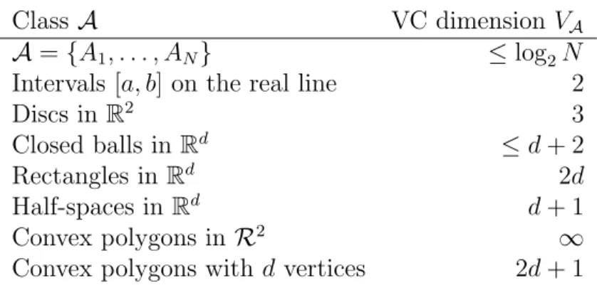
Class A VC dimension VA
A={A1, . . . , AN} ≤log2N
Intervals [a, b] on the real line 2
Discs in R2 3
Closed balls in Rd ≤d+ 2
Rectangles in Rd 2d
Half-spaces in Rd d+ 1 Convex polygons in R2 ∞ Convex polygons with d vertices 2d+ 1
Table 1: The VC dimension of some classes A.
Theorem 5 Let A be a class of sets. Then
P sup A∈A| Pn(A)−P(A)|> ≤8 sn(A) e−n 2/32 . (1)
This partly solves one of our problems. But, how big cansn(A) be? Sometimes sn(A) = 2n for all n. For example, let A be all polygons in the plane. Then s
n(A) = 2n for all n. But, in many cases, we will see that sn(A) = 2n for all n up to some integer d and then
sn(A)<2n for all n > d.
The Vapnik-Chervonenkis (VC) dimension is
d=d(A) = largest n such that sn(A) = 2n.
In other words, d is the size of the largest set that can be shattered.
Thus, sn(A) = 2n for all n ≤ d and sn(A) < 2n for all n > d. The VC dimensions of some common examples are summarized in Table 1. Now here is an interesting question: for
n > d how does sn(A) behave? It is less than 2n but how much less?
Theorem 6 (Sauer’s Theorem) Suppose that A has finite VC dimension d. Then, for all n≥d,
We conclude that:
Theorem 7 Let A be a class of sets with VC dimension d <∞. Then
P sup A∈A| Pn(A)−P(A)|> ≤8 (n+ 1)d e−n2/32. (3)
Example 8 Let’s return to our first example. Suppose that X1, . . . , Xn have cdf F. Let
Fn(t) = 1 n n X i=1 I(Xi ≤t).
We would like to bound P(supt|Fn(t)−F(t)| > ). Notice that Fn(t) = Pn(A) where A = (−∞, t]. Let A ={(−∞, t] : t ∈R}. This has VC dimension d = 1. So
P(sup t |Fn(t)−F(t)|> ) = P sup A∈A|Pn(A)−P(A)|> ≤8 (n+ 1) e−n2/32.
In fact, there is a tighter bound in this case called the DKW (Dvoretsky-Kiefer-Wolfowitz) inequality: P(sup t |Fn(t)−F(t)|> )≤2e −2n2 .
4
Bounding Expectations
Eearlier we saw that we can use exponential bounds on probabilities to get bounds on expectations. Let us recall how that works.
Consider a finite collection A={A1, . . . , AN}. Let
Zn = max 1≤j≤N|Pn(Aj)−P(Aj)|. We know that P(Zn > )≤2me−2n 2 . (4)
But now we want to bound
E(Zn) =
max |Pn(Aj)−P(Aj)|
Hence, for any s, E(Zn2) = Z ∞ 0 P (Zn2 > t)dt = Z s 0 P (Zn2 > t)dt+ Z ∞ s P (Zn2 > t)dt ≤ s+ Z ∞ s P (Zn2 > t)dt ≤ s+ 2N Z ∞ s e−2ntdt = s+ 2N e−2ns 2n = s+N ne −2ns. Lets = log(N)/(2n). Then
E(Zn2)≤s+N ne −2ns = logN 2n + 1 n = logN + 2 2n .
Finally, we use Cauchy-Schwartz:
E(Zn)≤ p E(Z2 n)≤ r logN + 2 2n =O r logN n ! . In summary: E max 1≤j≤N|Pn(Aj)−P(Aj)| =O r logN n ! .
For a single set A we would have E|Pn(A)−P(A)| ≤ O(1/√n). The bound only increases logarithmically withN.
Lecture Notes 4
1
Random Samples
LetX1, . . . , Xn ∼F. Astatistic is any functionT =g(X1, . . . , Xn). Recall that the sample mean is Xn = 1 n n X i=1 Xi
and sample variance is
Sn2 = 1 n−1 n X i=1 (Xi−Xn)2. Letµ=E(Xi) and σ2 =Var(Xi). Recall that
E(Xn) =µ, Var(Xn) = σ2 n , E(S 2 n) = σ2. Theorem 1 If X1, . . . , Xn ∼N(µ, σ2) then Xn∼N(µ, σ2/n).
Proof. We know that
MXi(s) =e µs+σ2s2/2 . So, MXn(t) = E(etXn) =E(ent Pni=1Xi) = (EetXi/n)n= (M Xi(t/n)) n=e(µt/n)+σ2t2/(2n2)n = exp ( µt+ σ2 nt 2 2 ) which is the mgf of aN(µ, σ2/n).
Example 2 (Example 5.2.10). Let Z1, . . . , Zn ∼Cauchy(0,1). Then Zn∼Cauchy(0,1).
2
Convergence
Let X1, X2, . . . be a sequence of random variables and let X be another random variable.
LetFn denote the cdf of Xn and letF denote the cdf ofX. 1. Xn converges almost surely to X, written Xn
a.s.
→ X, if, for every >0,
P( lim
n→∞|Xn−X|< ) = 1. (1)
2. Xn converges to X in probability, written Xn P
→X, if, for every >0,
P(|Xn−X|> )→0 (2)
asn → ∞. In other words,Xn−X =oP(1).
3. Xn converges to X in quadratic mean (also called convergence in L2), written
Xn
qm →X, if
E(Xn−X)2 →0 (3)
asn → ∞.
4. Xn converges to X in distribution, written Xn X, if lim
n→∞Fn(t) = F(t) (4)
at all t for which F is continuous.
Convergence to a Constant. A random variable X has a point mass distribution if there exists a constant c such that P(X = c) = 1. The distribution for X is denoted by δc and we writeX ∼δc. If Xn
P
→δc then we also write Xn P
→c. Similarly for the other types of convergence.
Theorem 4 Xn as
→X if and only if, for every >0, lim
n→∞P(supm≥n|Xm−X| ≤) = 1.
Example 5 (Example 5.5.8). This example shows that convergence in probabilitydoes not
imply almost sure convergence. Let S = [0,1]. Let P be uniform on [0,1]. We draw S ∼P. Let X(s) = s and let
X1 =s+I[0,1](s), X2 =s+I[0,1/2](s), X3 =s+I[1/2,1](s)
X4 =s+I[0,1/3](s), X5 =s+I[1/3,2/3](s), X6 =s+I[2/3,1](s)
Example 6 Let Xn ∼N(0,1/n). Intuitively, Xn is concentrating at 0 so we would like to say that Xn converges to 0. Let’s see if this is true. Let F be the distribution function for a point mass at 0. Note that √nXn ∼ N(0,1). Let Z denote a standard normal random variable. For t <0,
Fn(t) =P(Xn < t) =P(√nXn <√nt) =P(Z <√nt)→0 since √nt→ −∞. For t >0,
Fn(t) =P(Xn < t) =P(√nXn <√nt) =P(Z <√nt)→1
since √nt → ∞. Hence, Fn(t) → F(t) for all t 6= 0 and so Xn 0. Notice that Fn(0) = 1/2 6= F(1/2) = 1 so convergence fails at t = 0. That doesn’t matter because t = 0 is not a continuity point of F and the definition of convergence in distribution only requires convergence at continuity points.
Now consider convergence in probability. For any >0, using Markov’s inequality,
P(|Xn|> ) = P(|Xn|2 > 2)≤ E (X2 n) 2 = 1 n 2 →0 as n → ∞. Hence, Xn→P 0.
The next theorem gives the relationship between the types of convergence.
Theorem 7 The following relationships hold: (a) Xn qm →X implies that Xn P →X. (b) Xn P →X implies that Xn X.
(c) If Xn X and if P(X =c) = 1 for some real number c, then Xn P →X. (d) Xn as →X implies Xn P →X.
In general, none of the reverse implications hold except the special case in (c).
Proof. We start by proving (a). Suppose that Xn qm
→ X. Fix > 0. Then, using Markov’s inequality,
Also,
F(x−) = P(X ≤x−) = P(X≤x−, Xn≤x) +P(X≤x−, Xn> x)
≤ Fn(x) +P(|Xn−X|> ). Hence,
F(x−) − P(|Xn−X|> )≤Fn(x)≤F(x+) + P(|Xn−X|> ). Take the limit as n → ∞to conclude that
F(x−)≤lim inf
n→∞ Fn(x)≤lim supn→∞
Fn(x)≤F(x+).
This holds for all >0. Take the limit as →0 and use the fact that F is continuous at x
and conclude that limnFn(x) =F(x). Proof of (c). Fix >0. Then,
P(|Xn−c|> ) = P(Xn< c−) +P(Xn> c+)
≤ P(Xn≤c−) +P(Xn > c+)
= Fn(c−) + 1−Fn(c+) → F(c−) + 1−F(c+)
= 0 + 1−1 = 0.
Proof of (d). This follows from Theorem 4.
Let us now show that the reverse implications do not hold.
Convergence in probability does not imply convergence in quadratic mean. LetU ∼Unif(0,1) and letXn =√nI(0,1/n)(U). Then P(|Xn|> ) =P(√nI(0,1/n)(U)> ) =P(0≤U <1/n) = 1/n→0. Hence, Xn
P
→0. But E(X2 n) = n
R1/n
0 du = 1 for all n soXn does not converge in quadratic mean.
Convergence in distribution does not imply convergence in probability. Let X ∼ N(0,1).
Let Xn = −X for n = 1,2,3, . . .; hence Xn ∼ N(0,1). Xn has the same distribution
function as X for all n so, trivially, limnFn(x) = F(x) for all x. Therefore, Xn X. But
P(|Xn −X| > ) = P(|2X| > ) = P(|X| > /2) 6= 0. So Xn does not converge to X in
probability.
The relationships between the types of convergence can be summarized as follows:
q.m.
Example 8 One might conjecture that if Xn P
→ b, then E(Xn) → b. This is not true. Let Xn be a random variable defined by P(Xn = n2) = 1/n and P(Xn = 0) = 1−(1/n).
Now, P(|Xn| < ) = P(Xn = 0) = 1−(1/n) → 1. Hence, Xn
P
→ 0. However, E(Xn) = [n2×(1/n)] + [0×(1−(1/n))] = n. Thus, E(X
n)→ ∞.
Example 9 Let X1, . . . , Xn ∼ Uniform(0,1). Let X(n) = maxiXi. First we claim that
X(n) P
→1. This follows since
P(|X(n)−1|> ) =P(X(n) ≤1−) = Y i P(Xi ≤1−) = (1−)n →0. Also P(n(1−X(n))≤t) =P(X(n) ≤1−(t/n)) = (1−t/n)n →e−t. So n(1−X(n)) Exp(1).
Some convergence properties are preserved under transformations.
Theorem 10 Let Xn, X, Yn, Y be random variables. Let g be a continuous function. (a) If Xn→P X and Yn→P Y, then Xn+Yn→P X+Y.
(b) If Xn qm →X and Yn qm →Y, then Xn+Yn qm →X+Y. (c) If Xn X and Yn c, then Xn+Yn X+c. (d) If Xn P →X and Yn P →Y, then XnYn P →XY. (e) If Xn X and Yn c, then XnYn cX. (f ) If Xn P →X, then g(Xn) P →g(X). (g) If Xn X, then g(Xn) g(X).
• Parts (c) and (e) are know as Slutzky’s theorem
• Parts (f) and (g) are known as The Continuous Mapping Theorem.
• It is worth noting thatXn X andYn Y does not in general imply thatXn+Yn
Theorem 11 (The Weak Law of Large Numbers (WLLN))
If X1, . . . , Xn are iid, then Xn P
→µ. Thus, Xn−µ=oP(1).
Interpretation of the WLLN: The distribution of Xn becomes more concentrated aroundµ as n gets large.
Proof. Assume that σ < ∞. This is not necessary but it simplifies the proof. Using Chebyshev’s inequality, P |Xn−µ|> ≤ Var(Xn) 2 = σ2 n2 which tends to 0 as n→ ∞.
Theorem 12 The Strong Law of Large Numbers. Let X1, . . . , Xn be iid with mean µ. Then Xn
as →µ.
The proof is beyond the scope of this course.
4
The Central Limit Theorem
The law of large numbers says that the distribution ofXn piles up nearµ. This isn’t enough to help us approximate probability statements aboutXn. For this we need the central limit theorem.
Suppose that X1, . . . , Xn are iid with mean µ and variance σ2. The central limit the-orem (CLT) says that Xn = n−1PiXi has a distribution which is approximately Normal with mean µ and variance σ2/n. This is remarkable since nothing is assumed about the distribution of Xi, except the existence of the mean and variance.
Theorem 13 (The Central Limit Theorem (CLT)) LetX1, . . . , Xn be iid with meanµ and variance σ2. Let X
n=n−1Pni=1Xi. Then Zn ≡ Xn−µ q Var(Xn) = √ n(Xn−µ) σ Z
where Z ∼N(0,1). In other words, lim n→∞P(Zn≤z) = Φ(z) = Z z −∞ 1 √ 2πe −x2/2 dx.
Interpretation: Probability statements about Xn can be approximated using a Nor-mal distribution. It’s the probability statements that we are approximating, not the random variable itself.
A consequence of the CLT is that Xn−µ=OP r 1 n ! .
In addition to Zn N(0,1), there are several forms of notation to denote the fact that the distribution of Zn is converging to a Normal. They all mean the same thing. Here they are: Zn ≈ N(0,1) Xn ≈ N µ, σ 2 n Xn−µ ≈ N 0, σ 2 n √ n(Xn−µ) ≈ N 0, σ2 √ n(Xn−µ) σ ≈ N(0,1).
Recall that if X is a random variable, its moment generating function (mgf) is ψX(t) =
EetX. Assume in what follows that the mgf is finite in a neighborhood around t= 0.
Lemma 14 Let Z1, Z2, . . . be a sequence of random variables. Let ψn be the mgf of Zn. Let
Z be another random variable and denote its mgf by ψ. If ψn(t) → ψ(t) for all t in some open interval around 0, then Zn Z.
Proof of the central limit theorem. Let Yi = (Xi −µ)/σ. Then, Zn =n−1/2PiYi. Letψ(t) be the mgf of Yi. The mgf of PiYi is (ψ(t))n and mgf ofZn is [ψ(t/√n)]n≡ξn(t). Now ψ0(0) =E(Y 1) = 0, ψ00(0) =E(Y12) =Var(Y1) = 1. So, ψ(t) = ψ(0) +tψ0(0) + t 2 2!ψ 00(0) + t3 3!ψ 000(0) +· · · = 1 + 0 + t 2 2 + t3 3!ψ 000(0) +· · · = 1 + t 2 2 + t3 3!ψ 000(0) +· · · Now,
which is the mgf of a N(0,1). The result follows from Lemma 14. In the last step we used the fact that if an →a then
1 + an
n
n
→ea.
The central limit theorem tells us that Zn = √n(Xn −µ)/σ is approximately N(0,1). However, we rarely knowσ. We can estimate σ2 from X
1, . . . , Xn by Sn2 = 1 n−1 n X i=1 (Xi−Xn)2.
This raises the following question: if we replace σ with Sn, is the central limit theorem still true? The answer is yes.
Theorem 15 Assume the same conditions as the CLT. Then,
Tn =
√
n(Xn−µ)
Sn
N(0,1).
Proof. We have that
Tn =ZnWn where Zn = √ n(Xn−µ) σ and Wn = σ Sn . Now Zn N(0,1) andWn P
→1. The result follows from Slutzky’s theorem.
There is also a multivariate version of the central limit theorem. Recall that X =
(X1, . . . , Xk)T has a multivariate Normal distribution with mean vector µ and covariance
matrix Σ if f(x) = 1 (2π)k/2|Σ|1/2 exp −1 2(x−µ) TΣ−1(x−µ) .
In this case we write X ∼N(µ,Σ).
Theorem 16 (Multivariate central limit theorem) Let X1, . . . , Xn be iid random vec-tors where Xi = (X1i, . . . , Xki)T with meanµ= (µ1, . . . , µk)T and covariance matrix Σ. Let
X = (X1, . . . , Xk)T where Xj =n−1Pni=1Xji. Then, √
5
The Delta Method
IfYn has a limiting Normal distribution then the delta method allows us to find the limiting distribution of g(Yn) where g is any smooth function.
Theorem 17 (The Delta Method) Suppose that √
n(Yn−µ)
σ N(0,1)
and that g is a differentiable function such that g0(µ)6= 0. Then √ n(g(Yn)−g(µ)) |g0(µ)|σ N(0,1). In other words, Yn ≈N µ, σ2 n ! implies that g(Yn)≈N g(µ),(g0(µ))2 σ2 n ! .
Example 18 LetX1, . . . , Xn be iid with finite mean µand finite variance σ2. By the central limit theorem, √n(Xn − µ)/σ N(0,1). Let Wn = eXn. Thus, Wn = g(Xn) where
g(s) =es. Since g0(s) =es, the delta method implies that W
n ≈N(eµ, e2µσ2/n). There is also a multivariate version of the delta method.
Theorem 19 (The Multivariate Delta Method) Suppose that Yn = (Yn1, . . . , Ynk) is a sequence of random vectors such that
√
n(Yn−µ) N(0,Σ).
Let g :Rk →R and let
∇g(y) = ∂g ∂y1 ... ∂g ∂yk .
Let ∇µ denote ∇g(y) evaluated at y = µ and assume that the elements of ∇µ are nonzero. Then
and define Yn =X1X2. Thus, Yn = g(X1, X2) where g(s1, s2) = s1s2. By the central limit theorem, √ n X1−µ1 X2−µ2 N(0,Σ). Now ∇g(s) = ∂g ∂s1 ∂g ∂s2 ! = s2 s1 and so ∇T µΣ∇µ= (µ2 µ1) σ11 σ12 σ12 σ22 µ2 µ1 =µ22σ11 + 2µ1µ2σ12 + µ21σ22. Therefore, √ n(X1X2−µ1µ2) N 0, µ22σ11 + 2µ1µ2σ12 + µ21σ22 .
Addendum to Lecture Notes 4
Here is the proof thatTn= √ n(Xn−µ) Sn N(0,1) where Sn2 = 1 n−1 n X i=1 (Xi−Xn)2.
Step 1. We first show that R2 n P →σ2 where R2n = 1 n n X i=1 (Xi−Xn)2. Note that R2n= 1 n n X i=1 Xi2− 1 n n X i=1 Xi !2 .
DefineYi =Xi2. Then, using the LLN (law of large numbers) 1 n n X i=1 Xi2 = 1 n n X i=1 Yi P →E(Yi) =E(Xi2) =µ2+σ2. Next, by the LLN, 1 n n X i=1 Xi →P µ.
Since g(t) =t2 is continuous, the continuous mapping theorem implies that 1 n n X i=1 Xi !2 P →µ2. Thus R2n →P (µ2+σ2)−µ2 =σ2.
Step 4. Since g(t) = t/σ is continuous, the continuous mapping theorem implies that
Sn/σ P →1.
Step 5. Since g(t) = 1/t is continuous (for t > 0) the continuous mapping theorem implies thatσ/Sn
P
→1. Since convergence in probability implies convergence in distribution,
σ/Sn 1.
Step 5. Note that
Tn= √ n(Xn−µ) σ σ Sn ≡VnWn.
Now Vn Z where Z ∼ N(0,1) by the CLT. And we showed that Wn 1. By Slutzky’s theorem, Tn =VnWn Z×1 = Z.
Lecture Notes 5
1
Statistical Models
A statistical modelP is a collection of probability distributions (or a collection of densities). An example of a nonparametric modelis
P = ( p: Z (p00(x))2dx <∞ ) .
A parametric model has the form
P =
(
p(x;θ) : θ∈Θ
)
where Θ ⊂ Rd. An example is the set of Normal densities {p(x;θ) = (2π)−1/2e−(x−θ)2/2
}. For now, we focus on parametric models.
The model comes from assumptions. Some examples:
• Time until something fails is often modeled by an exponential distribution. • Number of rare events is often modeled by a Poisson distribution.
• Lengths and weights are often modeled by a Normal distribution.
These models are not correct. But they might be useful. Later we consider nonpara-metric methods that do not assume a paranonpara-metric model
• sample mean: X = 1 n P iXi, • sample variance: S2 = 1 n−1 P i(Xi−x)2,
• sample median: middle value of ordered statistics, • sample minimum: X(1)
• sample maximum: X(n) • sample range: X(n)−X(1)
• sample interquartile range: X(.75n)−X(.25n)
Example 1 If X1, . . . , Xn∼Γ(α, β), then X ∼Γ(nα, β/n). Proof: MX = E[etx] =E[ePXit/n] =Y i E[eXi(t/n)] = [MX(t/n)]n= 1 1−βt/n αn = 1 1−β/nt nα . This is the mgf of Γ(nα, β/n). Example 2 If X1, . . . , Xn∼N(µ, σ2) then X ∼N(µ, σ2/n).
Example 3 If X1, . . . , Xn iid Cauchy(0,1),
p(x) = 1
π(1 +x2) for x∈R, then X ∼ Cauchy(0,1).
Example 4 If X1, . . . , Xn∼N(µ, σ2) then (n−1)
σ2 S
2 ∼χ2 (n−1). The proof is based on the mgf.
Example 5 Let X(1), X(2), . . . , X(n) be the order statistics, which means that the sample
X1, X2, . . . , Xn has been ordered from smallest to largest:
X(1) ≤X(2) ≤ · · · ≤X(n). Now,
FX(k)(x) = P(X(k) ≤x)
= P(at least k of the X1, . . . , Xn ≤x) = n X j=k P(exactly j of theX1, . . . , Xn≤x) = n X j=k n j [FX(x)]j[1−FX(x)]n−j
Differentiate to find the pdf (See CB p. 229):
pX(k)(x) = n! (k−1)!(n−k)![FX(x)] k−1 p(x) [1 −FX(x)]n−k.
3
Sufficiency
(Ch 6 CB) We continue with parametric inference. In this section we discuss data reductionas a formal concept.
• SampleXn =X
1,· · · , Xn ∼F.
3.1
Sufficient Statistics
Definition: T is sufficient for θ if the conditional distribution of Xn|T does not depend on
θ. Thus, f(x1, . . . , xn|t;θ) =f(x1, . . . , xn|t).
Example 6 X1,· · ·, Xn∼Poisson(θ). Let T =Pni=1Xi. Then,
pXn|T(xn|t) =P(Xn=xn|T(Xn) = t) = P(X n =xn and T =t) P(T =t) . But P(Xn =xn and T =t) = 0 if T(xn)6=t P(Xn =xn) if T(Xn) = t Hence, P(Xn =xn) = n Y i=1 e−θθxi xi! = e− nθθP xi Q (xi!) = e− nθθt Q (xi!) . Now, T(xn) = Px i =t and so P(T =t) = e −nθ(nθ)t t! since T ∼Poisson(nθ). Thus, P(Xn =xn) P(T =t) = t! (Qxi)!nt
which does not depend on θ. So T = PiXi is a sufficient statistic for θ. Other sufficient statistics are: T = 3.7PiXi, T = (PiXi, X4), and T(X1, . . . , Xn) = (X1, . . . , Xn).
3.2
Sufficient Partitions
It is better to describe sufficiency in terms of partitions of the sample space.
xn t p(x|t) (0, 0, 0) → t= 0 1 (0, 0, 1) → t= 1 1/3 (0, 1, 0) → t= 1 1/3 (1, 0, 0) → t= 1 1/3 (0, 1, 1) → t= 2 1/3 (1, 0, 1) → t= 2 1/3 (1, 1, 0) → t= 2 1/3 (1, 1, 1) → t= 3 1 8 elements → 4 elements
1. A partition B1, . . . , Bk is sufficient iff(x|X ∈B) does not depend on θ.
2. A statistic T induces a partition. For each t, {x : T(x) = t} is one element of the partition. T is sufficient if and only if the partition is sufficient.
3. Two statistics can generate the same partition: example: PiXi and 3PiXi.
4. If we split any element Bi of a sufficient partition into smaller pieces, we get another sufficient partition.
Example 8 Let X1, X2, X3 ∼ Bernoulli(θ). Then T = X1 is not sufficient. Look at its partition:
xn t p(x|t) (0, 0, 0) → t= 0 (1−θ)2 (0, 0, 1) → t= 0 θ(1−θ) (0, 1, 0) → t= 0 θ(1−θ) (0, 1, 1) → t= 0 θ2 (1, 0, 0) → t= 1 (1−θ)2 (1, 0, 1) → t= 1 θ(1−θ) (1, 1, 0) → t= 1 θ(1−θ) (1, 1, 1) → t= 1 θ2 8 elements → 2 elements
3.3
The Factorization Theorem
Theorem 9 T(Xn) is sufficient for θ if the joint pdf/pmf of Xn can be factored as
p(xn;θ) =h(xn)×g(t;θ).
Example 10 Let X1,· · · , Xn ∼Poisson. Then
p(xn;θ) = e −nθθP Xi Q (xi!) = Q1 (xi!)× e−nθθPiXi. Example 11 X1,· · · , Xn∼N(µ, σ2). Then p(xn;µ, σ2) = 1 2πσ2 n 2 exp − P (xi−x)2 +n(x−µ)2 2σ2 . (a) If σ known: p(xn;µ) = 1 2πσ2 n 2 exp −P(xi−x)2 2σ2 | {z } h(xn) exp −n(x−µ)2 2σ2 | {z } g(T(xn)|µ) .
Thus, X is sufficient for µ.
(b) If (µ, σ2) unknown then T = (X, S2) is sufficient. So is T = (PX
3.4
Minimal Sufficient Statistics (MSS)
We want the greatest reduction in dimension.Example 12 X1,· · · , Xn∼N(0, σ2). Some sufficient statistics are:
T(X1,· · · , Xn) = (X1,· · ·, Xn) T(X1,· · · , Xn) = (X12,· · · , Xn2) T(X1,· · · , Xn) = m X i=1 Xi2, n X i=m+1 Xi2 ! T(X1,· · · , Xn) = X Xi2.
Definition: T is aMinimal Sufficient Statistic if the following two statements are true: 1. T is sufficient and
2. If U is any other sufficient statistic then T =g(U) for some function g. In other words, T generates thecoarsest sufficient partition.
SupposeU is sufficient. SupposeT =H(U) is also sufficient. T provides greater reduction than U unless H is a 1−1 transformation, in which case T and U are equivalent.
Example 13 X ∼ N(0, σ2). X is sufficient. |X| is sufficient. |X| is MSS. So are
X2, X4, eX2
.
xn t p(x|t) u p(x|u) (0, 0, 0) → t = 0 1 u= 0 1 (0, 0, 1) → t = 1 1/3 u= 1 1/3 (0, 1, 0) → t = 1 1/3 u= 1 1/3 (1, 0, 0) → t = 1 1/3 u= 1 1/3 (0, 1, 1) → t = 2 1/3 u= 73 1/2 (1, 0, 1) → t = 2 1/3 u= 73 1/2 (1, 1, 0) → t = 2 1/3 u= 91 1 (1, 1, 1) → t = 3 1 u= 103 1
Note that U and T are both sufficient but U is not minimal.
3.5
How to find a Minimal Sufficient Statistic
Theorem 15 Define
R(xn, yn;θ) = p(yn;θ)
p(xn;θ). Suppose that T has the following property:
R(xn, yn;θ) does not depend on θ if and only if T(yn) = T(xn). Then T is a MSS.
Example 16 Y1,· · · , Yn iid Poisson (θ).
p(yn;θ) = e−nθθ P yi Q yi , p(y n;θ) p(xn;θ) = θP yi−Pxi Q yi!/Qxi!
which is independent of θ iff Pyi = Pxi. This implies that T(Yn) = PYi is a minimal sufficient statistic for θ.
The minimal sufficient statistic is not unique. But, the minimal sufficient partition is unique.
Example 17 Cauchy. p(x;θ) = 1 π(1 + (x−θ)2). Then p(yn;θ) p(xn;θ) = n Q i=1{ 1 + (xi−θ)2} n Q j=1{ 1 + (yj −θ)2} .
The ratio is a constant function of θ if
T(Yn) = (Y(1),· · · , Y(n)).
It is technically harder to show that this is true only if T is the order statistics, but it could be done using theorems about polynomials. Having shown this, one can conclude that the order statistics are the minimal sufficient statistics for θ.
Lecture Notes 6
1
The Likelihood Function
Definition. Let Xn = (X
1,· · · , Xn) have joint density p(xn;θ) = p(x1, . . . , xn;θ) where
θ∈Θ. The likelihood functionL: Θ→[0,∞) is defined by
L(θ)≡L(θ;xn) =p(xn;θ) where xn is fixed and θ varies in Θ.
1. The likelihood function is a function of θ.
2. The likelihood function is not a probability density function. 3. If the data are iid then the likelihood is
L(θ) = n Y i=1
p(xi;θ) iid case only.
4. The likelihood is only defined up to a constant of proportionality.
5. The likelihood function is used (i) to generate estimators (the maximum likelihood estimator) and (ii) as a key ingredient in Bayesian inference.
Example 1 These 2 samples have the same likelihood function: (X1, X2, X3)∼Multinomial (n= 6, θ, θ,1−2θ) X = (1,3,2) =⇒ L(θ) = 6! 1!3!2!θ 1θ3(1−2θ)2 ∝θ4(1−2θ)2 X = (2,2,2) =⇒ L(θ) = 6! 2!2!2!θ 2θ2(1−2θ)2 ∝θ4(1−2θ)2 Example 2 X1,· · ·, Xn∼N(µ,1). Then, L(µ) = 1 2π n 2 exp ( −12 n X i=1 (xi −µ)2 ) ∝expn−n 2(x−µ) 2o.
Example 3 Let X1, . . . , Xn∼Bernoulli(p). Then
L(p)∝pX(1−p)n−X for p∈[0,1] where X =PiXi.
Theorem 4 Writexn ∼yn ifL(θ|xn)∝L(θ|yn). The partition induced by∼is the minimal sufficient partition.
Example 5 A non iid example. An AR(1) time series auto regressive model. The model is:
X1 ∼N(0, σ2) and
Xi+1 =θXi+ei+1 ei
iid
∼N(0, σ2).
It can be show that we have the Markov property: o(xn+1|xn, xn−1,· · · , x1) = p(xn+1|xn). The likelihood function is
L(θ) = p(xn;θ) = p(x1;θ)p(x2|x1;θ)· · ·p(xn|x1, . . . , xn−1;θ) = p(xn|xn−1;θ)p(xn−1|xn−2;θ)· · ·p(x2|x1;θ)p(x1;θ) = n Y i=1 1 √ 2πθexp −1 2θ2(xn+i−1−θxn−i) 2 .
2
Likelihood, Sufficiency and the Likelihood Principle
The likelihood function is a minimal sufficient statistic. That is, if we define the equivalence relation: xn∼yn whenL(θ;xn)∝L(θ;yn) then the resulting partition is minimal sufficient.LetS1, . . . , Sn ∼Bernoulli(π) where π is known. IfSi = 1 you get to see ci. Otherwise, you do not. (This is an example of survey sampling.) The likelihood function is
Y i
πSi(1−π)1−Si.
The unknown parameter does not appear in the likelihood. In fact, there are no unknown parameters in the likeli