The Rimini Centre for Economic Analysis
Legal address: Via Angherà, 22 – Head office: Via Patara, 3 - 47900 Rimini (RN) – Italy
WP 38-07
GABRIELE FIORENTINI
Universituy of Firenze, Italy
and
The Rimini Centre for Economic Analysis, Rimini, Italy
ENRIQUE SENTANA
CEMFI, Madrid, Spain
“ON THE EFFICIENCY AND CONSISTENCY
OF LIKELIHOOD ESTIMATION
IN MULTIVARIATE CONDITIONALLY
HETEROSKEDASTIC DYNAMIC REGRESSION
MODELS
”
Copyright belongs to the author. Small sections of the text, not exceeding three
paragraphs, can be used provided proper acknowledgement is given.
The
Rimini Centre for Economic Analysis
(RCEA) was established in March 2007.
RCEA is a private, non-profit organization dedicated to independent research in
Applied and Theoretical Economics and related fields. RCEA organizes seminars and
workshops, sponsors a general interest journal
The Review of Economic Analysis
,
and
organizes a biennial conference:
Small Open
Economies in the Globalized World
(SOEGW). Scientific work contributed by the RCEA Scholars is published in the
RCEA Working Papers series
.
The views expressed in this paper are those of the authors. No responsibility for them
should be attributed to the Rimini Centre for Economic Analysis.
On the efficiency and consistency of likelihood
estimation in multivariate conditionally
heteroskedastic dynamic regression models
∗Gabriele Fiorentini
Universit`a di Firenze, Viale Morgagni 59, I-50134 Firenze, Italy The Rimini Centre for Economic Analysis
<fi[email protected]fi.it> Enrique Sentana
CEMFI, Casado del Alisal 5, E-28014 Madrid, Spain
<sentana@cemfi.es> February 2003 Revised: July 2007
Abstract
We rank the efficiency of several likelihood-based parametric and semiparametric estima-tors of conditional mean and variance parameters in multivariate dynamic models withi.i.d.
spherical innovations, and show that Gaussian pseudo maximum likelihood estimators are inefficient except under normality. We also provide conditions for partial adaptivity of semi-parametric procedures, and relate them to the consistency of distributionally misspecified maximum likelihood estimators. We propose Hausman tests that compare Gaussian pseudo maximum likelihood estimators with more efficient but less robust competitors. We also study the efficiency of sequential estimators of the shape parameters. Finally, we provide finite sample results through Monte Carlo simulations.
Keywords: Adaptivity, ARCH, Elliptical Distributions, Financial Returns, Hausman tests, Semiparametric Estimators, Sequential Estimators.
JEL: C13, C14, C12, C51, C52
∗We would like to thank Dante Amengual, Manuel Arellano, Nour Meddahi, Javier Menc´ıa, Olivier Scaillet,
Paolo Zaffaroni, participants at the European Meeting of the Econometric Society (Stockholm, 2003), the Sympo-sium on Economic Analysis (Seville, 2003), the CAF Conference on Multivariate Modelling in Finance and Risk Management (Sandbjerg, 2006), the Second Italian Congress on Econometrics and Empirical Economics (Rimini, 2007), as well as audiences at AUEB, Bocconi, Cass Business School, CEMFI, CREST, EUI, Florence, NYU, RCEA, Roma La Sapienza and Queen Mary for useful comments and suggestions. Of course, the usual caveat applies.
1
Introduction
Many empirical studies with …nancial time series data indicate that the distribution of asset returns is usually rather leptokurtic, even after controlling for volatility clustering e¤ects. Nev-ertheless, the Gaussian pseudo-maximum likelihood (PML) estimators advocated by Bollerslev and Wooldridge (1992) remain consistent for the conditional mean and variance parameters in those circumstances, so long as those moments are correctly speci…ed.
However, a non-normal distribution may be indispensable when one is interested in features of the distribution of asset returns beyond its conditional mean and variance. For instance, empirical researchers and …nancial market practitioners are often interested in the so-called Value at Risk of an asset, which is the positive threshold valueV such that the probability of the asset su¤ering a reduction in wealth larger thanV equals some pre-speci…ed level{<1=2. In addition, they are sometimes interested in the probability of the joint occurrence of several extreme events, which is regularly underestimated by the multivariate normal distribution, especially in larger dimensions. This naturally leads one to specify a parametric leptokurtic distribution for the standardised innovations, such as the multivariate studenttanalysed in Fiorentini, Sentana and Calzolari (2003) (FSC), and to estimate the conditional mean and variance parameters jointly with the parameters characterising the shape of the assumed distribution by maximum likelihood (ML). However, while ML will often yield more e¢ cient estimators of the conditional mean and variance parameters than Gaussian PML if the assumed conditional distribution is correct, it may end up sacri…cing consistency when it is not, as shown by Newey and Steigerwald (1997).
If one were mostly interested in the …rst two conditional moments, the semiparametric (SP) estimators of Engle and Gonzalez-Rivera (1991) and Gonzalez-Rivera and Drost (1999) would o¤er an attractive solution because they are sometimes both consistent and partially e¢ cient, as proved by Linton (1993), Drost and Klaassen (1997), Drost, Klaassen and Werker (1997), or Sun and Stengos (2006). However, they su¤er from the curse of dimensionality, which severely limits their use in multivariate models. To avoid this problem, Hodgson and Vorkink (2003) and Hafner and Rombouts (2007) have recently discussed elliptically symmetric semiparametric (SSP) estimators, which retain univariate rates for their nonparametric part regardless of the cross-sectional dimension of the data, but which are unfortunately less robust.
One of the main objectives of our paper is to study in detail the trade-o¤s between e¢ ciency and consistency of the conditional mean and variance parameters that arise in this context. While many of the aforementioned papers provide detailed analyses of one of these issues, es-pecially in univariate models, or in models with no mean, to our knowledge we are the …rst to simultaneously analyse all the hard choices than an empirical researcher faces in practice.
Fur-thermore, we do so in a multivariate framework with non-zero means, in which some of the earlier results seem misleadingly simple. Moreover, we explicitly look at the e¢ ciency ranking of the feasible ML procedure that jointly estimates the shape parameters, as well as the infeasible ML, SSP, SP and PML estimators considered in the existing literature. We also provide conditions for partial adaptivity of the SSP and SP procedures, which we relate to the conditions for the consistency of the corresponding parametric ML estimators when the conditional distribution is misspeci…ed. Finally, we propose simple Hausman tests that compare the feasible ML and SSP estimators to the Gaussian PML ones to assess the validity of the distributional assumptions.
But given that practitioners often want to go beyond the …rst two conditional moments, one cannot simply treat the shape parameters as nuisance parameters. For that reason, we also consider sequential estimators of the shape parameters, which can be easily obtained from the standardised innovations evaluated at the Gaussian PML estimators, and assess their asymptotic e¢ ciency relative to their feasible ML counterpart. In particular, we consider a sequential ML estimator, as well as sequential method of moments (MM) estimators based on higher order moment parameters such as the coe¢ cient of multivariate excess kurtosis.
The rest of the paper is organised as follows. In section 2, we present closed-form ex-pressions for the score vector, Hessian and conditional information matrices of a log-likelihood function based on a spherically symmetric assumption for the innovations, and derive the e¢ -ciency bounds of the Gaussian PML estimator and both SP estimators, as well as the sequential estimators of the shape parameters. Then, in section 3 we compare the e¢ ciency of the di¤erent estimators of the conditional mean and variance parameters, discuss two speci…c models of prac-tical interest, and obtain some general results on partial adaptivity. In section 4, we compare the relative e¢ ciency of the di¤erent estimators of the shape parameters, while in section 5 we …rst study the consistency of the conditional mean parameters when the conditional distribution is misspeci…ed, and then introduce the Hausman tests. A Monte Carlo evaluation of the di¤erent parameter estimators and testing procedures can be found in section 6. Finally, we present our conclusions in section 7. Proofs and auxiliary results are gathered in appendices.
2
Theoretical background
2.1 The model
In a multivariate dynamic regression model with time-varying variances and covariances, the vector of N dependent variables, yt, is typically assumed to be generated as:
yt= t( 0) + t1=2( 0)"t; t( ) = (zt; It 1; );
where () and vech[ ()] are N 1 and N(N + 1)=2 1 vector functions known up to the
p 1vector of true parameter values 0,ztare kcontemporaneous conditioning variables, It 1
denotes the information set available att 1, which contains past values ofytandzt,
1=2
t ( )is some particular “square root”matrix such that t1=2( ) t1=20( ) = t( ), and"t is a martingale di¤erence sequence satisfying E("tjzt; It 1; 0) =0and V("tjzt; It 1; 0) =IN. Hence,
E(ytjzt; It 1; 0) = t( 0)
V(ytjzt; It 1; 0) = t( 0)
: (1)
To complete the model, we need to specify the conditional distribution of "t. We shall initially assume that, conditional on zt and It 1,"t is independent and identically distributed as some particular member of the spherical family with a well de…ned density (see Appendix A), or"tjzt; It 1; 0; 0 i:i:d: s(0;IN; 0)for short, where are someq additional parameters
that determine the shape of the distribution of &t="t0"t. The most prominent example is the spherical normal distribution, which we denote by 0 = 0. For illustrative purposes, though, we shall also look in some detail at the special case of a standardised multivariate t with 0
degrees of freedom, or i:i:d: t(0;IN; 0) for short. As is well known, the multivariate studentt
approaches the multivariate normal as 0 ! 1, but has generally fatter tails. For that reason,
we de…ne as1= , which will always remain in the …nite range [0;1=2)under our assumptions.
2.2 The log-likelihood function, its score, Hessian and information matrix
Let = ( 0; )0 denote the p+q parameters of interest, which we assume variation free. Ignoring initial conditions, the log-likelihood function of a sample of size T based on a par-ticular parametric spherical assumption will take the form LT( ) = PTt=1lt( ), with lt( ) =
dt( ) +c( ) +g[&t( ); ], where dt( ) = 1=2 lnj t( )j corresponds to the Jacobian, c( ) to the constant of integration of the assumed density, and g[&t( ); ] to its kernel, where
&t( ) ="t0( )"t( ), "t( ) =
1=2
t ( )"t( ) and "t( ) =yt t( ). FSC provide expressions forc( )andg[&t( ); ]in the multivariate studenttcase, which are obviously such thatLT( ;0) collapses to a conditionally Gaussian log-likelihood.
Let st( ) denote the score function@lt( )=@ , and partition it into two blocks, s t( ) and
s t( ), whose dimensions conform to those of and , respectively. Then, it is straightforward to show that if t( ) has full rank, and t( ), t( ),c( )and g[&t( ); ]are di¤erentiable
s t( ) = @dt( ) @ + @g[&t( ); ] @& @&t( ) @ = [Zlt( );Zst( )] elt( ) est( ) =Zdt( )edt( ); (2) s t( ) = @c( )=@ +@g[&t( ); ]=@ =ert( ); (3) where @dt( )=@ = Zst( )vec(IN) @&t( )=@ = 2fZlt( )"t( ) +Zst( )vec "t( )"t0( ) g; (4)
Zlt( ) = @ 0t( )=@ 1=20 t ( ); Zst( ) = 1 2@vec 0[ t( )]=@ [ t1=20( ) 1=20 t ( )]; elt( ; ) = [&t( ); ] "t( ); (5) est( ; ) = vec [&t( ); ] "t( )"t0( ) IN ; (6)
[&t( ); ] = 2@g[&t( ); ]=@&; (7)
and @ t( )=@ 0 and @vec[ t( )]=@ 0 depend on the particular speci…cation adopted.1
Given that [&t( ); ]is equal to (N + 1)=[1 2 + &t( )] in the student tcase, and to 1 under Gaussianity, it is straightforward to check that s t( ; ) coincides with the expression in FSC, while s t( ;0)reduces to the multivariate normal expression in Bollerslev and Wooldridge (1992), in which case: edt( ;0) = elt ( ;0) est( ;0) = "t( ) vec["t( )"t0( ) IN] :
As for ert( ;0), FSC show that in the multivariate student t case it is proportional to the second generalised Laguerre polynomial:
ert( ;0) =&2t( )=4 (N + 2)&t( )=2 +N(N + 2)=4:
Letht( )denote the Hessian function@st( )=@ 0 =@2lt( )=@ @ 0. Assuming twice di¤er-entiability of the di¤erent functions involved, we will have
h t( ) = @2dt( ) @ @ 0 + @2g[&t( ); ] (@&)2 @&t( ) @ @&t( ) @ 0 + @g[&t( ); ] @& @2&t( ) @ @ 0 (8)
h t( ) = @&t( )=@ @2g[&t( ); ]=@&@ 0; (9)
h t( ) = @2c( )=@ @ 0+@2g[&t( ); ]=@ @ 0; where @2dt( )=@ @ 0= 2Zst( )Z0st( ) 1 2 vec 0 1 t ( ) Ip @vec @vec0[ t( )]=@ =@ 0; (10) @2&t( )=@ @ 0= 2Zlt( )Z0lt( ) + 8Zst( )[IN "t( )"t0( )]Z0st( ) + 4Zlt( )["t0( ) IN]Z0st( ) +4Zst( )["t( ) IN]Z0lt( ) 2["t0( ) 1=20 t ( ) Ip]@vec[@ 0t( )=@ ]@ 0
fvec0[ t1=2( )"t( )"t0( ) t1=20( )] Ipg@vecf@vec0[ t( )]=@ g=@ 0;
and @2g(&; )=(@&)2, @2g(&; )=@&@ 0 and @g(&; )=@ @ 0 depend on the speci…c distribution assumed for estimation purposes (see FSC for the multivariate studentt).
1Note that while both
Zt( )andedt( )depend on the speci…c choice of square root matrix t1=2( ),s t( )
does not, a property that inherits fromlt( ). The same result is not generally true for non-elliptical distributions
(see Mencía and Sentana (2005)), in which case one should rede…neZst( )asf@vec0[ t1=2( )]=@ g[IN
1=20
t ( )],
Given correct speci…cation, the results in Crowder (1976) imply thatet( ) = [e0dt( );ert( )]0 evaluated at 0follows a vector martingale di¤erence, and therefore, the same is true of the score vectorst( ). His results also imply that, under suitable regularity conditions, which in particular require that 0 belongs to the interior of the parameter space, the asymptotic distribution of the feasible ML estimator will bepT(^T 0)!N 0;I 1( 0) , whereI( 0) =E[It( 0)j 0],
It( ) = V [st( )jzt; It 1; ] =Zt( )M( )Z0t( ) = E[ht( )jzt; It 1; ]; Zt( ) = Zdt( ) 0 0 Iq = Zlt( ) Zst( ) 0 0 0 Iq ; and M( ) =V [et( )j ].
The following result generalises Propositions 3 in Lange, Little and Taylor (1989), 1 in FSC and 5.2 in Hafner and Rombouts (2007):
Proposition 1 If "tjzt; It 1; is i:i:d: s(0;IN; ) with density exp[c( ) +g(&t; )], then
M( ) = 0 @ Mll ( ) 0 0 0 Mss( ) Msr( ) 0 M0sr( ) Mrr( ) 1 A; (11) Mll( ) =V[elt( )j ] =mll( )IN; (12) Mss( ) =V[est( )j ] =mss( ) (IN2 +KN N) + [mss( ) 1]vec(IN)vec0(IN); (13) Msr( ) =E[est( )e0rt( ) ] = E @est( )=@ 0 =vec(IN)msr( ); (14) Mrr( ) =V[ert( )j ] = E[@ert( )=@ 0 ]; mll( ) =E 2[&t( ); ] &t( ) N =E 2@ [&t( ); ] @& &t( ) N + [&t( ); ] ; mss( ) = N N+ 2 h 1 +V n [&t( ); ] &t N oi =E 2@ [&t( ); ] @& &2t( ) N(N + 2) + 1; msr( ) =E [&t( ); ] &t( ) N 1 e 0 rt( ) = E &t( ) N @ [&t( ); ] @ 0 ;
where Kmn is the commutation matrix of orders m and n. In the multivariate standardised student t case, in particular: mll( ) = (N + ) ( 2) (N + + 2); mss( ) = (N+ ) (N+ + 2); msr( ) = 2 (N + 2) 2 ( 2) (N+ ) (N + + 2); Mrr( ) = 4 4 0 2 0 N + 2 N 4 2+N( 4) 8 2 ( 2)2(N + ) (N+ + 2);
where (:)is the di-gamma function (see Abramowitz and Stegun (1964)), which under normality reduce to 1, 1, 0 and N(N + 2)=2, respectively. In this sense, it is interesting to note that as
N increases, mll( ), mss( ) and msr( ) converge to /( -2), 1 and 0, respectively. This is due to the fact that the multivariate student tcan be written as a scale mixture of normals, with a positive mixing variable that can be …ltered out with increasing precision asN ! 1(see Mencía and Sentana (2005)). Thus, lt( ) will become arbitrarily close to the sum of the conditional
log-likelihood ofyt given the mixing variable, which is multivariate Gaussian and only depends on , plus the marginal of the mixing variable, which only depends on . Another point to note in relation to the studentt is thatmll( ) increases without bound as !2+ whilemss( ) remains bounded. This di¤erential behaviour is also characteristic of other leptokurtic elliptical distributions, such as the normal-gamma mixture, the Kotz distribution, or the Pearson type II.
2.3 Gaussian pseudo maximum likelihood estimators of
If the interest of the researcher lied exclusively in , which are the parameters characterising the conditional mean and variance functions, then one attractive possibility would be to estimate an equality restricted version of the model in which is set to zero. Let~T = arg max LT( ;0) denote such a PML estimator of . As we mentioned in the introduction, ~T remains
root-T consistent for 0 under correct speci…cation of t( ) and t( ) even though the conditional distribution of"tjzt; It 1; 0is not Gaussian, provided that it has bounded fourth moments. The
proof is based on the fact that in those circumstances, the pseudo log-likelihood score,s t( ;0), is a vector martingale di¤erence sequence when evaluated at 0, a property that inherits from
edt( ;0). Importantly, this property is preserved even when the standardised innovations, "t, are not stochastically independent of zt and It 1. The asymptotic distribution of the PML
estimator of is stated in the following result:2
Proposition 2 If "tjzt; It 1; 0 isi:i:d: s(0;IN; 0) with 0 <1, and the regularity conditions
A.1 in Bollerslev and Wooldridge (1992) are satis…ed, thenpT(~T 0)!N[0;C( 0)], where C( ) =A 1( )B( )A 1( ); A( ) = E[h t( ;0)j ] =E[At( )j ]; At( ) = E[h t( ;0)jzt; It 1; ] =Zdt( )K(0)Z0dt( ); B( ) =V [s t( ;0)j ] =E[Bt( )j ]; Bt( ) =V[s t( ;0)jzt; It 1; ] =Zdt( )K( )Z0dt( ); and K( ) =V[edt( ;0)jzt; It 1; ] = IN 0 0 ( +1) (IN2+KN N)+ vec(IN)vec0(IN) ; (15)
which only depends on through the population coe¢ cient of multivariate excess kurtosis
=E(&2tj )=[N(N + 2)] 1: (16)
But if 0 is in…nite thenB( 0)will be unbounded, and the asymptotic distribution of some
or all the elements of ~T will be non-standard, unlike that of^T (see Hall and Yao (2003)). The following result, which speci…es the covariance between the Gaussian pseudo score and the true score, will repeatedly prove useful below:
2Throughout this paper, we use the high level regularity conditions in Bollerslev and Wooldridge (1992) because
we want to leave unspeci…ed the conditional mean vector and covariance matrix in order to maintain full generality. Primitive conditions for speci…c multivariate models can be found for instance in Ling and McAleer (2003).
Proposition 3 If "tjzt; It 1; 0;%0 is i:i:d: (0;IN) with density function f("t;%), where % are
some shape parameters and %=0 denotes normality, then
E edt( ;0) edt0 ( ;%);e0rt( ;%) zt; It 1; ;% = [K(0)j0]: (17)
Note that (17) holds regardless of whether or not the conditional distribution of "t is spher-ical, provided we interpret ert( ) as the gradient with respect to the shape parameters%.
2.4 Sequential estimators of and
In practice, we will often be interested in features of the distribution of asset returns, such as its quantiles, which go beyond its conditional mean and variance. For that purpose, we can use ~T to obtain a sequential ML estimator of as ~T = arg max LT(~T; ), possibly subject to some inequality constraints on . In the studenttcase, for instance,~T will be characterised by the …rst-order Kuhn-Tucker (KT) conditions
s T(~T;~T) + ~ T = 0; ~T 0; ~ T 0; ~ T ~T = 0;
where s T( ; ) is the sample mean of s t( ; ), and the KT multiplier associated with the constraint 0.
Such a sequential ML estimator of can be given a rather intuitive interpretation. If 0were
known, then the squared Euclidean norm of the standardised innovations,&t( 0), would bei:i:d:
over time, with density function h(&; ).3 Therefore, we could obtain the infeasible ML estima-tor of by maximising with respect to the log-likelihood function of the observed &t( 0)0s,
PT
t=1lnh[&t( 0); ]. Although in practice the standardised residuals are usually unobservable,
it turns out that ~T is the estimator so obtained when we treat &t(~T) as if they were really observed.
The asymptotic distribution of the sequential ML estimator of , which re‡ects the sample uncertainty in ~T, is stated in the following result:
Proposition 4 If "tjzt; It 1; 0 isi:i:d: s(0;IN; 0) with 0 <1, and the regularity conditions
A.1 in Bollerslev and Wooldridge (1992) are satis…ed, then pT(~T 0)!N[0;F( 0)], where F( 0) =I 1( 0) +I 1( 0)I0 ( 0)C( 0)I ( 0)I 1( 0):
Importantly, since C( 0)will become unbounded as 0 ! 1, the asymptotic distribution of
~T will also be non-standard in that case, unlike that of the feasible ML estimator ^T.
If we can obtain closed-form expressions for at least q functions of&t, (:) say, then we can also compute a sequential method of moments (MM) estimator of , T( ) say, by minimising
3
For instance, when"tjzt; It 1; 0isi:i:d: t(0;IN; 0), the distribution of&twill be that of either anF variate
withN and 0 degrees of freedom multiplied by N( 0 2)= 0 if 0<1, or a chi-square random variable with N degrees of freedom under Gaussianity (see e.g. Lemma 1 in FSC).
with respect to the quadratic form n0T(~T; ) n T(~T; ), where is a positive de…nite weighting matrix, and n t( ; ) = [&t( )] Ef [&t( )]j g. Given that E[&t( )j ] =N, the most obvious moment to use is (16), which su¢ ces to identify in the multivariate student t
case through the theoretical relationship = 2=( 4)(see FSC). In this context, if we de…ne the in‡uence function
n t( ; ) = &2t( ) N(N+ 2) 1 2 1 4 ; we obtain T = max[0; T(~T)] 4 max[0; T(~T)] + 2 ; (18) where T(~T) = T 1PTt=1&2t(~T) N(N+ 2) 1
is Mardia’s (1970) sample coe¢ cient of multivariate excess kurtosis of the estimated standardised residuals. We can obtain a closely related estimator, T say, from the modi…ed in‡uence function
n t( ; ) = &2t( ) N(N + 2) 2(1 2 )&t( ) N(1 6 ) + (1 2 )2 (1 4 )(1 6 );
which is the relevant second-order orthogonal polynomial when &t is proportional to an FN; random variable. The asymptotic distributions of these two sequential MM estimators of are stated in the following result:
Proposition 5 If "tjzt; It 1; 0 is i:i:d: t(0;IN; 0), with 0 > 8, then under the regularity
conditions A.1 in Bollerslev and Wooldridge (1992) we have that pT( T 0) ! N[0;G( 0)]
and pT( T 0)!N[0;J( 0)], where G( 0) = [E( 0) +R0( 0)C( 0)R( 0) 2R0( 0)A 1( 0)D( 0)]=N2( 0); J( 0) = [L( 0) +Q0( 0)C( 0)Q( 0)]=N2( 0); D( 0) = cov[s t( 0;0); n t( 0; 0)j 0] = 4( 0 2)(N + 0 2) N( 0 4)( 0 6) Ws( 0); E( 0) = V[n t( 0; 0)j 0] = ( 0 2)2 ( 0 4)2 (N + 6)(N+ 4) N(N + 2) ( 0 2)( 0 4) ( 0 6)( 0 8) 1 ; L( 0) = V[n t( 0; 0)j 0] =E( 0) 8( 0 2)2(N+ 0 2) N( 0 6)2( 0 4) ; R( 0) = cov[s t( 0; 0); n t( 0; 0)j 0] = 4( 0 2) N( 0 4) Ws( 0); Q( 0) = cov[s t( 0; 0); n t( 0; 0)j 0] = 8( 0 2) N( 0 4)( 0 6) Ws( 0); N( 0) = cov[s t( 0; 0); n t( 0; 0)j 0] = 2 2 0 ( 0 4)2 ; and Ws( 0) =Zd( 0)[00; vec0(IN)]0=E[Zdt( 0)j 0][00; vec0(IN)]0 =E 1 2@vec 0[ t( 0)]=@ vec[ t1( 0)] 0 =E[Wst( 0)j 0] = Ef@dt( )=@ j 0g: (19)
Note that since both G( 0) and J( 0) will diverge to in…nity as 0 converges to 8 from
above, T and T will not be root-T consistent for 4 0 8. Moreover, since is in…nite for
2< 0 4, T and T will not even be consistent in the interior of this range.
More generally, we could consider the higher order moment parameters of spherical random variables introduced by Berkane and Bentler (1986), k( ), which Maruyama and Seo (2003) relate to the higher order moments of &t asE(&ktj ) = [ k( ) + 1]E(&ktj0), where
E(&ktj0) = 2k(N=2)(1 +N=2) (k 2 +N=2)(k 1 +N=2);
whence we can also obtain the higher-order orthogonal polynomials of &t.4 By using these additional moments, we can in principle improve the e¢ ciency of the sequential MM estimators, although the precision with which we can estimate k( ) rapidly decreases with k (see Newey and Powell (1998) for a characterisation of e¢ cient sequential estimators).
Finally, if we were to iterate the sequential ML procedure, and achieved convergence, then we would obtain fully e¢ cient ML estimators of all model parameters. In fact, a single scoring iteration without line searches that started from ~T and ~T (or any other root-T consistent estimators) would su¢ ce to yield an estimator of that would be asymptotically equivalent to the full-information ML estimator ^T, at least up to terms of orderOp(T 1=2). Speci…cally,
•T ~T •T ~T = I ( 0) I ( 0) I0 ( 0) I ( 0) 1 1 T T X t=1 s t(~T;~T) s t(~T;~T) :
If we use the partitioned inverse formula, then it is easy to see that
•T ~T = I ( 0) I ( 0)I 1( 0)I0 ( 0) 1 1 T T X t=1 h s t(~T;~T) I ( 0)I 1( 0)s t(~T;~T) i =I ( 0)1 T T X t=1 s j t(~T;~T); where I ( 0) = I ( 0) I ( 0)I 1( 0)I0 ( 0) 1; and s j t( 0; 0) = s t( 0; 0) I ( 0)I 1( 0)s t( 0; 0) = Zdt( 0)edt( 0) Ws( 0) msr( 0)Mrr1( 0)ert( 0) (20)
is the residual from the unconditional theoretical regression of the score corresponding to ,
s t( 0), on the score corresponding to ,s t( 0). The residual score s j t( 0; 0) is sometimes
4In the standardised multivariate studentt, for instance,
called the parametric e¢ cient score of , and its variance,
P( 0) =I ( 0) I ( 0)I 1( 0)I0 ( 0)
=I ( 0) Ws( 0)Ws0( 0) msr( 0)Mrr1( 0)m0sr( 0) ;
the marginal information matrix of , or the feasible parametric e¢ ciency bound. In this respect, note that I ( 0), which is the inverse ofP( 0), coincides with the …rst block ofI 1(
0), and
therefore it gives us the asymptotic variance of the feasible ML estimator,^T.
2.5 Semiparametric estimators of
It is worth noting that the last summand of (20) coincides withZd( 0)times the theoretical
least squares projection ofedt( 0)on (the linear span of)ert( 0), which is conditionally
orthog-onal to edt( 0;0) from Proposition 3. Such an interpretation immediately suggests alternative
estimators of that replace our parametric assumption on the shape of the distribution of the standardised innovations "t by nonparametric or semiparametric alternatives. In this section, we shall consider two such estimators.
The …rst one is fully nonparametric, and therefore replaces the linear span of ert( 0)by the
so-called unrestricted tangent set, which is the Hilbert space generated by all the time-invariant functions of "t with bounded second moments that have zero conditional means and are con-ditionally orthogonal toedt( 0;0). The following proposition, which generalises the univariate
results of Gonzalez-Rivera and Drost (1999) and Propositions 3 and 4 in Hafner and Rom-bouts (2007) to multivariate models in which the conditional mean vector is not identically zero, describes the resulting semiparametric e¢ cient score and the corresponding e¢ ciency bound:
Proposition 6 If "tjzt; It 1; 0;%0 is i:i:d: (0;IN) with density function f("t;%), where % are
some shape parameters and %=0 denotes normality, such that both its Fisher information matrix for location and scale
Mdd(%) =V [edt( ;%)jzt; It 1; ;%] =V elt( ;%) est( ;%) ;% =V @lnf["t( );%]=@" vecfIN +@lnf["t( );%]=@" "t0( )g ;% and the matrix of third and fourth order central moments
K(%) =V[edt( ;0)jzt; It 1; ;%] (21)
are bounded, then the semiparametric e¢ cient score will be given by:
Zdt( 0;%0)edt( 0;%0) Zd( 0;%0) edt( 0;%0) K(0)K+(%0)edt( 0;0) ; (22) while the semiparametric e¢ ciency bound is
S( 0) =I ( 0;%0) Zd( 0;%0) Mdd(%0) K(0)K+(%0)K(0) Z0d( 0;%0); (23) where + denotes Moore-Penrose inverses, and I ( ;%) =E Zdt( )Mdd(%)Z0dt( )j ;% :
In practice, however,f("t;%)has to be replaced by a nonparametric estimator, which su¤ers from the curse of dimensionality. For this reason, Hodgson and Vorkink (2001), Hafner and Rombouts (2007) and other authors have suggested to limit the admissible distributions to the class of spherically symmetric ones. As a consequence, the restricted tangent set in this case be-comes the Hilbert space generated by all time-invariant functions of&t( 0)with bounded second
moments that have zero conditional means and are conditionally orthogonal to edt( 0;0). The
following proposition, which corrects and extends Proposition 9 in Hafner and Rombouts (2007), provides the resulting elliptically symmetric semiparametric e¢ cient score and the corresponding e¢ ciency bound:
Proposition 7 When "tjzt; It 1; 0 is i:i:d: s(0;IN; 0) with 2=(N + 2) < 0 < 1, the
elliptically symmetric semiparametric e¢ cient score is given by:
s t( 0) =Zdt( 0)edt( 0) Ws( 0) [&t( 0); 0] &t( 0) N 1 2 (N+2) 0+2 &t( 0) N 1 ; (24)
while the elliptically symmetric semiparametric e¢ ciency bound is S( 0) =I ( 0) Ws( 0)W0s( 0) N + 2 N mss( 0) 1 4 N[(N + 2) 0+ 2] : (25)
Once again, edt( ) has to be replaced in practice by a semiparametric estimate obtained from the joint density of "t. However, the elliptical symmetry assumption allows us to obtain such an estimate from a nonparametric estimate of the univariate density of&t,h(&t; ), avoiding in this way the curse of dimensionality.
3
The relative e¢ ciency of the di¤erent estimators of
3.1 General ranking and full e¢ ciency conditions
In the previous section we have e¤ectively considered …ve di¤erent estimators of : (1) the infeasible ML estimator, whose computation requires knowledge of 0; (2) the feasible ML estimator, which simultaneously estimates ; (3) the elliptically symmetric semiparametric es-timator, which restricts "t to have an i:i:d: s(0;IN; ) conditional distribution, but does not impose any additional structure on the distribution of &t; (4) the unrestricted semiparametric estimator, which only assumes that the conditional distribution of"t isi:i:d:(0;IN); and (5) the Gaussian PML estimator, which imposes = 0 even though the true conditional distribution of "t may not be normal. The following proposition ranks (in the usual positive semide…nite sense) the “information matrices” of those …ve estimators:
Proposition 8 If "tjzt; It 1; 0 is i:i:d: s(0;IN; 0) with 0 <1, then
In general, the above matrix inequalities are strict, at least in part. However, there is one instance in which all the above inequalities become equalities: when the true conditional distribution is Gaussian. In that case, the PML estimator is obviously fully e¢ cient, which implies that all the other estimators of must also be e¢ cient. Moreover, normality is the only such instance within the spherical family:
Proposition 9 1. If"tjzt; It 1; 0 is i:i:d: N(0;IN), then
It( 0;0) =V [st( 0;0)jzt; It 1; 0;0] =
V [s t( 0;0)jzt; It 1; 0;0] 0
00 Mrr(0)
where
V [s t( 0;0)jzt; It 1; 0;0] = E[h t( 0;0)jzt; It 1; 0;0] =At( 0;0) =Bt( 0;0):
2. If "tjzt; It 1; 0 is i:i:d: s(0;IN; 0) with 2=(N + 2) < 0 < 1, and Ws( 0) 6= 0, then S( 0) =I ( 0) only if &tjzt; It 1; 0 is i:i:d: Gamma with mean N and variance
N[(N+ 2) 0+ 2].
3. If "tjzt; It 1; 0 is i:i:d: s(0;IN; 0) with 0 <1, andZl( 0)=6 0, then S( 0) =I ( 0) only if 0=0.
The …rst part of this proposition, which generalises Proposition 2 in FSC, implies that as far as is concerned, there is no asymptotic e¢ ciency loss in estimating when 0 = 0.5 The second part, which generalises the results in Gonzalez-Rivera (1997), implies that the SSP estimator can be fully e¢ cient only if "t has a conditional Kotz distribution (see Kotz (1975)), which is a su¢ cient but not necessary condition formsr( 0) =0, which in turn implies P( 0) = I ( 0). Finally, the last part of Proposition 9 generalises Result 2 in Drost and Gonzalez-Rivera (1999) and Proposition 6 in Hafner and Rombouts (2007).
Unfortunately, it is virtually impossible to obtain closed-form expressions for the di¤erent e¢ ciency bounds in dynamic conditionally heteroskedastic non-Gaussian models, as one has to resort to Monte Carlo integration methods to compute the expected values of Zdt( ) or
Zdt( )K( )Z0dt( ) (see e.g. Engle and Gonzalez-Rivera (1991) and Gonzalez-Rivera and Drost (1999)). In the next subsection, though, we shall obtain closed-form expressions in two situations of practical interest.
3.2 Examples
Univariate conditionally heteroskedastic autoregressive models:
Consider the following univariate, covariance stationary Ar(h)-Arch(q) model: 5
In the multivariate studenttcase, in fact, the feasible ML estimator of will be numerically identical to the PML estimator approximately half the time in large samples because = 0lies at the boundary of the admissible parameter space (see e.g. Andrews (1999)).
yt= t( 0; 0) + t( 0)"t; t( ; ) = (1 Ph j=1 j) + Ph j=1 jyt j; 2 t( ) = (1 Pq j=1 j) +Pqj=1 j[yt j t j( ; )]2; "tjzt; It 1; 0; 0 i:i:d: s(0;1; 0): 9 > > = > > ; (26)
De…ne = ( 1; : : : ; h)0 and = ( 1; : : : ; q)0, so that = ( ; 0; ; 0)0. We can establish the following result:
Proposition 10 If in model (26) 0 =0, and all the roots of 1 Phj=1 j0Lj = 0 are outside
the unit circle, then the feasible ML estimators of , and are as e¢ cient as the infeasible ML estimators, which require knowledge of 0. If in addition 0 < 1, then the elliptically symmetric semiparametric estimators of , and are also fully e¢ cient. The same is true of the semiparametric estimators of and , but not of . In contrast, the ine¢ ciency ratio of the Gaussian PML estimators is mll1( 0) for and , and 4=f[3mss( 0) 1](3 0+ 2)g for .
Not surprisingly, we can also show that these ine¢ ciency ratios coincide with the ratios of the non-centrality parameters of the corresponding tests of conditional homoskedasticity against local alternatives of the form 0T = 0=
p
T in model (26) (see Linton and Steigerwald (2000)).
Multivariate conditionally heteroskedastic autoregressive models:
Consider a single factor version of the conditionally heteroskedastic factor model in Sentana and Fiorentini (2001) augmented with covariance stationary diagonalVar(1) dynamics:
yt= t( 0; 0) + 1=2 t ( 0)"t; t( ; ) = [IN diag( )] +diag( )yt 1; t( ) =cc0 t( ) + ; t( ) = 1 +Pqj=1 j[fkt j2 ( ) +!t j( ) 1]; "tjzt; It 1; 0; 0 i:i:d: s(0;IN; 0); 9 > > > > > = > > > > > ; (27)
wherefkt( )is the conditionally linear Kalman …lter estimator of the underlying common factor, and !t( ) the corresponding conditional mean square error (see Sentana (2004) for details). De…ne = ( 1; : : : ; N)0, = ( 1; : : : ; N)0, = vecd( ), and = ( 1; : : : ; q)0, so that
= ( 0; 0;c0; 0; 0)0. We can establish the following result:
Proposition 11 If in model (27) 0 = 0, i0 > 0 8i, and j i0j < 1 8i, then the feasible ML
estimators of , and are as e¢ cient as the infeasible ML estimators, which require 0 to be known. If in addition 0 <1, then the elliptically symmetric semiparametric estimators of , and are also fully e¢ cient. The same is also true of the semiparametric estimators of and , but not of . In contrast, the ine¢ ciency ratio of the Gaussian PML estimators is
mll1( 0) for and , and4=f[3mss( 0) 1](3 0+ 2)g for .
These ine¢ ciency ratios coincide with the corresponding ratios in the univariate example of Proposition 10. In the multivariate student t case with 0 > 4, in particular, they become
( 0 2)( 0+N+ 2)=[ 0( 0+N)]and( 0+N+ 2) ( 0 4)=[( 0 1)( 0+N 1)], respectively.
0 ! 1in accordance to Proposition 9, and 0 from above as 0 !2+or 0 !4+. For instance,
for N = 1 and 0 = 9, they take the value of :93 and :83, respectively, while for 0 = 5, their
values are only:8and:4. At the same time, these ratios are decreasing inN for a given 0, which
re‡ects the fact that the information matrix is “increasing”inN, as discussed after Proposition 1. For 0 = 9and N = 3, for instance, they take the value of :907and :795, respectively, while
for 0 = 5, their values are only:75 and:357.
Furthermore, we can also show that these ine¢ ciency ratios coincide with the ratios of the non-centrality parameters of the corresponding tests of conditional homoskedasticity against local alternatives of the form 0T = 0=
p
T in model (27) (see Sentana and Fiorentini (2001)).
3.3 General results on partial adaptivity
We have just studied two situations in which some, but not all elements of can be estimated as e¢ ciently as if 0were known (see also Lange, Little and Taylor (1989)), a fact that would be described in the semiparametric literature as partial adaptivity. E¤ectively, this requires that some elements of s t( 0) be orthogonal to the relevant tangent set after partiallying out the
e¤ects of the remaining elements ofs t( 0) by regressing the former on the latter. Partial
adap-tivity, though, often depends on the model parametrisation. The following reparametrisation provides a general su¢ cient condition in multivariate dynamic models:
Reparametrisation 1 A homeomorphic transformation rs(:) = [r01s(:); r20s(:)]0 of the
condi-tional mean and variance parameters into an alternative set of parameters # = (#01; #02)0,
where #2 is a scalar, andrs( ) is twice continuously di¤ erentiable with rank[@r0s( )=@ ] =p in
a neighbourhood of 0, such that
t( ) = t(#1)
t( ) =#2 t(#1) 8t: (28)
Such a reparametrisation is not unique, since we can always multiply the overall scale para-meter #2 by some scalar positive smooth function of #1, k(#1) say, and divide t(#1) by the
same function without violating (28). As we shall see, a particularly convenient function would bek(#1) = expfN 1E[lnj t(#1)jgj 0], so that after re-scaling
E[lnj t(#1)jj 0] = 1 8#1: (29)
The following proposition generalises and extends earlier results by Bickel (1982), Linton (1993), Drost, Klaassen and Werker (1997) and Hodgson and Vorkink (2003):
Proposition 12 1. If "tjzt; It 1; 0 isi:i:d: s(0;IN; 0), and (28) holds, then:
(b) If #T denotes the iterated elliptically symmetric semiparametric estimator of#, then #2T =#2T(#1T), where #2T(#1) = 1 N 1 T T X t=1 &t(#1); (30) &t(#1) = [xt t(#1)]0 t 1(#1)[xt t(#1)]; (31) (c) rankhS( 0) C 1( 0) i dim(#1) =p 1. 2. If in addition condition (29) holds, then:
(a) I##( 0);P( 0);S( 0);S( 0) and C( 0) are block-diagonal between#1 and #2, (b) pT(#2T #~2T) = op(1), where #~
0
T = (#~
0
1T;#~2T) is the PMLE of #, with ~#2T =
#2T(#~1T).
This proposition provides a saddle point characterisation of the asymptotic e¢ ciency of the elliptically symmetric semiparametric estimator of , in the sense that in principle it can estimate p 1 “parameters” as e¢ ciently as if we fully knew the true conditional distribution of the data, while for the remaining scalar “parameter” it only achieves the e¢ ciency of the PMLE. Obviously, the feasible ML estimator of#1 will also be #2-adaptive when the assumed
parametric conditional distribution of"t is correct in view of Proposition 8.
At …rst sight, it may seem that the two examples discussed in the previous sections cannot be rationalised in terms of Proposition 12 because their parametrisations do not satisfy condition (28). In particular, the Arch parameters are not generally scale-invariant. However, as explained by Linton and Steigerwald (2000) in the context of model (26), condition (28) will be e¤ectively satis…ed under the maintained hypothesis of 0 =0.
It is also possible to …nd an analogous result for the unrestricted semiparametric estimator, but at the cost of restricting further the set of parameters that can be estimated in a partially adaptive manner
Reparametrisation 2 A homeomorphic transformation rg(:) = [r01g(:);r02g(:);r03g(:)]0 of the
conditional mean and variance parameters into an alternative parameter set = ( 01; 02; 03)0, where 2=vech( 2), 2 is an unrestricted positive (semi)de…nite matrix of orderN, 3 isN
1, and rg( ) is twice continuously di¤ erentiable with rank @r0g( )=@ =p in a neighbourhood
of 0, such that t( ) = t( 1) + 1=2 t ( 1) 3 t( ) = t1=2( 1) 2 t1=20( 1) ) 8t: (32)
This parametrisations simply requires the pseudo-standardised residuals
to be i:i:d: ( 3; 2). Again, (32) is not unique, since it continues to hold if we replace 2 by
K 1=2( 1) 2K 1=20( 1) and 3 by K 1=2( 1) 3 l( 1), and adjust t( 1) and 1=2
t ( 1)
accordingly, wherel( 1) andK( 1) are aN 1vector and aN N positive de…nite matrix of smooth functions of 1, respectively. Particularly convenient forms for these functions would be those for which the Jacobian matrix ofvech[K 1=2( 1) 2K 1=20( 1)]andK 1=2( 1) 3 l( 1)
with respect to evaluated at the true values is equal to:
( V 1 s 2t( 0) s 3t( 0) 0 E " s 2t( 0)s0 1t( 0) s 3t( 0)s0 1t( 0) 0 # IN(N+1)=2 0 0 IN ) : (34)
The following proposition, which does not require sphericity, generalises and extends Theo-rems 3.1 in Drost and Klaassen (1997) and 3.2 in Sun and Stengos (2006):
Proposition 13 1. If "tjzt; It 1; 0 isi:i:d: (0;IN), and (32) holds, then
(a) the semiparametric estimator of 1, 1T, is ( 2; 3)-adaptive,
(b) If T denotes the iterated semiparametric estimator of , then 2T = 2T( 1T)and 3T = 3T( 1T), where 2T( 1) = vech ( 1 T T X t=1 ["t( 1) 3T( 1)] ["t( 1) 3T( 1)]0 ) ; (35) 3T( 1) = 1 T T X t=1 "t( 1) (36) (c) rank S( 0) C 1( 0) dim( 1) =p N N(N + 1)=2. 2. If in addition condition (34) holds, then
(a) I ( 0);P( 0);S( 0);S( 0)andC( 0)are block diagonal between 1and( 2; 3). (b) pT[( 02T ~02T);( 03T ~03T)]0 =op(1), where ~0T = (~ 0 1T;~ 0 2T;~ 0 3T) is the PMLE of , with ~2T = 2T(~01T) and ~3T = 3T(~01T).
This proposition provides a saddle point characterisation of the asymptotic e¢ ciency of the semiparametric estimator of , in the sense that in principle it can estimate p N(N + 3)=2 “parameters”as e¢ ciently as if we fully knew the true conditional distribution of the data, while for the remaining “parameters” it only achieves the e¢ ciency of the PMLE.
Unfortunately, the constant conditional correlation model of Bollerslev (1990), which assumes that t( 1; 2) = Dt( 1)RDt( 1), where Dt is a positive diagonal matrix, 2 =vecl(R) and
R a correlation matrix, seems to be the only multivariateGarchspeci…cation proposed so far that can be parametrised as (32) if we additionally assume that t( ) = 0 8t, in which case
3 is unnecessary. And even in that case, we could only adaptively estimate the parameters
parameters of theN univariateArchmodels for the elements ofyt, although Ling and McAleer (2003) consider a more general speci…cation. In most other models, we may need to arti…cially augment the original parametrisation with 2and 3even though we know that 20=vech(IN) and 30=0, which could be associated with a substantial e¢ ciency cost. Furthermore, in doing so, we must guarantee that the parameters 1 remain identi…ed (see Newey and Steigerwald (1997) for a detailed discussion of these issues in univariate models). In this sense, the main di¤erence between Propositions 12 and 13 is that in the elliptically symmetric case we can restrict
2 to be a scalar matrix, and 3 to0 regardless of the mean speci…cation, which reduces the
number of parameters by a factor of N(N + 3)=2.
4
The relative e¢ ciency of ML and sequential estimators of
The asymptotic variance of the feasible ML estimator of ,^T, is
I ( 0) = I ( 0) I0 ( 0)I 1( 0)I0 ( 0) 1;
which coincides with the inverse of the variance of the e¢ cient parametric score of ,s j ( 0), which is the residual in the theoretical regression ofs t( 0)ons t( 0). As a result, this residual
variance, or marginal information matrix, will generally be smaller thanI ( 0), which corre-sponds to the infeasible ML estimator of that we could compute if the &t( 0)0swere directly
observed. The following proposition characterises the ranking of the asymptotic covariance matrices of the …ve estimators of that we have considered:
Proposition 14 1. If "tjzt; It 1; 0 is i:i:d: s(0;IN; 0) with 0 < 1, then I 1( 0)
I ( 0) F( 0).
2. If "tjzt; It 1; 0 is i:i:d: t(0;IN; 0) with 0 >8, then F( 0) J( 0). If in addition
A 1( 0)Ws( 0) =
(N+ 0 2)
( 0 4) B
1(
0)Ws( 0); (37) thenJ( 0) G( 0), with equality if and only if
&t( 0)
N 1
2(N + 0 2)
N( 0 4)
W0s( 0)B 1( 0)s t( 0;0) = 08t: (38)
Condition (37) is trivially satis…ed in Gaussian models, and in dynamic univariate models with no mean. Also, it is worth mentioning that (38), which in turn implies (37), is satis…ed by most dynamic univariate Garch-M models (see Fiorentini, Sentana and Calzolari (2004)).
Given that I ( 0) = 0 under normality from Proposition 9, it is clear that ~T will be as asymptotically e¢ cient as the feasible ML estimator ^T when 0 = 0, which in turn is as e¢ cient as the infeasible ML estimator in that case. Moreover, if we use a multivariate studentt
log-likelihood function, these estimators will share the same half normal asymptotic distribution under conditional normality, although they would not necessarily be equal when they are not zero. Similarly, the asymptotic distributions of T and T will also tend to be half normal as the sample size increases when 0 = 0, since T(~T) is root-T consistent for , which is 0 in the Gaussian case. However, while T will always be as e¢ cient as^T under normality because
n t( 0;0)is proportional to s t( 0;0), T will be less e¢ cient unless condition (38) is satis…ed.
5
Distributional misspeci…cation and parameter consistency
5.1 Parameter estimation
So far, we have maintained the assumption that the conditional distribution of the stan-dardised innovations"t is eitheri:i:d: s(0;IN; ) or sometimest(0;IN; 0). However, one of the
most important reasons for the popularity of the Gaussian pseudo-ML estimator of despite its ine¢ ciency is that it remains root-T consistent and asymptotically normally distributed un-der fairly weak distributional assumptions provided that (1) is true. In contrast, the e¢ cient spherically-based ML estimator may become inconsistent if the true distribution of"t given zt andIt 1 does not coincide with the assumed one, even though (1) holds, as forcefully argued by
Newey and Steigerwald (1997) in the univariate case. To focus our discussion, in the remain-ing of this section we shall assume that (1) is true, and that we speci…cally decide to use the student tlog-likelihood function for estimation purposes. Nevertheless, our results can be triv-ially extended to any other spherically-based likelihood estimators, as the only advantage of the student t likelihood four our purposes is the fact that its limiting relationship to the Gaussian distribution can be made explicit. For simplicity, we shall also de…ne the pseudo-true values of and as consistent roots of the expectedtpseudo log-likelihood score, which under appropriate regularity conditions will maximise the expected value of the tpseudo log-likelihood function.
Two important points to bear in mind in studying the potential inconsistencies in ^T are (i) that the spherical distribution assumed for estimation purposes will often nest the Gaussian distribution as a limiting case, and (ii) that ^T = ~T whenever ^T = 0. For instance, the t distribution is estimated subject to the inequality constraint 0. The following proposition explains the consequences of this inequality restriction:
Proposition 15 1. Let 1denote the pseudo-true values of the parameters and implied
by a multivariate student t log-likelihood function. If the unconditional coe¢ cient of mul-tivariate excess kurtosis of "t is not positive, where the expectation in (16) is taken with respect to the true unconditional distribution of the data, then 1= 0 and 1= 0. 2. If the unconditional coe¢ cient of multivariate excess kurtosis of "t is strictly negative,
and the regularity conditions A.1 in Bollerslev and Wooldridge (1992) are satis…ed, then p
T^T =op(1) and
p
3. If the unconditional coe¢ cient of multivariate excess kurtosis of "t is exactly 0, and the regularity conditions A.1 in Bollerslev and Wooldridge (1992) are satis…ed, thenpT^T will have an asymptotic normal distribution censored from below at 0, and ~T will be identical
to ^T with probability approaching 1/2. If in addition
H ( 1;'0) =E[[N+ 2 &t( 0)]f"t0( 0)jvec0["t( 0)"t0( 0)]gZ0dt( 0)j'0] =0; (39) where '0 = ( 0;%0), then
p
T(~T ^T) =op(1) the rest of the time.
In the rest of this section we will concentrate on those distributions for which the condition
0 0 in Proposition 15 is violated. The …rst part of the following proposition extends the …rst
part of Theorem 1 in Newey and Steigerwald (1997) to a broad class of multivariate dynamic models, while the rest does the same thing for Proposition 4 in Amengual and Sentana (2007).
Proposition 16 If "tjzt; It 1;'0 is i:i:d: s(0;IN;%0) but not t with 0 > 0, where '0 =
(#010; #20;%0), and (28) holds, then:
1. The pseudo-true value of feasible student-t based ML estimator of = (#01; #2; )0, 1, is such that #11 is equal to the true value#10.
2. Ot( 1;'0) =V[st( 1)jzt; It 1;'0] = Zt(#1)MO( 1;'0)Zt(#1), while Ht( 1;'0) =
E[ht( 1)jzt; It 1;'0] =Zt(#1)MH( 1;'0)Zt(#1), where both MO( 1;'0) and MH( 1;'0) share the structure of (11), (12), (13) and (14), with
mOll( ;') =E 2[&t(#); ] [&t(#)=N] '
mOss( ;') =N(N + 2) 1[1 +V f [&t(#); ] [&t(#)=N]j'g];
mOsr( ;') =E f [&t(#); ] [&t(#)=N] 1ge0rt( ) ' ;
MOrr( ;') =V[ert( )j'];
mHll( ;') =Ef2@ [&t(#); ]=@& [&t(#)=N] + [&t( ); ]j'g;
mHss( ;') =E 2@ [&t(#); ]=@& &2t(#)=[N(N + 2)] ' + 1;
mHsr( ;') = Ef[&t(#)=N] @ [&t(#); ]=@ j'g;
MHrr( ;') = E[@ert( )=@ 0 ']:
3. If in addition (29) holds, then E[Ot( 1;'0)j'0] and E[Ht( 1;'0)j'0] will be block di-agonal between #1 and (#2; ).
Part 1 says that the t-based MLE can estimate consistently all the parameters except the expected value of &t(#10) in (31), while Part 2 allows us to obtain the asymptotic variance of
the t-based ML estimators with the usual sandwich formula. It should also be straightforward to consistently estimate the overall scale parameter #2 by combining #^1T with the expression for the concentrated PML and iterated SSP estimators in (30).
Importantly, note that the transformed parameters that we can estimate in a partially adap-tive manner by means of the SSP estimator coincide with the parameters that we continue to estimate consistently with a misspeci…ed studentt-based pseudo-ML estimator.
If "tjzt; It 1; 0 is not i:i:d: spherical, and 0 > 0, then in general the feasible student t
-based ML estimator will be inconsistent, and the same applies to the SSP estimator.6 However, it may still be possible to estimate consistently some parameters:
Proposition 17 If "tjzt; It 1 is i:i:d: (0;IN) but not spherical, with 0 > 0, and (32) holds,
then the pseudo-true value of feasible student-t based ML estimator of 1, 11, is equal to the true value 10.
This proposition is the multivariate generalisation of Theorem 2 in Newey and Steigerwald (1997).7 In simple terms, it says that the t-based MLE cannot estimate consistently either the mean or the covariance matrix of the i:i:d: pseudo-standardised residuals "t( 10) in (33). However, it should be straightforward to consistently estimate 2and 3by combining 1T with the expressions for the concentrated PML and SP estimators in (35) and (36). As discussed at the end of section 3.3, though, we may only be able to write the conditional mean and covariance functions as in (32) at the cost of augmenting the model with a large number of additional parameters, which will generally lead to either ine¢ ciency loss or even lack of identi…cation.
Importantly, note that the transformed parameters that we can estimate in a partially adap-tive manner by means of the unrestricted semiparametric estimator coincide with the parameters that we continue to estimate consistently with a misspeci…ed student-tbased ML estimator.
However, the semiparametric estimator may also become inconsistent if thei:i:d:assumption does not hold. In this sense, one should bear in mind that in non-elliptical models the conditional distribution ofytis not invariant to the speci…c choice of 1t=2( )assumed to generate the data (see Mencía and Sentana (2005)), a choice that could conceivably change over time.
5.2 Hausman tests
There are several ways in which we can test the validity of the multivariate t assumption. One possibility is to nest that distribution within a more ‡exible parametric family, which allows us to conduct an LM test of the nesting restrictions. This is the approach in Mencía and Sentana (2005), who use the generalised hyperbolic family as the nesting distribution. An alternative procedure would be an information matrix test that compares some or all the elements ofMO( 1;'0)andMH( 1;'0)in Proposition 16 by means of an unconditional moment test. But we can also consider a Hausman speci…cation test. The rationale is that the feasible elliptical ML estimator ^T is e¢ cient under correct speci…cation of the conditional distribution of yt. In 6Hodgson (2000) shows that the consistency of the conditional mean parameters is preserved in non-linear
univariate regression models when the innovations are conditionally symmetric but noti:i:d. if certain conditions are satis…ed. See also Proposition 5 in Amengual and Sentana (2007) for a multivariate example.
7
It is also possible to generalise the second part of their Theorem 1, in the sense that if the true conditional mean ofyt is0, and we impose this restriction in estimation, then 3 is unnecessary.
contrast, if the conditional mean and variance ofyt are correctly speci…ed, but the conditional distribution of "t is not i:i:d: t(0;IN; ), then~T will remain root-T consistent as long as 0 is
bounded, while^T will probably not, as Propositions 16 and 17 illustrate. More formally
Proposition 18 Let H^W T =T( ~T ^T)0hC( 0) I ( 0) i+ (~T ^T); and H^s T =Ts 0 T(^T;0) h B( 0) A( 0)I ( 0)A( 0) i+ s T(^T;0);
where s T(^T;0) is the sample average of the Gaussian PML score evaluated at the feasible
ML estimator ^T. If the regularity conditions A.1 in Bollerslev and Wooldridge (1992) are
satis…ed and 0 <1, then H^WT d
! 2s and H^WT H^sT =op(1)under correct speci…cation of the
conditional distribution of yt, where s=rank C( 0) I ( 0) .
In practice, we must replace A( 0),B( 0) andI( 0) by consistent estimators to makeH^W T
andH^s
T operational. In order to guarantee the positive semide…niteness of their weighting
ma-trices, it is convenient to estimate all these matrices as the sample averages of the corresponding conditional expressions in Propositions 1 and 2 evaluated at a common estimator of , such as
^
T,(~T;~T) or(~T; T), the latter being such thatB(~T; T) is always bounded.
In view of Proposition 9, though, such feasible Hausman tests will become numerically un-stable when ^T > 0 but 0 = 0 even though in theory they should be identically 0 because
C( 0) I ( 0) =0 in that case. Similarly, the Hausman tests will not work properly when
0 14 because 0 becomes unbounded, although its sample counterpart will obviously remain
bounded, which violates one of the assumptions of Proposition 2. Moreover, it may also have poor …nite sample properties for 0 1=8because the asymptotic distribution of T will not be root-T consistent in that case.
Given that the power of these Hausman tests depends on the asymptotic biases of ^T under misspeci…cation of the conditional distribution of the standardised innovations, it may be con-venient to concentrate on those parameters that may be more a¤ected by such distributional misspeci…cation. For instance, in the situation discussed in Proposition 16 power would be max-imised if we based our Hausman test on the overall scale parameter#2 exclusively, and the same
will be true in the context of Proposition 17 if we look at 2 and 3, which are the variance and mean parameters of the pseudo standardised residuals "t( 1) in (33).
Given that the SSP estimator is also e¢ cient relative to the PML estimator under sphericity, but it may lose its consistency otherwise, we can consider alternative speci…cation tests as follows:
Proposition 19 Let
HW
T =T(
~T T)0[C(
and Hs T =Ts 0 T( T;0) h B( 0) A( 0)S 1( 0)A( 0)i+s T( T;0);
wheres T( T;0)is the sample average of the Gaussian PML score evaluated at the SSP estimator T. If the regularity conditions A.1 in Bollerslev and Wooldridge (1992) are satis…ed, then
HW T d ! 2 s andHW T Hs T
=op(1) under correct speci…cation of the conditional distribution of
yt, where s=rank[C( 0) S 1( 0)] p 1.
Once again, it may be convenient to concentrate on the parameters that are more likely to re‡ect the distributional misspeci…cation, such as 2 and 3.
Finally, the di¤erence between ~T and ^T suggests yet another Hausman speci…cation test of the model, which will be given by the following expression:
HWT =T(~T ^T)2[F( 0) I ( 0)]+;
where the Moore-Penrose generalised inverse in this scalar case is simply the reciprocal ofF( 0) I ( 0) if F( 0) I ( 0) is positive, and 0 otherwise. Under correct speci…cation of the conditional distribution of "t,HWT will be asymptotically distributed as a chi-square with one degree of freedom when 0 > 0. But again, feasible versions of HWT may become numerically unstable when ^T > 0 or ~T > 0 but 0 = 0, even though the infeasible version would be identically 0 because [F( 0) I ( 0)] = 0 in that case. Note that the power of this third Hausman test depends on the di¤erence between the pseudo true values of~T and ^T when the conditional distribution of"t is not multivariatet, which will depend in turn on the asymptotic bias in ^T.
6
Monte Carlo Evidence
6.1 Design and estimation details
In this section, we assess the …nite sample performance of the di¤erent estimators and testing procedures discussed above by means of an extensive Monte Carlo exercise, with an experimental design that augments (27) withGarchdynamics. Speci…cally, we simulate and estimate a model in which N = 6, 0=:1 6, 0 =:1 6,c0= 6; 0 = 2 6, 6= (1;1;1;1;1;1)0, and
t( ) = [fkt2 1( ) +!t 1( ) ] + [ t 1( ) ]; (40)
with 0 = 1, 0 = :1 and 0 = :85. As for "t, we consider a Gaussian distribution, and two multivariate student t’s with 8 and 4 degrees of freedom respectively. In order to assess the e¤ects of distributional misspeci…cation, we also consider an i:i:d: normal-gamma mixture with the same coe¢ cient of multivariate excess kurtosis as thet8, ani:i:d: asymmetric studenttsuch
that the marginal distribution of an equally-weighted average of the six series has the maximum negative skewness possible for the kurtosis of the t8, and a symmetric student t distribution
with time-varying kurtosis, in which the degrees of freedom parameter evolves according to the following stochastic di¤erence equation
t=:8 +:8(fkt2 1+!t 1) t11+:8 t 1;
which can be regarded as a multivariate version of expression (7) in Demos and Sentana (1998).8
We exploit the results in Mencía and Sentana (2005) to simulate standardised versions of all these distributions by appropriately mixing a6-dimensional spherical normal vector with a univariate gamma random variable, which we obtain from the NAG Fortran 77 Mark 19 library routines G05DDF and G05FFF, respectively (see Numerical Algorithm Group (2001) for details). With the objective of speeding up the computations, we systematically resort to Cholesky decompo-sitions to factorise t. As explained at the end of section 5.1, this choice is inconsequential for all simulated distributions except the asymmetrict, and all estimators except the SP one. Al-though we have considered other sample sizes, for the sake of brevity we only report the results for T = 1;000 observations (plus another 100 for initialisation) based on 10,000 Monte Carlo replications. This sample size corresponds roughly to 20 years of weekly data, or 4 years of daily data.
Our ML estimation procedure employs the following numerical strategy. First, we estimate the conditional mean and variance parameters under normality with a scoring algorithm that combines the E04LBF routine with the analytical expressions for the score in Appendix B and theA( 0)matrix in Proposition 2. Then, we compute the sequential MM estimator T in (18), which we use as initial value for a univariate optimisation procedure that obtains the sequential ML estimator~T in Proposition 4 with the E04ABF routine. This estimator, together with the PML of , become the initial values for thet-based ML estimators, which are obtained with the same scoring algorithm as the PML estimator, but this time using the analytical expressions for the information matrix I( 0) in Proposition 1. We rule out numerically problematic solutions by imposing the inequality constraints j ij :999and i 10 10 for i= 1; : : : ; N, 10 4, 0, + :999 and 0 :499.9 Given that the scale of the common factor is free, we set = 1 in estimation for computational convenience but report results for the alternative normalisation c1 = 1.
8
A direct application of the formulas in Demos and Sentana (1998, sect.3.1) yieldsinft t= 4andE( t) = 8.
9We implicitly impose the restrictions on and by numerically maximising the Gaussian andtlog-likelihood
functions with respect to I and II subject to the restrictions 10
4
I :999 and 0 II :999, where
= I II and = I(1 II). Nevertheless, we always compute scores and information bounds in terms of
Computational details for the two semiparametric procedures can be found in Appendix B. Given that a proper cross-validation procedure is extremely costly to implement in a Monte Carlo exercise withN = 6, we have done some experimentation to choose “optimal”bandwidths by scaling up and down the automatic choices given in Silverman (1986).10
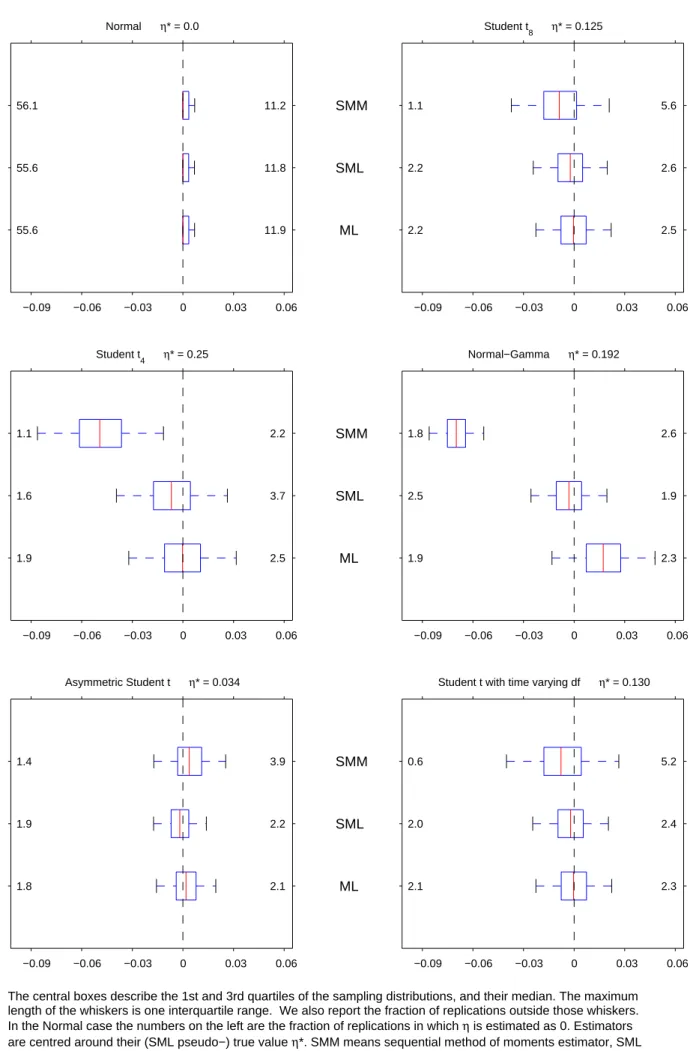
6.2 Sampling distributions of estimators
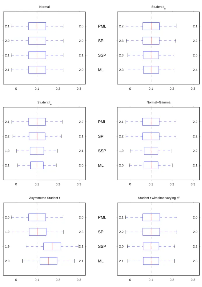
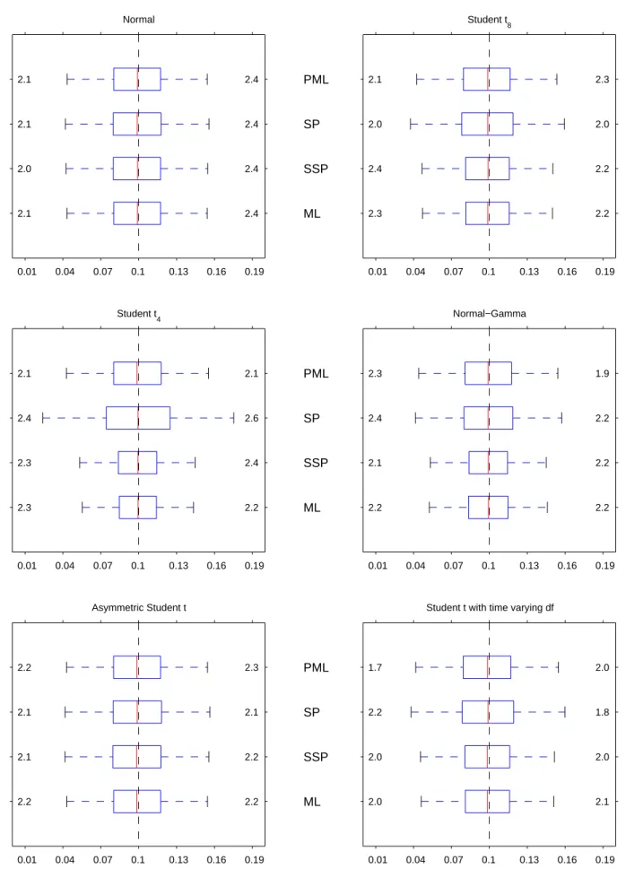
Figures 1A-1F display box-plots with the sampling distributions of the Gaussian- andt-based ML estimators, and the two semiparametric ones. In the case of vector parameters, we report the values corresponding to the third series. As usual, the central boxes describe the …rst and third quartiles of the sampling distributions, as well as their median. The maximum length of the whiskers is one interquartile range. Finally, we also report the fraction of estimates outside those whiskers to complement the information on the tails of the distributions.
As expected from Proposition 9.1, the distribution of the four estimators is essentially iden-tical under normality across all the parameters, with the only exception of the SP estimator of
3, which is not very surprising given that the ML and PML are numerically identical over half
the time. However, they progressively di¤er under correct studentt speci…cation as the degrees of freedom decrease.
Another thing to note is that the sampling distributions of the Gaussian PML estimators of 3 and 3 do not seem to be a¤ected much by the true conditional distribution of the data,
which suggests that the di¤erent information bounds of the simulated model are almost block diagonal between the conditional mean parameters ( ; ) and the rest. The same seems to be true for the SP estimator of 3, which is in line with Proposition 11, and essentially re‡ects the
fact that there is no SP adjustment for unconditional means. In contrast, the behaviour of the SP estimator of the autoregressive coe¢ cient 3 described in Figure 1B is very much at odds with the same proposition, probably as a result of the fact that the adjustment of this parameter described in (22) becomes very noisy once we replace the unknown score by the one obtained with the multivariate kernel estimator.
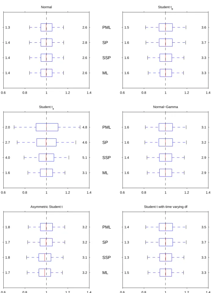
On the other hand, the sampling distributions of the SSP and t-based ML estimators of
3 and 3 are quite sensitive to the nature of the underlying distribution. In particular, when
the true distribution is elliptical, the sampling distributions of those estimators are narrower than the distributions of the PML and SP estimators. This is particularly noticeable in thet4
case, but also in the normal-gamma case, for which the ML estimator should lose its asymptotic 1 0
We considered .3, .5, .8, 1, 1.25, 1.5, 2, 2.5, 3 and 4 times the bandwidth[4=(N+ 2)]1=(N+4) s T 1=(N+4)
recommended by Silverman (1986) for multivariate density estimation under normality, where s2 is the second sample moment of "it(~T) averaged across tand iin the case of the SP estimator, and the sample variance of
3
q
e¢ ciency but not its consistency according to Proposition 16. At the same time, an asymmetric distribution introduces substantial positive biases in the ML and SSP estimators of 3.
Intu-itively, since the true distribution of the standardised innovations is negatively skewed, those estimators are re-centring their estimated distributions so as to make them more symmetric. Somewhat surprisingly, though, the biases in the unconditional mean seem to go a long way in mopping up the biases in the autocorrelation coe¢ cients. As for time-varying kurtosis, it seems to have little e¤ect on the estimators of the two conditional mean parameters that we analyse, with results that broadly resemble the ones obtained for thet8.
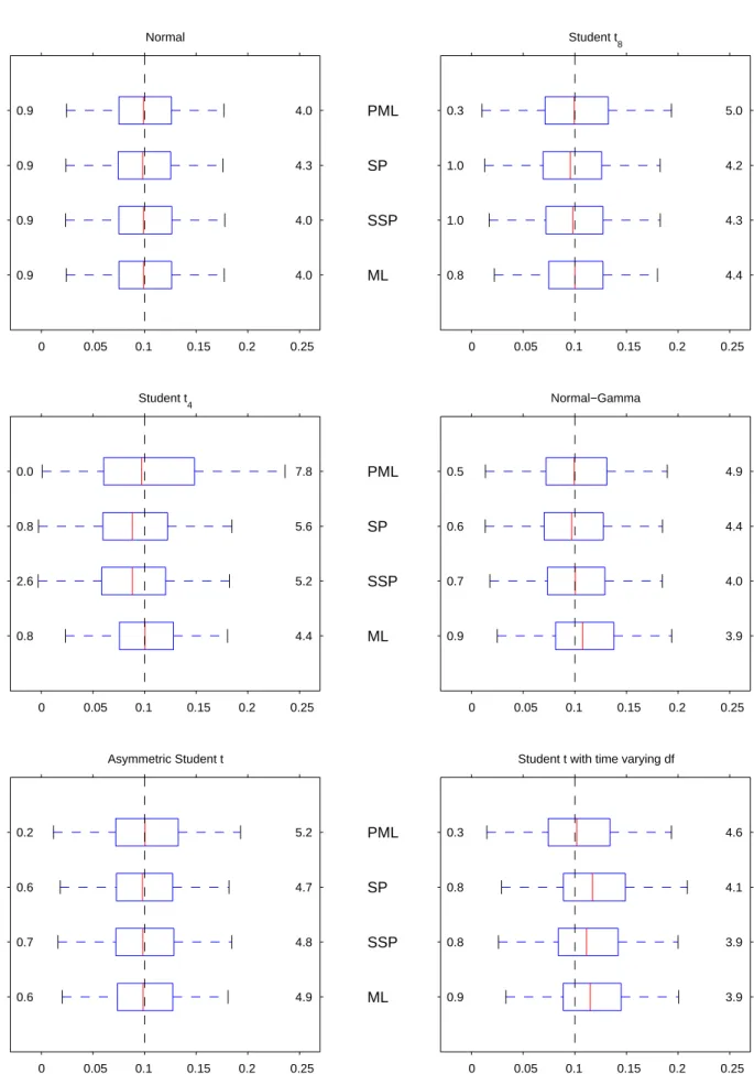
Unlike what happens with the conditional mean parameters, the sampling distributions of the PML estimators of both the static variance parametersc3 and 3, and the dynamic variance
parameters and are quite sensitive to the distribution of the innovations. In this sense, the …rst thing to note is that those sampling distributions deteriorate as the distribution of the standardised innovations becomes more leptokurtic. In fact, when 0 = 4 the shape of the
distribution of the PML estimators of theArchandGarchparameters is clearly non-standard, as discussed after Proposition 2. On the other hand, the PML estimators of and are the least a¤ected by the existence of time-varying higher order moments. The SP estimators of the conditional variance parameters also su¤er when 0increases, becoming substantially downward
biased in the case of 3, as well as in the case of when the innovations are t4.
In contrast, the ML estimators of the conditional variance parameters behave very much as expected: there are substantial e¢ ciency gains when the distribution of the innovations coincides with the assumed one, and some noticeable biases when it does not. However, it is interesting to note that those biases only a¤ect 3 and in the normal-gamma case, and and in the time-varying leptokurtic case. The unbiasedness results that we obtain with the asymmetric t
are somewhat remarkable, and suggest once again that the biases in the unconditional mean that we observe in Figure 1A adequately re-centre the estimated distribution of the innovations. The behaviour of the SSP estimators of the conditional variance parameters is mixed. When the distribution is elliptical, this estimator does a reasonably good job, although by no means does it achieve the e¢ ciency of the ML estimator. This is especially true in the case of t4
innovations, when it also shares a downward bias for with the SP estimator. Like the ML estimators, though, the SSP estimators also seem somewhat resilient to misspeci…cation, since the only noticeable biases correspond to 3 for the asymmetric studentt, and and for thet
distribution with time-varying degrees of freedom.
Model (27) can be easily reparametrised as in (28) if we ignore the sm