Predicting Diabetes Onset: an Ensemble Supervised
Learning Approach
Nonso Nnamoko Department of Computer Science Liverpool John Moores University Liverpool, L3 3AF, United Kingdom
Abir Hussain
Department of Computer Science Liverpool John Moores University Liverpool, L3 3AF, United Kingdom
David England
Department of Computer Science Liverpool John Moores University Liverpool, L3 3AF, United Kingdom
[email protected] Abstract—An exploratory research is presented to gauge the
impact of feature selection on heterogeneous ensembles. The task is to predict diabetes onset with healthcare data obtained from UC Irvine (UCI) database. Evidence suggests that accuracy and diversity are the two vital requirements to achieve good ensembles. Therefore, the research presented in this paper exploits diversity from heterogeneous base classifiers; and the optimisation effect of feature subset selection in order to improve accuracy. Five widely used classifiers are employed for the ensembles and a meta-classifier is used to aggregate their outputs. The results are presented and compared with similar studies that used the same dataset within the literature. It is shown that by using the proposed method, diabetes onset prediction can be done with higher accuracy.
Keywords—machine learning; ensembles; diabetes prediction; feature selection
I. INTRODUCTION
Diabetes is a global issue and recent estimates suggest that around 381.8 million adults aged 18 and over are living with diabetes [1]. The situation becomes even more complicated with 45.8% of adults estimated to have undiagnosed diabetes globally [2]. Without the appropriate models and resources (e.g., data) for early detection, people with diabetes may only be diagnosed after the onset of complications. However, with the advent of data collection technologies, healthcare data is becoming increasingly accessible. Machine learning can be used to construct computer models with capability to learn from such data so that predictions can be made on new examples without being explicitly programmed [3].
A single classifier can be trained to make predictions on unseen data. However, advances in machine learning have given rise to multiple classifier learning (also known as ensembles) [4], and this is widely known to perform better than single classifiers [5]. An ensemble is constructed by training a pool of single classifiers on a given training dataset and subsequently combining their outputs with a function for final prediction [6]. Thus, when an unseen data instance is presented, each classifier in the ensemble is asked for its prediction, and finally all predictions are combined using the combiner function.
There is consensus within the literature that accuracy and diversity are the two vital requirements to achieve good ensembles. Single classifiers such as neural network and C4.5 decision trees are often used to construct a variety of ensembles
due to their sensitivity to change(s) in the dataset. However, diversity (i.e., individual bias) in such situations are limited to data manipulation only [7]. Therefore, the method presented in this paper exploits diversity in the form of heterogeneous base classifiers, each trained with specific feature subset of the training data that leads to optimum accuracy. Five widely used classifiers are employed as base learners namely: Sequential Minimal Optimization (SMO), Radial Basis Function (RBF), C4.5 decision tree, Naïve Bayes (NB) and Repeated Incremental Pruning to Produce Error Reduction (RIPPER). It is expected that their individual biases would introduce diversity, and the classifier induced feature subsets would improve accuracy; ultimately leading to construction of good ensembles. All possible combinations of the five classifiers are explored, using both the full training dataset and feature selected subsets. A comparative study is conducted between the most accurate ensembles from both groups; to measure the impact of feature selection and its significance in improving ensemble accuracy. The results are also compared with similar studies that used the same dataset within the literature.
II. BACKGROUND
One of the most active areas of research in ensembles has been to study methods for constructing good pool of classifiers. Early ensemble methods, such as Bayesian model, evaluates the samples of each model individually and their predictions are averaged and weighted by how good they are [8]. Other general purpose ensemble methods exist, each focusing on one or more aspects of the ensemble learning process. For simplicity, only those involving data manipulation are discussed in this paper.
A common way to construct ensembles is by manipulating the input data fed to a single classifier. This can be achieved by running the classifier with a training set that consists of a sample drawn randomly with replacement from the original dataset. Such a training set is called a bootstrap replicate of the original training set and the technique is called Bagging (derived from bootstrap aggregation [9]).
A more advanced method for manipulating the training dataset is illustrated by the AdaBoost algorithm [10]. Like Bagging, AdaBoost manipulates the training examples to generate multiple models. However, AdaBoost maintains a set of weights over the training samples. In each run, a sample is used to train the classifier and the weighted error of the resultant model is computed. This weight is used to update the
weights on the other training samples by placing more weight on training samples that are misclassified; and less weight on those that are correctly classified.
Dietterich and Bakiri [11] described a technique for multi-class data called error-correcting output coding. In this method, the original classes are randomly partitioned into two subsets and the input data are re-classed based on the subset in which their original class belong. The re-classed data are used to constructs a classifier. By repeating this process, ensemble classifiers are obtained.
Another widely used technique for generating multiple classifiers is to manipulate the input data features. The process (commonly called feature selection [12]) is used to select a subset of the input data that contain useful features. A major disadvantage is that some features that may seem less important, and are thus discarded, may bear valuable information. This is where ensembles come into play by simply partitioning the input features among the individual classifiers in the ensemble. Hence, no information is discarded.
Initial implementations of feature selected ensembles used random or grouped features for training classifiers. Liao and Moody [13] group the input features into clusters based on their mutual information, such that features in each group are greatly correlated to each other, and less correlated with features in other groups. Tumer and Oza [14] presented a similar method in which the grouping is based on the class values. The features are grouped based on correlation with the class.
In an image analysis problem, Cherkauer [15] trained an ensemble of 32 neural networks by grouping together features that illustrate different image processing operations. Tumer and Ghosh [16] applied a similar technique to a sonar dataset by grouping features with similar characteristics and discarded those that did not fit into any group. Other researchers implemented the grouping strategy with random selection so that none of the input features are discarded [17]–[19].
The methods discussed so far share some similarities in that they assign features to each individual classifier model randomly or through some form of grouping. However, further strategies have been developed that uses more advanced selection process. Among them, Günter and Bunke [20] who proposed an ensemble method based on two feature selection algorithms, namely floating sequential forward and backward search algorithms [21]. In this approach, each classifier is given a well performing set of features using any of the two feature selection algorithms. The approach is similar to the one adopted in this paper, except that the classifiers are not heterogeneous.
III. EXPERIMENTAL DESIGN
A. Data
The data was obtained from UCI Machine Learning Repository [22], and originates from a national study conducted on the Pima Indian population [23]. The study is a standardised health check conducted every two years, in which community residents are tested for diabetes. However, only a fraction of the original data consisting of female subjects aged
21 or above was made available in UC Irvine database. The data consists of 768 samples, each defined as a row vector with eight features and a class value (i.e., negative or positive). The class value is determined by selecting one examination per subject that revealed a negative test result for diabetes and met one of the following two criteria:
i. Diabetes is diagnosed within five years of the examination
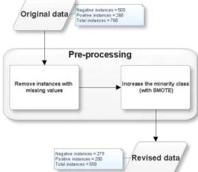
ii. Diagnosis test performed five years later is negative Of the samples, 500 tested negative and the rest (n = 268) tested positive over the 5 year period. Some abnormalities are evident in the data. For instance, some data instances have blood pressure value of zero. Such abnormality in the dataset could be due to missing values or human error which is common in real life examples. The class categories are not equally represented in the data (i.e., 500 negative & 268 positive instances). To address these issues, two pre-processing operations are applied as shown in Figure 1.
Figure 1 Data pre-processing operations applied on the original dataset By removing instances with “0” values, the total data sample was reduced to 419 of which 279 tested negative and 140 tested positive. To ensure unbiased estimates of prediction during experiment, we used Synthetic Minority Over-sampling Technique (SMOTE) algorithm by Chawla et al. [24], to oversample the minority class. As a result, a better balance of 279 negative and 280 positive instances is obtained. The feature characteristics of the revised dataset are shown in Table I and we assumed that instances with ‘0’ value in the first feature indicated that the subject has never been pregnant. It is important to note that all reference to ‘full data’ in this paper refer to the revised dataset after pre-processing which contains 559 data instances.
B. Experiment
To construct the ensembles proposed in this paper, five classifiers are employed as base learners as illustrated in Table II, namely – SMO, RBF, C4.5, NB and RIPPER. The classifiers are purposefully selected, to represent the five broad families of machine learning algorithms. The idea is to overcome the limited diversity issue that may exist when using variations of a single classifier.
Table IIFive broad machine learning approaches and associated algorithms
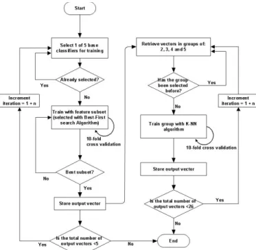
In a nut shell, all the five base classifiers are used to induce the features within the experimental data that leads to optimum accuracy. The feature search is conducted with best-first search algorithm [25]. The algorithm is known to be very greedy because it prefers states that look good very early in the search. To ensure that a thorough search was conducted, bi-directional approach was used. In the forward search, the algorithm starts with a preferred feature and incrementally adds other features. At each increment, the new subset is evaluated with an underlying classifier. The added feature is only kept if there is an increase in accuracy. The forward search also include a back tracking operation in which features added earlier are eliminated to check if this leads to improved accuracy. This dynamic continues until the desired subset is reached. The procedure is the same for backward search except that it begins with all the features and eliminates them until a desired subset (same as in forward search) is reached. 10-fold cross-validation is used during classifier training. Figure 2 shows a high level diagram of the proposed method.
Figure 2 High level diagram of the proposed ensemble method
To construct the ensemble, stacked generalization strategy (commonly known as stacking) was employed which involves training the predictions of two or more classifiers on a given dataset, with an independent or meta-classifier [26]. Weighted K-nearest neighbour (k-NN) algorithm [27] is used as the meta-classifier. In this experiment, each neighbour is assigned a weight 1 , where is the distance to the neighbour. This is mainly due to issues of class overlapping and imbalance observed in the training dataset. Although SMOTE is used to obtain a near balanced dataset, visualisation of the data points shows that the classes are not linearly separable. A 2D scatterplot of body mass index (BMI) and other features of the dataset is shown in Figure 3 (blue dots = positive & red dots = negative).
Figure 3 Data cluster of BMI and other features of the training dataset In total, two groups of 26 ensemble models are trained by exploiting outputs from the five base classifiers in all the possible combinations (using full dataset and feature selected subset). The results are used to conduct a comparative analyses presented in section V.
IV. RESULTS
The results are analysed with a modular approach so that individual components of the method are discussed appropriately. Four performance evaluation metrics are considered, including Accuracy, Sensitivity, Specificity and Area under the Receiver Operative Curve (AUC). These are all derived from a contingency table [28]. In this case, the Accuracy measures the total number of correct predictions. Sensitivity only measures the proportion of positive instances that are correctly identified while specificity measures the proportion of negatives that are correctly identified as such.
Comparative evaluation is also performed with McNemar’s test, to measure the accuracy difference between the proposed model and (i) the most accurate base learner and (ii) the most accurate ensemble; when trained on full dataset. Mc Nemar’s test [29] is a non-parametric test on a 2x2 classification table to measure the difference between paired proportions as illustrated in Table III.
Table III Possible results of two classifier algorithms
denotes the number of times both classifiers failed to classify instances correctly and denotes success for both classifiers. These two values do not give much information
about the classifiers’ performances as they do not indicate how their performances differ. However, the other two parameters ( ), show cases where one of the classifier failed and the other succeeded; indicating the performance discrepancies.
Table IV shows the base level results when trained on full dataset. From the table, it appears that the RIPPER and RBF models are the most accurate (78%). Accuracy assumes even class balance with equal error cost but this is not always the case in real world examples and certainly not in the research reported in this paper where the abnormal class is disproportionately lower; and the cost of misclassifying an abnormal example as normal is much higher. Consider the binary classification of the UK population as either positive or negative in terms of diabetes. Recent estimates suggest that 4.6% of the population are affected [30], leaving 95.4% normal cases. A model that predicts all the normal class correctly and all the minority class wrong would give a very high but misleading accuracy of 95.4%. Therefore, to determine the superior model between RBF and RIPPER models, there is a need to look at the parameters from which the accuracy value was calculated.
Table IV Result of base learners trained with full dataset
Compared to RBF, the RIPPER model predicted more instances correctly ( + = 437). However, predictions of the minority class are proportionately lower with the RIPPER model ( = 223) compared to RBF model (TP = 229). The nature of the model discussed in this chapter requires a fairly high rate of correct detection in the minority class (i.e., TP or positive diagnoses). Given that RBF model produced relatively higher true positives ( = 229) and thus lower false positives ( = 51), it is fair to say that RBF is slightly more accurate than RIPPER when trained on full dataset.
Table V shows the feature selected subset for each classifier, as well as the results obtained. Outputs from the base classifiers (trained on full dataset and feature selected subset) are used in all possible combinations to train ensemble models using KNN algorithm. The results are shown in Table VI.
Table VResult of base learners trained with feature selected subset
As shown in Table V, RBF is more accurate than the other base classifiers when trained on feature selected subset. However, its true positive result is higher when trained with full data ( = 229) than with feature selected subset ( = 226). Based on this, it was decided to use RBF result on full data as a benchmark against which the proposed ensemble method is measured, to determine if improvement is made.
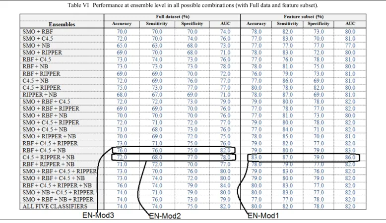
Table VI shows the results from both ensemble groups. (trained on the best feature subset). In total, 52 ensemble models are trained (i.e., 26 with full dataset and 26 with feature selected subset). The aim is to compare the results of the best ensemble from both groups. Of those trained with feature selected subset, the combination of C4.5 + RIPPER + NB clearly performed better than the rest on all the metrics, thus selected as the preferred ensemble model from the group. Henceforth, this model would be called ‘EN-mod1’ for simplicity. The same combination (trained with full data) would be referred to as ‘EN-mod2’. However, EN-Mod2 is not the best among the ensemble models trained with full dataset. In this group, the combination of RBF + C4.5 + NB is the best, and thus selected as the preferred ensemble model from this group. Henceforth, this model would be called ‘EN-mod3’ for simplicity. Result from these models are compared and analysed in the next section.
V. ANALYSIS
This section presents a comparative analysis between the models identified in section IV, in order to show the superiority of the ensemble method implemented.
A. RBF Vs EN-Mod1
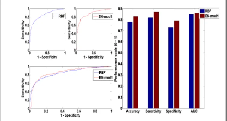
As shown in Figure 4, EN-mod1 clearly improved the results obtained with RBF model, by 5% in accuracy, sensitivity and specificity. The AUC was improved by 1%. To examine the significance of this improvement, Mc Nemar’s test was conducted (see Figure 5).
Figure 4 Graphic representation of EN-mod1 vs RBF model performance
EN-mod1 classified 83.0% of the instances correctly while RBF correctly classified 77.6%. The accuracy difference between both models is 5.37% which is significant at 95% confidence interval (P=0.0332)
Figure 5 EN-mod1 vs RBF performance showing Accuracy, Sensitivity, Specificity, AUC and Mc Nemar’s test
B. EN-Mod1Vs (EN-Mod2 & EN-Mod3)
As it can be seen from Table VI, EN-Mod1 performed better than its counterpart trained on full dataset (i.e., EN-mod2). However, EN-Mod2 is not the best ensemble within this group. Therefore, it is important to compare EN-Mod1 performance with the best ensemble trained with full dataset (i.e., EN-Mod3). As shown in Figure 6, EN-mod1 performed considerably better than EN-mod3 in all the metrics.
Figure 6 EN-mod1 vs EN-mod3 performance using Accuracy, Sensitivity, Specificity, AUC and Mc Nemar’s test
The accuracy difference between the two models is 7.33%
in favour of EN-mod1, at 95% confidence interval from 2.63%
to 12.04%, which is significant (P=0.0030). This affirms the significance of feature selection in the ensemble method reported in this paper. Considerable difference in AUC performance (4%) is also recorded in favour of EN-mod1 as shown in Figure 7. Therefore, it can be said that the ensemble method implemented in this paper is fit for purpose.
Figure 7 Graphic representation of EN-mod1 vs EN-mod3 model performance on AUC.
C. RBF vs (EN-Mod2 & EN-Mod3)
In the comparative study between RBF and EN-Mod1, it can be noted that significant improvement was made at ensemble level when trained with feature selected subset of the experimental data. To fully understand the effects of redundant features, there is need to compare RBF performance with ensembles trained with full dataset (i.e., EN-Mod2 and EN-Mod3).
As shown in Figure 8, RBF performed better than EN-Mod2. Accuracy is better with RBF (78%) in comparison to EN-mod2 (72%). The difference is 5.55%, which is significant at 95% confidence interval (P=0.0433).
Figure 8 : EN-mod2 vs RBF performance showing Accuracy, Sensitivity, Specificity, AUC and Mc Nemar’s test
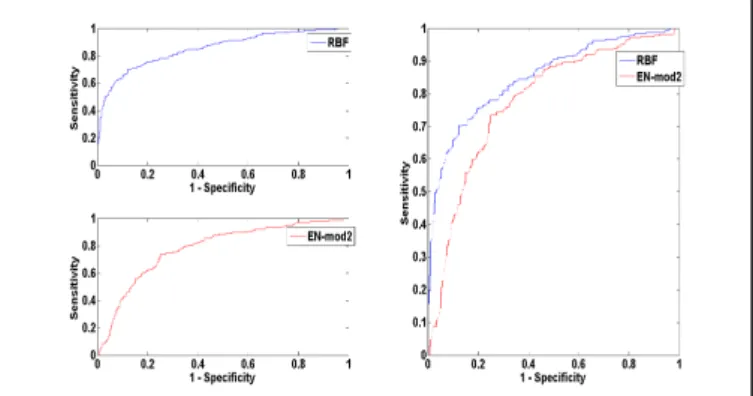
RBF also improved sensitivity by (14%) and specificity by (-4%). Negative difference is preferred for specificity due to the nature of classification problem. Visual representation of the AUC results is shown in Figure 9, in which RBF performed better by 7%.
Figure 9 : Graphic representation of EN-mod2 vs RBF model performance on AUC
RBF comparison with EN-Mod3 shows similar results (see Table VI). The results highlight the negative impact of redundant features on classification tasks, particularly in complex data situations. This was overcome through feature selection at base level, ultimately leading to improved performance obtained with EN-Mod1.
VI. CONCLUSION
Based on the results, ensemble models tend to yield better results than individual constituent classifiers. However this is not a certainty, as various factors may affect their ability to improve on performance, particularly at base level training.
Issues such as redundant features, class imbalance and skewed class distribution within the training data were found to be major contributors to low performance. For instance, penalty that occurs if redundant features and overlapping class is not properly accounted for is evident in Table VI (see also Figure 3 for class coupling issues). The results show that the penalty on accuracy can be quite significant. Nonetheless, the correction strategy implemented suggests that feature selection applied at base level training has the potential to produce lower ensemble error.
Further observations from the experiment suggest that the highly desirable diversity when training ensembles can be achieved by using base classifiers un-related to each other. Much of the previous work on ensemble classifier models have focused on a collection of a single base classifier trained in several variations. In this research, the base classifiers are selected from five broad families of machine learning algorithms. Therefore, each classifier would induce models based on its operational characteristics. Although none of them made improvement(s) of any significance at base level, the cumulative of their individual biases contributed to wider knowledge at ensemble level about the classification problem being addressed; ultimately leading to significant improvement.
It is worth mentioning that the vast majority of reported experiments in diabetes prediction only enhanced classification accuracy up to 82% [185]. In fact, literature search of all the research conducted with the same dataset revealed a total of 70 eligible studies with accuracy results ranging from 59.5% to 82% (see Table VII). Our research produced 83%, so the implemented method can be said to perform relatively well. It is important to note that the research studies shown in Table VII may have used the Pima diabetes dataset in its original form (i.e., without eliminating the impossible values and/or applying SMOTE). As such, their results may be different if such pre-processing experiments were conducted. That said, results from our research indicate that improvements were made as a result of feature selection applied to heterogeneous base learners; and not necessarily data pre-processing. For instance, Figure 3 indicates that the pre-processing exercise did not make much difference to class reparability which is the major issue with the Pima diabetes dataset. In fact, one of the studies listed in Table VII trained an RBF model with the original dataset and the accuracy result is 68.23%.
REFERENCES
[1] L. Guariguata, D. R. Whiting, I. Hambleton, J. Beagley, U. Linnenkamp, and J. E. Shaw, “Global estimates of diabetes prevalence for 2013 and projections for 2035,” Diabetes Res. Clin. Pract., vol. 103, no. 2, pp. 137–149, Feb. 2014.
[2] J. Beagley, L. Guariguata, C. Weil, and A. A. Motala, “Global estimates of undiagnosed diabetes in adults,” Diabetes Res. Clin. Pract., vol. 103, no. 2, pp. 150–160, Feb. 2014.
[3] A. Munoz, “Machine Learning and Optimization,” 2014. [Online]. Available: https://www.cims.nyu.edu/~munoz/files/ml_optimization.pdf. [Accessed: 29-Jul-2017].
[4] L. K. Hansen and P. Salamon, “Neural Network Ensembles,” IEEE Trans. Pattern Anal. Mach. Intell., vol. 12, no. October, pp. 993–1001, 1990.
[5] L. I. Kuncheva, Combining pattern classifiers: methods and algorithms, 2nd ed. Wiley, 2014.
[6] N. Nnamoko, F. Arshad, D. England, and J. Vora, “Meta-classification Model for Diabetes onset forecast: a proof of concept,” in IEEE International Conference on Bioinformatics and Biomedicine Workshops, 2014, pp. 50–56.
[7] T. G. Dietterich, “Multiple Classifier Systems,” in Lecture Notes in Computer Science, vol. 1857, Berlin, Heidelberg: Springer Berlin Heidelberg, 2000, pp. 1–15.
[8] T. M. Fragoso and F. L. Neto, “Bayesian model averaging: A systematic review and conceptual classification,” arXiv preprin, vol. 1509.08864, 2015.
[9] L. Breiman, “Bagging predictors,” Mach. Learn., vol. 24, no. 2, pp. 123– 140, Aug. 1996.
[10] Y. Freund and R. E. Schapire, “A Decision-Theoretic Generalization of On-Line Learning and an Application to Boosting,” J. Comput. Syst. Sci., vol. 55, no. 1, pp. 119–139, Aug. 1997.
[11] T. G. Dietterich and G. Bakiri, “Solving Multiclass Learning Problems via Error-Correcting Output Codes,” Artif. Intell. Res., vol. 2, pp. 263– 286, 1995.
[12] N. Nnamoko, F. Arshad, D. England, J. Vora, and J. Norman, “Evaluation of Filter and Wrapper Methods for Feature Selection in Supervised Machine Learning,” in PGNET, 2014, pp. 63–67.
[13] Y. Liao and J. E. Moody, “Constructing Heterogeneous Committees Using Input Feature Grouping: Application to Economic Forecasting,” Adv. Neural Inf. Process. Syst., vol. 12, pp. 921–927, 2000.
[14] N. C. Oza and K. Tumer, “Input Decimation Ensembles: Decorrelation through Dimensionality Reduction,” in Multiple Classifier Systems, 2001, pp. 238–247.
[15] K. J. Cherkauer, “Human Expert-Level Performance on a Scientific Image Analysis Task by a System Using Combined Artificial Neural Networks,” in Integrating Multiple Learned Models for Improving and Scaling Machine Learning Algorithms Wkshp, 13th Nat Conf on Artificial Intelligence, 1996, pp. 15–21.
[16] K. Tumer and J. Ghosh, “Error Correlation and Error Reduction in Ensemble Classifiers,” Conn. Sci., vol. 8, no. 3–4, pp. 385–404, Dec. 1996.
[17] Tin Kam Ho, “Random Decision Forests,” in Proceedings of 3rd International Conference on Document Analysis and Recognition, 1995, vol. 1, pp. 278–282.
[18] T. K. Ho, “The Random Subspace Method for Cosntructing Decision Forests,” IEEE Trans. Pat- tern Anal. Mach. Intell., vol. 20, no. 8, pp. 832–844, 1998.
[19] S. D. Bay, “Combining Nearest Neighbor Classifiers Through Multiple Feature Subsets,” in Proceedings of the 17th International Conference on Machine Learning, 1998, pp. 37–45.
[20] S. Gunter and H. Bunke, “Creation of classifier ensembles for handwritten word recognition using feature selection algorithms,” in Proceedings Eighth International Workshop on Frontiers in Handwriting Recognition, 2002, pp. 183–188.
[21] P. Pudil, F. J. Ferri, J. Novovicova, and J. Kittler, “Floating Search Methods for Feature Selection with Nonmonotonic Criterion Functions,” in Proceedings of the 12th IAPR International Conference on Pattern Recognition (Cat. No.94CH3440-5), 1994, vol. 2, pp. 279–283. [22] M. Lichman, “UCI Machine Learning Repository.” Irvine, CA:
University of California, School of Information and Computer Science, 2013.
[23] J. W. Smith, J. E. Everhart, W. C. Dicksont, W. C. Knowler, and R. S. Johannes, “Using the ADAP Learning Algorithm to Forecast the Onset of Diabetes Mellitus,” in Proc Annu Symp Comput Appl Med Care, 1988, pp. 261–265.
[24] N. V Chawla, K. W. Bowyer, L. O. Hall, and W. P. Kegelmeyer, “SMOTE : Synthetic Minority Over-sampling Technique,” J. Artificial Intell. Res., vol. 16, pp. 321–357, 2002.
[25] R. Dechter and J. Pearl, “Generalized best-first search strategies and the optimality af A*,” J. ACM, vol. 32, no. 3, pp. 505–536, Jul. 1985. [26] D. C. Klonoff, B. Buckingham, J. S. Christiansen, V. M. Montori, W. V
Tamborlane, R. a Vigersky, and H. Wolpert, “Continuous glucose monitoring: an Endocrine Society Clinical Practice Guideline.,” J. Clin. Endocrinol. Metab., vol. 96, no. 10, pp. 2968–79, Oct. 2011.
[27] K. Hechenbichler and K. Schliep, “Weighted k-Nearest-Neighbor Techniques and Ordinal Classification,” Sonderforschungsbereich, vol. 386, 2004.
[28] G. Canbek, S. Sagiroglu, T. T. Temizel, and N. Baykal, “Binary classification performance measures/metrics: A comprehensive visualized roadmap to gain new insights,” in 2017 International Conference on Computer Science and Engineering (UBMK), 2017, pp. 821–826. [29] Q. McNemar, “Note on the sampling error of the difference between
correlated proportions or percentages,” Psychometrika, vol. 12, no. 2, pp. 153–157, Jun. 1947.
[30] Diabetes UK, “Diabetes : Facts and Stats,” 2014. [Online]. Available: https://www.diabetes.org.uk/resources-s3/2017-11/diabetes-key-stats-guidelines-april2014.pdf. [Accessed: 25-Jan-2018].