Automatic Composition of Music with Methods of Computational Intelligence

Automatic Composition of Music with

Methods of Computational Intelligence

ROMAN KLINGER Fraunhofer Institute for

Algorithms and Scientific Computation Department of Bioinformatics Schloss Birlinghoven, 53754 Sankt Augustin

GERMANY [email protected]

GÜNTER RUDOLPH University of Dortmund Department of Computer Science LS XI – Computational Intelligence

44221 Dortmund GERMANY

[email protected]

Abstract:We describe our approach for the automatic composition of monophone melodies on a user given chord sequence. For this purpose we use Markov-chains and other methods to build some initial individuals. These are then optimised with evolutionary algorithms using automatically learned classifiers next to interactive evaluation as fitness functions.

Key–Words:computational Intelligence, automatic composition, music, decision tree, neural network, evolutionary algorithm, Markov-chains, Markov-models

1 Introduction

The main motivation for developing a program for au-tomatic composition is to attach importance on get-ting melodies that have something new: The pro-gram should simulate creativity so that it can be used for composition assistence. Similar to the work of Biles [2, 3] or Wiggins and Papadopoulos [14] we use an evolutionary algorithm. Biles uses an interac-tive method as evaluation function, Wiggins and Pa-padopoulos use weighted sums of numerical features values extracted from the melodies. The interactive approach has the disadvantage of requiring much time to evaluate melodies. Using weighted sums raises the question if that method maps the personal taste of mu-sic appropriately.

There have been some approaches to learn a fit-ness function, for example with neural networks, but without emphasizing creativity [5], so the generated melodies are not pleasing to the ear [4] or they are just not very interesting [10].

Our idea is to extract features [19, 21] on which a data mining algorithm can classify the melodies. That approach has the advantage of the possibility that the automatically generated classifier fits the user’s taste and can classify the melodies fast.

Next to the evaluation function another important

∗

This is an extended version of [12].

element of the evolutionary algorithm is the initial-isation for which we not only use purely randomly assigned note lengths and pitches but more complex methods like Markov chains of different order. A great introduction to the modelling of interrelations in mu-sic with statistical methods can be found in [23].

Another important thing to point out is that the implementation is licensed under the Gnu Public Li-cence1 so that everyone can try out the program and experiment with different parameters2. This is a spe-cial feature because most systems for automatic com-position are closed source apparently.

The rest of the paper is organised as follows: At first we explain the evolutionary algorithm developed here before we look at the methods for building the initial population. Then some of the variation opera-tors are described and elucidated on some examples. The probably most important part of our work is the evaluation procedure for melodies which will be ex-plained next. The last section is a conclusion and an outlook on future work.

1

http://www.gnu.org/copyleft/gpl.html

2

Download information can be found on

http://www.romanklinger.de/musicomp/musicomp.html and on

2 Overview

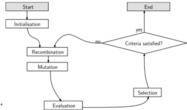
An evolutionary algorithm [1] is an optimization scheme which works on a set on possible solutions, in our case on melodies. A visualisation is given in figure 1. ‘ ‘ Start Criteria satisfied? End Recombination Mutation Initialisation Evaluation Selection no yes

Fig. 1: Main components of an evolutionary algo-rithm.

At first the set of solutions, also called population of individuals, is initialised. This is done by using statistical methods like Markov chains so that they are meaningful according to some musical laws. For that, the user specifies the chords on which the melody should be played. After that this set is altered by mu-tation and recombination of the individuals. Then the original individuals and the altered ones are evaluated by some fitness function. The best ones, in our case the hopefully most pleasant melodies, form the subse-quent population.

3 Initialisation

For using the optimisation scheme of evolutionary al-gorithms it is necessary to build an initial population of melodies. We use different methods, distinguishing between those for developing the rhythm and those for fixing the pitches of the notes. The general workflow for the initialisation is as follows:

Define Rhythm ⇓ Set Pitches

⇓ Postprocess

Implemented methods for defining the rhythm are Markov chains [9], Pattern sets and random assign-ment using a uniform distribution. Techniques for fix-ing the pitches are Markov chains, random walks and random assignment using a Gaussian distribution. The postprocessing adjusts possible inaccuracies relating to matching the note pitches to the given chord se-quence.

There are approaches using these methods inde-pendent to an optimisation scheme for generation of melodies (see [13, 20] for an overview) what has other needs than an initialisation for optimisation: Using them as a stand-alone method needs them to be more robust and providing nice melodies out of the box. In our case we want them to supply some creative and new aspects. For that they have to be parameterisable to find a trade-off between generating new melodies that are perhaps not pleasing before starting the evo-lutionary algorithm but having potentials in them and having good enough individuals for giving the optimi-sation a chance.

The simplest methods are the random assignments of lengths and pitches. For the rhythm, the parameters to set are the shortest and longest length. In this inter-vall a note with indexiat positionpiwith lengthliis

generated which starts at position pi−1+li−1. In

ad-dition, a propability is given that a “note” has no pitch but is a rest.

The pitches of the notes are set using the keynote of the given chord at the same timepoint with some Gaussian noise according to a standard deviation that must be specified as a parameter by the user.

Another simple method for generating the rhythm is the use of patterns. For that, the system reads some user given MIDI files from which only the rhythm is extracted in a user given length from the beginning. These patterns (one from each file) are then selected randomly and concatenated to get the rhythm for a new individual.

The most interesting and flexible idea to generate initial individuals is the use of Markov chains. For the melody the random walk is just a special case of that method. The Markov chains and their corresponding characteristic matrices are computed from a given set of MIDI files using a maximum-likelihood algorithm. As a representation for the Markov chains for generat-ing the rhythm we use integer valuesr. Ifr <0holds, it represents a rest, otherwise it describes a ’real’ note. The absolute value gives the length of the rest or the note where |r| = 1 is a quarter, |r| = 1₂ is an half-quarter and so on. An example of a first order Markov chain can be seen in figure 3.

G

4

4

ˇ ˇ ˇ ˇ ˇ ˇ ˇ ˇ ˘ ˇ ˇ ¯

Fig. 2: Example melody for generating Markov chains.

We always assume a melody to start with a tone af-ter the longest possible rest (represented by −4, real rests at the beginning of the melody are ignored). In

-4.0 1.0 1.0 0.8 2.0 0.1 4.0 0.1 1.0

Fig. 3: Example Markov chain generated from the melody in figure 2.

the example, always a quarter follows this virtual rest. With10%each a double-quarter or a whole note fol-lows. With 80% a quarter is followed by a quarter. The question arrises what happens after a whole note: In cases like that where no successive state is defined we start again like at the beginning of the rhythm.

For setting the pitches we have two possible vari-ants of the Markov chains. The one we callabsolute Markov chainworks on sequences of absolute pitch values, the one calledrelative Markov chainworks on sequences of intervalls between two successive notes. Examples can be found in figure 6(a) and 6(b). In the case of reaching a state without successor we choose the following pitch respectively intervall from the set of states with successors.

The main difference between the two different kinds of Markov chains is that absolute Markov chains are often more simple but the input MIDI files should be transposed to the goal scale and key. The relative Markov chains are not that dependent to the scale.

G

<

> ˇ ˇ` (ˇ ˇ

ˇ

ˇ`

(ˇ ˇ ˇ

ˇ ? (ˇ ˇ

ˇ

G

˘

>

ˇ

ˇ`

?

ˇ ˇ ˇ`

(ˇ ˇ ˇ

ˇ`

(ˇ ˇ ˇ ˘

<

chain (Auld Lang Syne)

Another important parameter of the Markov chains should be mentioned: It is possible to specify the order of the chain. This is useful to decide how similar the generated melodies should be to the input melodies from which the matrices are computed. Because of that in a Markov chain of order4we recognize whole bars of the input melodies. As an example in figure 5 generated rhythms using Markov chains of different order which are estimated fromAuld Lang Syne(figure 4) are displayed. We can see that they are more similar to the rhythm ofAuld Lang Synethe higher the order of the Markov chain is.

G4 4 ˇ ˘ > ˇ ˇ ? ˇ (ˇ8 (ˇ ˘ > (ˇ8 (ˇ ˇ ˇ` ˇ ˇ G4 4 ˇ ˇ ˇ ˇ ˇ` (ˇ ˇ ˇ ˇ` (ˇ ˇ ˇ ? (ˇ ˇ ˇ ˇ G4 4 ˇ ˘ > ˇ ˇ` (ˇ ˇ ˇ` (ˇ ˇ ˇ ˇ` (ˇ ˇ ˇ (a) 1st order G4 4 ˇ ˇ` (ˇ ˇ ˇ ˇ` (ˇ ˇ ˇ ˇ ˇ` (ˇ ˇ ˇ ˇ` (ˇ G4 4 ˇ ˇ` (ˇ ˇ ˇ ? (ˇ ˇ ˇ ˇ` (ˇ ˇ ˇ ? (ˇ ˇ ˇ ˇ G4 4 ˇ ˇ` (ˇ ˇ ˇ ˘ > ˇ ˇ` (ˇ ˇ ˇ ? (ˇ ˇ ˇ (b) 2nd order G4 4 ˇ ˇ` (ˇ ˇ ˇ ˇ ? (ˇ ˇ ˇ ˘ > ˇ ˇ` ˇ (ˇ G4 4 ˇ ˇ` (ˇ ˇ ˇ ˇ ? (ˇ ˇ ˇ ˇ ? (ˇ ˇ ˇ ˇ` (ˇ ˇ G4 4 ˇ ˇ` (ˇ ˇ ˇ ˇ ? (ˇ ˇ ˇ ˇ` (ˇ ˇ ˇ ˇ` (ˇ ˇ (c) 3rd order G4 4 ˇ ˇ` (ˇ ˇ ˇ ˇ ? (ˇ ˇ ˇ ˘ > ˇ ˇ` ˇ (ˇ G4 4 ˇ ˇ` (ˇ ˇ ˇ ˇ` (ˇ ˇ ˇ ˘ > ˇ ˇ` ˇ (ˇ G4 4 ˇ ˇ` (ˇ ˇ ˇ ˇ ? (ˇ ˇ ˇ ˘ > ˇ ˇ` ˇ (ˇ (d) 4th order

Fig. 5: Examples for rhythms, which were generated using Markov chains of different order esti-mated from the melody in figure 4.

For the initialisation of melodies it is recommended to use more than one method with not too strict pa-rameters so that the first population is diverse enough for building innovative melodies. The implemented program selects randomly from a set of user specified methods which one should be used for an individual.

Remarkable is the trade-off between conservative and innovative initialisation as visualised in table 1.

Innovative Conservative

Markov chains

complex simple

low order high order

Pattern sets

many patterns few patterns short patterns long patterns

Table 1: Trade-off between innovative and converva-tive initialisation. A 0.25 B 0.75 0.5 0.25 C 0.25 1.0 _D 1.0 _F 1.0 _E

(a) Absolute Markov chain

-2 1.0 2 0.5 0.25 0 3 0.25 0.5 1 0.5 1.0 -1 1.0

(b) Relative Markov chain

Fig. 6: Markov chains for the generation of pitch se-quences estimated using the melody in figure 2.

4 Mutation and Recombination

The operators mutation and recombinationrepresent the methods to change the melodies so that they en-hance their interestingness. Here we only give some examples because a description of the whole set of operators would exceed the size of the paper awfully. More details can be found in [11].

The mutation operators can be distinguished in those which change pitches (one-point-mutation, transposition, inversion), those which change rhythm (moving, merging, splitting of notes) and those which make some structural modification of the melody (ro-tating, sorting, mirroring of some range).

G

4

4

ˇ ˇ

ÂÂ

ˇ ˇ ˇ Ćơ

Fig. 7: Example of some melody prior to variation. For the examples we assume figure 7 being the orig-inal melody. An example for the one-point-mutation could be the melody in figure 8 in which the second note is raised by one half step and the fifth tone is raised by one step. That method changes the pitch of every note with a low probability. The stepsize is determined by a bilateral geometric distribution [18].

G

4

4

ˇ 4ˇ

ÂÂ

ˇ ˇ ˇ ˇ

Fig. 8: One-point-mutation of melody in figure 7. An example for changing the rhythm is splitting ev-ery note with a low probability as we can see in fig-ure 9. Here the second and the third note are split into two notes, each of half of the length of its original. The pitch of the second note is changed analogous to one-point mutation.

G

4

4

ˇ ˇ ˇ ˇ \ˇ ˇ ˇ Ĺš

Fig. 9: Splitting some notes of melody in figure 7.

G

4

4

ˇ ˇ

ÂÂ

ˇ ˇ ˇ ¡

Fig. 10: Sorting of melody in figure 7.

An example for a structural modification is sorting the notes downwards with respect to their pitches as

we can see in figure 10. Here the whole melody is sorted. In our implementation only a randomly deter-mined part of the melody is changed.

The recombination combines two parents to one or more new individuals. We experimented with interme-diate methods which work by using the mean pitches of two notes on the same point in time of the two par-ents. Here the problem in using that kind of operator is that the melodies tend to a single tone repetition. So the better choice is using a one-point-crossover which builds two individuals by beginning with the first par-ent and ending with another and the other way round. The crossover point is determined randomly. An ex-ample is shown in figure 11.

Parents: G4 4 ˇ ˇ ˇ ˇ ˇ ˇ ˇ ˇ ˇ ˇ ˇ ˇ ˇ ˇ \ˇ ˇ \ˇ \ˇ ˇ ˇ ˇ ˇ ˇ \ ÊÊ ˇ ˇ ˇ ˇ ˇ ˇ ˇ ˇ ˇ G4 4 < ˇ ˇ ˘ ˇ ˇ 4˘ 4ˇ ˇ ¯ Offspring: G4 4 ˇ ˇ ˇ ˇ ˇ ˇ ˇ ˇ ˇ ˇ ˇ ˇ ˇÈÈˇ ˇ \˘ 4ˇ ˇ ¯ G4 4 < ˇ ˇ ˘ ˇ 4ˇ_ŤŤˇ \ˇ \ˇ ˇ ˇ ˇ ˇ ˇ \ ÊÊ ˇ ˇ ˇ ˇ ˇ ˇ ˇ ˇ ˇ

Fig. 11: Example for one-point-crossover.

5 Selection

The operator selection builds the subsequent popula-tion. We tried to use fitness proportional selection, but this reduces the diversity of the individuals. It is nice not to have too similar individuals in the set because then it is more likely to have variations that could pos-sibly fit the personal taste. Actually, it is crucial to maintain diversity in the population to provide suffi-cient potential for continuing evolution. Determinis-tic selection as used in evolution strategies works very fine, especially with niching methods to enhance the diversity.

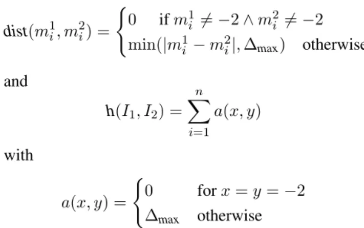
We use two niching methods [1]. The first,fitness sharing, works by scaling down the fitness of similar individuals. The second, in our case much more suc-cessful, is calledcrowding. Here two parents are re-combined to two children. The parents and children compete to each other in the pairing in which their similarity is higher. The function that gives the sim-ilarity between two individualsI1 andI2 with pitches

miat points of timeiis

sim(I1, I2) = 1−

Pn

i=1dist(m1i, m2i)

with dist(m1_i, m2_i) = ( 0 ifm1_i 6=−2∧m2_i 6=−2 min(|m1 i −m2i|,∆max) otherwise and h(I1, I2) = n X i=1 a(x, y) with a(x, y) = ( 0 forx=y=−2 ∆max otherwise

For understanding the formula above it is impor-tant to know about our representation of melodies: A melody is a tuplem ∈ {−2,−1,0, . . . ,127}n_where

i ∈ {1, . . . , n} are points of time and the values

0, . . . ,127 represent the start of a tone with a note pitch according to the general midi specification3. The value−1means “Holding the last event” and−2starts a rest.

We set ∆max = 4, which means that the largest

intervall between two pitches that is considered is4. This also holds for an interval between a “−1” and the starting of a note with a given pitch in two individuals at the same point of time.

That function emphasizes the importance of the rhythm, so especially rhythmic features of the melodies are kept over the generations.

6 Evaluation

The evaluation function is a very important point in the generation of melodies with evolutionary algorithms. It “restricts” the creativity of the mutation and recom-bination operators. In addition to the interactive eval-uation, which we also implemented in form of a slider the listener can move between 1 and 10 in steps of

0.01after the melody was played that has to be evalu-ated, we implemented some methods based on feature extractions.

6.1 Feature Extraction

The feature extraction follows the work presented in [19, 21] with some additional methods. The tures are subdivided into pitch features, tonale tures, contour features, rhythmic features, pattern tures, features for chord change and accentuation fea-tures. For explanation we give some examples which are all played on the chord sequence4: Am, Dm, E, Am

3

http://www.midi.org/about-midi/gm/gminfo.shtml 4

The chord Am is a set of the notes a, c, e. Dm is d, f, a. E is e, g#, b.

The featureHarmonicitygives the ratio between the number of notes with pitches of the current chord and the number of all notes. An example for two different melodies is given in figure 12.

G

4

˘ ˇ ˇ ˘ ˇ ˇ Z˘ ˇ ˇ ˘ ˘

G

4

˘ ˇ ˇ ˘ ˇ ˇ ˘ ˇ

ˇ ˘ ˘

Fig. 12: Example for featureHarmonicity. The value of the first melody is 0, the one for the second is 1.

G

4

˘ ˇ ˇ ˘ ˇ 2ˇ ˘ ˇ ˇ ¯

G

4

< ˇ ˇ < ˇ ˇ < ˇ 2ˇ ¯

Fig. 13: Example for featureRests on Downbeatswith a value of 0 in the first melody and a value of 0.75 in the second one.

G

4

ˇ ˇ ˇ ˇ ˇ ˇ \ˇ ^ˇ \ˇ \ˇ ˇ ˇ ˇ ˇ ˇ ˇ

G

4

ˇ ˇ ˇ ˇ ˇ ˇ ˇ ˇ ˇ ˇ ˇ ˇ ˇ ˇ ˇ ˇ

Fig. 14: Example for feature Repeated Pitch with a value of 0 in the first melody and a value of 1 in the second one.

The featureRests on Downbeatsdetermines the ra-tio between the number of downbeats and the number of downbeats on which there is a rest. In figure 13 are two melodies with 4 downbeats: One with a value of 0 with no rests and one with 3 rests and a resulting value of 0.75.

The featureRepeated Pitch computes the ratio be-tween the number of all intervalls with a size of0and the number of all intervals (=number of notes−1). In the example in figure 14 is one melody without pitch repetition (value 0) and one with all possible pitch rep-etitions (value 1).

6.2 Evaluation with Data Mining Methods Typical problems of interactive evaluation are the long time required for listening to the melodies, the subjec-tivity and that this methods are not always reliable. So a nice idea is to use machine learning on the features

mentioned before. We tried artificial neural networks and decision trees. For generating these we use a set of examples which were evaluated by a single person. It is composed of 45 well-known melodies with a major-ity of high evaluations, 136 automatically generated individuals (by saving all individuals of an evolution with interactive evaluation) and 24 outstanding unaes-thetic individuals with very low fitness values. The melodies are given in MIDI-Format with an XML-File specifying the chords and the fitness.

6.2.1 Using Feed Forward Neural Networks

It is possible to select the features that should be used as input for the neural net. For every feature we use one input neuron and in every net one output neuron which gives the evaluation.

We experimented with neural networks with differ-ent structures and detected that when using all 42 im-plemented features it is reasonable to use a fully con-nected net with one hidden layer of 35 neurons. We decided to use resilient propagation [17, 8] for training which lasts only few minutes. It is possible to reach a resubstitution error of0.022.

6.2.2 Using Decision Trees

Neural networks are theoretically capable of approxi-mating arbitrary functions, but the weights of the con-nections between the neurons are not intuitively inter-pretable. A very good approach for a better under-standable classifier are decision trees that are built up in an inductive way [15, 16]. The algorithm we use is called C4.5 and is implemented in the Weka-Library [22] for Java. This algorithm deals with continuous attributes which correspond to our features but cannot handle regression. Because of that the fitness values have to be discretized. So the user specifies a number of classes in which the fitness values of the individuals in the example set should be reclassified.

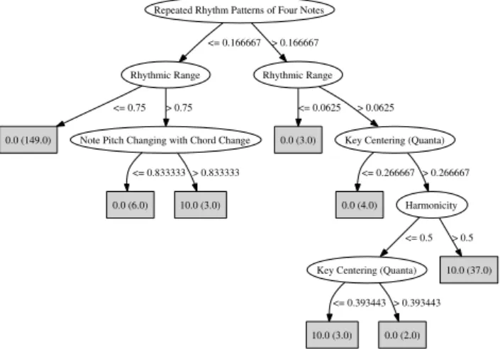
An example for an automatically generated decision tree using only 2 fitness classes (0and10) so that the tree is small enough to print it here is depicted in fig-ure 15 (the numbers in brackets give the number of classified examples on the according leave).

Already this small example provides the facility for interpretation. If the feature Repeated Rhythm Pat-terns of Four Notesis very small andRhythmic Range

is also not very high the individual is classified as a bad melody. But if theRhythmic Rangeis high and the

Note Pitch Changing with Chord Changeis also high it is classified as being a good one. Likely the follow-ing explanation holds: In the examples the chords are often changing with the bars. So if the rhythmic range

Repeated Rhythm Patterns of Four Notes

Rhythmic Range <= 0.166667 Rhythmic Range > 0.166667 0.0 (149.0) <= 0.75

Note Pitch Changing with Chord Change > 0.75 0.0 (6.0) <= 0.833333 10.0 (3.0) > 0.833333 0.0 (3.0) <= 0.0625

Key Centering (Quanta) > 0.0625

0.0 (4.0) <= 0.266667

Harmonicity > 0.266667

Key Centering (Quanta) <= 0.5 10.0 (37.0) > 0.5 10.0 (3.0) <= 0.393443 0.0 (2.0) > 0.393443

Fig. 15: Example for a decision tree for the classifica-tion of melodies. 0 2 4 6 8 10 12 14 l k j i h g f e d c b a

pruned decision tree, 5 fitness classes unpruned decision tree, 5 fitness classes decision tree, 11 fitness classes interactive

Fig. 16: Comparison of decision tree classifiers with interactive evaluation. 0 2 4 6 8 10 l k j i h g f e d c b a

neural net, 6 hidden neurons neural net, 35 hidden neurons interactive

Fig. 17: Comparison of neural net classifiers with in-teractive evaluation.

is high there is a good possibility that the rhythm is confusing, but if there is always a note on the first beat in a bar it is considered not bad.

7 Conclusions

Since it is difficult to evaluate the quality of the au-tomatic classification functions we used 10 different melodies and compared their automated classification with an interactive one. In figure 16 we see the

0 20 40 60 80 100 120 0 20 40 60 80 100 0.03 0.032 0.034 0.036 0.038 0.04 0.042 0.044 0.046 0.048 0.05 Number of Nodes Error Number of Classes

Tree Size (Pruned) Tree Size (Unpruned) Error (Pruned) Error (Unpruned)

Fig. 18: 10-fold crossvalidation of decision trees with different number of classes

parison of some decision trees. The classification of the one with 11 fitness classes is identical using a pruned and an unpruned variant so there is no differ-ence. The individualsa to l are sorted with respect to the interactive evaluation. The tree with 11 fitness classes makes some errors on the bad individuals and the unpruned one with 5 fitness classes is questionable in the middle fitness area. The pruned tree with 5 fit-ness classes leaves the best impression.

The comparison of the neural networks in figure 17 reveals that they are not very good in our configura-tion. Because of the very low TSSE and a small mean squared error using 10-fold-crossvalidation of0.025it is likely that there is a problem with overfitting (see section 6.2.1).

An evaluation using 10-fold-crossvalidation on the decision trees with different numbers of classes is displayed in figure 18 (the curves are smoothed us-ing [6]). For trainus-ing and validation the individuals mentioned in section 6.2 are utilised. With the num-ber of classes the size of the tree naturally increases. While this complexity should be as small as possible for a better generalisation and interpretability the er-ror should also be minimised. It decreases with the number of classes because of the decreasing discreti-sation error but probably at the expense of generalisa-tion. Because of that, a number of about 40 classes seems to be appropriate. The very low error described here, which is computed using the mean of the vali-dation individuals and the mean of the 10 folds of the squared error, has to be interpreted with caution be-cause of the small size of the training and validation sets. But we can conclude that it is possible to distin-guish between individuals in an advisable way using decision trees on our feature set.

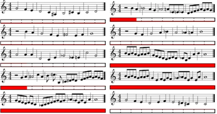
An example for some automatically generated melodies is given in figure 19.

Based on this preliminary experimental study we conjecture that decision trees seem to be good for au-tomatic classification on a comparative small number of example individuals. Neural networks are not

con-G4 4 ˘ ˇ ˇ ˘ ˇ 4ˇ ˘ 4ˇ ˇ ˘ ˘ G4₄ < ˇ ˇ Z˘ ˇ ˇ Z˘ 6ˇ Zˇ ^ˇ Zˇ ˇ ˇ ˇĽĽˇˇ ˇ ˇ ˇ G4 4 < ˇ ˇ ˘ ˇ ˇ \˘ ˇ ˇ ¯ G44 < ˇ ˇ ˘ ˇ 2ˇ ˘ 2ˇ 6ˇ ¯ G4 4 ˘ ˇ ˇ ˘ ˇ ˇ Z˘ 2ˇ 6ˇ ˘ ˘ G44 ˇ ˇ ˇ ˇ ˇ ˇ ˇČȡ ˇ ˇ ˇÏÏˇˇ ˇ ˇ ˇ ZˇÚÚ_{ˇ ˇ} ˇ ˇ ¯ G4 4< ˇ ˇ \˘ ˇ ˇ -ˇ` \-ˇ` (ˇ \ˇ \ˇ ˇ ˇ ˇ ˇ ˇŔŔˇˇ ˇ ˇ ˇ G44 ˇ ˇ ˇ ˇ ˇ ˇ ˇČȡ ˇ ˇ ˇ ˇ ˇ ˇ Zˇ Zˇ ˇ ˇ ˇ ˇ ňňˇ ¯ G4 4 ˇ ˇ ˇÏÏˇ ˇÎΡ ˇ Zˇ ˇ ˇŔŔˇˇ ˇ ˇ ˇ Zˇ Zˇ ˇ ˇ ˇ ˇ ¯ G44 ˘ ˇ ˇ ˘ ˇ ˇ ˘ 4ˇ 4ˇ ˘ ˘

Fig. 19: Automatically generated melodies using a pruned decision tree with 5 fitness classes in 20 generations. The bars specify the automat-ically assigned fitness.

vincing and should be analysed on a larger training set. With our method it is possible to generate pleas-ant melodies in just a few generations of an evolution-ary algorithm.

8 Future Work

One main task for future work is to generate a larger example set for analysing different methods for auto-matic classification in a more comprehensive manner. For that purpose it will be helpful to have many exper-iment participants for a not that subjective evaluation of the training melodies. Another point is the analysis of other similarity functions like the one mentioned in [7].

For the initialisation, an implementation of a com-bined Markov chain for rhythm and melody in one model shall be implemented which also respects the position of notes in the melody respectively in the cur-rent bar.

References:

[1] T. Bäck, D. B. Fogel, and Z. Michalewicz, ed-itors. Handbook of Evolutionary Computation. Institute of Physics Publishing and Oxford Uni-versity Press, Bristol, UK, 1997.

[2] J. A. Biles. Genjam: A genetic algorithm for generating jazz solos. InProceedings of the In-ternational Computer Music Conference (ICMC 1994), pages 131–137, San Francisco, USA, 1994. International Computer Music Associa-tion.

[3] J. A. Biles. Genjam populi: Training an iga via audience-mediated performance. pages 347– 348, San Francisco, USA, 1995.

[4] J. A. Biles, P. G. Anderson, and L. W. Loggi. Neural network fitness functions for a musical iga. InProceedings of the Soft Computing Con-ference (SOCO 1996), pages B39–B44, Reading, UK, 1996. ICSC Academic Press.

[5] A. R. Burton. A Hybrid Neuro Genetic Pattern Evolution System Applied to Musical Composi-tion. PhD thesis, University of Surrey, School of Electronic Engineering, Information Technol-ogy and Mathematics, Guildford, Surrey, Eng-land, 1998.

[6] W. S. Cleveland. LOWESS: A program for smoothing scatterplots by robust locally weighted regression. The American Statistician, 35:54, 1981.

[7] M. Grachten, J.-L. Arcos, and R. L. de Mántaras. Melodic similarity: Looking for a good abstrac-tion level. In Proceedings of the International Conference on Music Information Retrieval (IS-MIR), Barcelona, Spain, 2004.

[8] C. Igel and M. Hüsken. Empirical evaluation of the improved Rprop learning algorithms. Neuro-computing, 50:105–123, 2003.

[9] M. Iosifescu. Finite Markov Processes and Their Applications. John Wiley & Sons, Inc., Bucharest, Romania, 1980.

[10] B. Johanson and R. Poli. Gp-music: An interac-tive genetic programming system for music gen-eration with automated fitness raters. Technical Report CSRP-98-13, Stanford University, Uni-versity of Birmingham, 1998.

[11] R. Klinger. Komposition von Musik mit Meth-oden der Computational Intelligence. Master’s thesis, Department of Computer Science, Uni-versity of Dortmund, Germany, June 2006. [12] R. Klinger and G. Rudolph. Evolutionary

com-position of music with learned melody evalu-ation. In Proceedings of International Con-ference on Computational Intelligence, Man-Machine Systems and Cybernetics (CIMMACS ’06), Venice, Italy, 2006.

[13] E. R. Miranda. Composing Music with Comput-ers. Elsevier/Focal Press, 2001.

[14] G. Papadopoulos and G. Wiggins. AI methods for algorithmic composition: A survey, a critical view and future prospects. InSymposium on AI and Scientific Creativity (AISB’99): Symposium on Musical Creativity, pages 110–117, 1999.

[15] J. R. Quinlan. Induction of decision trees. Ma-chine Learning, 1(1):81–106, 1986.

[16] J. R. Quinlan. Learning with continuous classes. InProceedings of the Fifth Australian Joint Con-ference on Artificial Intelligence, pages 343– 348, 1992.

[17] M. Riedmiller and H. Braun. A direct adaptive method for faster backpropagation learning: the rprop algorithm. In Proceedings of the Inter-national Conference on Neural Networks, San Francisco, USA, 1993.

[18] G. Rudolph. An evolutionary algorithm for inte-ger programming. In Y. Davidor, H.-P. Schwefel, and R. Männer, editors,Parallel Problem Solving from Nature – PPSN III, pages 139–148, Berlin, Germany, 1994. Springer.

[19] M. Towsey, A. Brown, S. Wright, and J. Diederich. Towards melodic extension using genetic algorithms. In A. R. Brown and R. Wild-ing, editors,Proceedings of Interfaces: The Aus-tralian Computer Music Conference, pages 85– 91, 2000.

[20] G. M. Werner and P. M. Todd. Franken-steinian methods for evolutionary music com-position. In N. Griffith and P. Todd, editors,

Musical Networks: Parallel Distributed Per-ception and Performance, pages 313–339. MIT Press/Bradford Books, Cambridge, USA, 1998. MIT Press/Bradford Books.

[21] G. Wiggins and G. Papadopoulos. A genetic al-gorithm for the generation of jazz melodies. In

Proceedings of the Finnish Conference on Artifi-cial Intelligence (STeP ’98), Jyväskylä, Finland, 1998.

[22] I. H. Witten and E. Frank.Data Mining. Elsevier Inc., San Francisco, USA, 2005.

[23] I. Xenakis. Formalized Music – Thought and Mathematics in Composition. Indiana University Press, Bloomington, Indiana, USA, 1971.