Loudspeaker crossover networks

(1)

Loudspeaker crossover networks

By Tore A. Nielsen

Student 041915 at DTU, the Technical University of Denmark August 2005

Abstract

Loudspeaker systems use crossover networks directing low and high frequencies to individual loudspeaker units optimised for limited frequency ranges. The introduction of a crossover network should not degrade the resultant performance but the loudspeakers are physically separated, which introduces problems around the crossover frequency when listening off-axis, and the individual responses of the loudspeaker units further complicates summation of the output signals. The front baffle introduces reflections from the edges and the listening room adds reflections from its boundaries causing interference with the direct signal seriously affecting the resultant response of the loudspeaker system.

The objective of this report is the study of crossover networks and the different causes that degrades the performance.

(2)

Contents

1. Introduction ... 5 1.1. Crossover network ... 5 1.2. Threshold of hearing ... 6 1.2.1. Audible range ... 6 1.2.2. Change of level ... 6 1.2.3. Group delay ... 7 1.3. Musical instruments ... 7 1.4. Cut-off slope ... 8 1.5. Transfer function ... 9

1.5.1. Ideal filters – Constant voltage filters ... 10

1.5.2. Non-ideal filters – All-pass filters ... 11

1.5.3. Butterworth filters ... 13

2. Crossover networks ... 15

2.1. First-order ... 15

2.1.1. Symmetrical – two way ... 15

2.1.2. Using bass loudspeaker roll-off ... 17

2.2. Second-order ... 19

2.2.1. Asymmetrical – two way ... 19

2.2.3. Symmetrical – three way... 22

2.2.4. Steep cut-off – two way ... 24

2.3. Third order... 27

2.3.1. Asymmetrical – two way ... 27

2.4. Fourth order ... 34

2.5. Passive network ... 37 2.5.1. First order ... 37 2.5.2. Second order ... 38 2.5.3. Third order ... 38 2.5.4. Fourth order ... 39 2.5.5. Loudspeaker impedance ... 40 2.6. Active network ... 42 2.6.1. First order ... 43 2.6.2. Second order ... 43 2.6.3. Higher orders ... 43 2.6.4. Special ... 44 3. Models ... 46 3.1. Electro-acoustical model ... 46

3.1.1. The loudspeaker unit ... 47

3.1.2. Electrical circuit ... 49

3.1.3. Mechanical circuit ... 50

(3)

3.1.5. Diaphragm velocity ... 54

3.1.6. Sound pressure ... 57

3.2. Loudspeaker pass band ... 59

3.2.1. Sound pressure level ... 59

3.2.2. Diaphragm excursion ... 60

3.2.3. SPICE simulation model ... 61

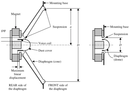
3.3. Directivity ... 62 3.4. Diffraction ... 63 3.4.1. Circular baffle ... 63 3.4.2. Sectional baffle ... 65 3.4.3. Square baffle ... 66 3.5. Listening angle ... 69 3.5.1. Two loudspeakers ... 69 3.5.2. Three loudspeakers ... 71 3.6. Boundary reflection ... 73

3.6.1. One reflecting surface ... 73

3.6.2. Rectangular room ... 75 3.6.3. Home entertainment ... 77 3.6.4. Public address ... 80 3.7. Loudspeaker characteristics ... 81 3.8. Group delay ... 82 3.8.1. Calculation method ... 82 3.8.2. Implementation in MATLAB ... 82 3.8.3. Verification... 83

4. Assembling the models ... 86

4.1. Loudspeaker models ... 86 4.2. Crossover network ... 86 4.3. Angular response ... 89 4.4. Reflections ... 90 4.5. Conclusion ... 91 5. References ... 92 5.1. Books ... 92 5.2. Papers ... 92 5.3. Links ... 92 6. Appendix ... 93

6.1. Plot transfer function ... 93

6.1.1. Main script ... 93 6.1.2. Filter function ... 96 6.1.3. Loudspeaker ... 96 6.1.4. Directivity ... 97 6.1.5. Diffraction ... 97 6.1.6. Boundary reflections ... 97

(4)

Foreword

The current project was initiated as a three-week course to be executed in August of the 2005 summer vacation since I could not participate in the normal three-week period in June. My professor Finn Agerkvist accepted the proposal of a project to study crossover networks.

The main objective was the design of crossover networks realising a transfer function of unity, i.e. flat amplitude and zero phase, and I planned to include the effect of loudspeaker bandwidth, the problems associated with off-axis listening due to the displacement of the loudspeaker on the front baffle and the interference from reflections within the listening room. Finn Agerkvist suggested that I also included the reflections due to diffraction.

Initially I planned to use SPICE for simulations and a spread sheet for calculations, but I soon realised that it was more appropriate to base the simulations and calculations on MATLAB.

I decided to work through the loudspeaker model presented by Leach in order to derive a useful model for loudspeakers, and I included the effect of the voice coil inductance and combined the low and high frequency models from Leach into one single model, which covers the frequency range below diaphragm break-up.

As the project progressed, I realised the need to include group delay and it seemed appropriate to add notes on the threshold of hearing thus defining an acceptance limit for use during the development of a crossover network. According to my log, I have been working for 180 hours, which is 50 % more than the nominal workload for a three-week course. If an unlimited amount of time were available, I would have worked more on high-order crossover filters and improved the sections on diffraction, off-axis listening, boundary reflection and group delay.

Tore A. Nielsen August 14, 2005.

(5)

1. Introduction

Ideally, a single loudspeaker should reproduce the full audible frequency range without any detectable distortion, but this is unfortunately not possible although good full-range loudspeakers do exist. The frequency range of a full-range loudspeaker is limited with weak bass and unsatisfactory treble, the frequency response is irregular or at least compromised by the directivity at high frequencies and it is difficult to keep distortion low when the same diaphragm is used for bass and treble.

Low frequencies moves the diaphragm significantly at high sound pressure levels thus introducing harmonic distortion related to loudspeaker construction (magnet, voice coil and suspension) and inter-modulation between bas and treble caused by the Doppler-effect. The one and only way of distortion reduction is decreasing diaphragm excursion, but this require an increase of diaphragm area to compensate for the lost sound pressure; and enlarging loudspeaker size worsens high frequency reproduction.

It all boils down to a requirement of loudspeakers optimised for reproduction of a limited frequency range and thus the need of a frequency dividing network.

1.1. Crossover network

A pair of typical crossover networks are shown in Figure 1. To the left is a two-way system, which could use a crossover frequency around 2 kHz, and to the right is a three-way system, which could use crossover frequencies around 800 Hz and 4 kHz.

High-pass filter Low-pass filter High-pass filter Band-pass filter Low-pass filter High-frequency loudspeaker (Treble) Mid-frequency loudspeaker (Midrange) Low-frequency loudspeaker (Bass) PA PA PA PA Audio source Audio source

Figure 1 – Layout of a typical cross-over network, which can be passive, i.e. consisting of capacitors, inductors and resistors and driven from a single power amplifier (left), or it can be active, i.e. using operational amplifiers with frequency-dependent feedback and individual power amplifiers for each channel (right).

The loudspeakers are driven from power amplifiers, which can either be located before the crossover network; the conventional approach using passive crossover networks, or the power amplifier can be located between the crossover network and the loudspeaker; thus requiring an amplifier for each loudspeaker.

The passive crossover network is currently the most used approach but the active crossover network is expected to be increasingly popular in the near future since high-quality power amplifier modules based upon the switch-mode technique (Class D) are becoming a serious alternative to the linear power amplifiers of today. In addition to improved control of filter parameters and protection of the loudspeakers do the active crossover network offer electrical control of the moving system parameters and adjustment of the response to the listening room.

But before entering the study of crossover networks, a few words on what can be heard, and what cannot, is required.

(6)

1.2. Threshold of hearing

There is no idea in optimising a filter if the improvement is inaudible and the money could be spend better on other jobs. So, here is a brief overview of what is audible and what is not. Don’t take the limits too literately; they are meant as guidelines.

1.2.1. Audible range

The audible range is defined by the Fletcher-Munson curves reproduced to the left in Figure 2. They published their data in 1933 using headphones; measurements using anechoic chambers were published in 1956 by Robinson-Dadson and later reviewed and standardised in 2003 as ISO 226, shown to the right.

Figure 2 – Equal loudness contours due to Fletcher-Munson (http://en.wikipedia.org) and to Robinson-Dadson (http://www.aist.go.jp/aist_e/latest_research).

We can hear signals from 15 Hz to 15 kHz but few loudspeaker systems can reproduce this range, at least not at realistic levels since low-frequency signals require large diaphragms and long voice coils in order to move the air; the sound pressure level must exceed 80 dB at very low frequencies to be heard and 110 dB is required at 20 Hz to balance a typical speech level around 65 dB.

Organ music may extend to 16 Hz for organs fitted with 32 feet pipes, but they are rarely found – and rarely used – so organs music is limited to 32 Hz. Piano music may extend to 27 Hz, while jazz, rock and popular music seldom passes below 41 Hz; the lowest string on the acoustical double bass and the electric bass guitar. Powerful low-frequency signals may, however, arise from electrical keyboards, computerized effects and recordings of large drums, machines, thunder storms and explosions.

No one can hear sound above 20 kHz, and aging further reduces the limit, so a pragmatic upper limit would be 15 kHz. People with “golden ears” may postulate that the treble unit should extend far beyond 20 kHz to avoid phase distortion. The audibility of phase is controversial, so a safe view would be that reproduction beyond 20 kHz do not harm; but have in mind that FM-radio broadcasting limits the range to 15 kHz and CD-recordings to 20 kHz. Modern signal transmission using MPEG and other formats often use the 44.1 kHz sampling frequency of the CD-media thus sharing the limit.

1.2.2. Change of level

The ability to detect a change of level is between 0.5 dB and 2 dB [1] so loudspeaker artefacts below this limit can be expected inaudible. This is quite fortunate, since

(7)

irregularities of this order of magnitude must be expected with loudspeakers. It is obvious that the lowest limit should be used designing high-end equipment, since the listener can be expected to have trained ears.

1.2.3. Group delay

Threshold of audibility of group delay is being debated, but it should be relatively safe stating the limit as a couple of milliseconds for signals in the 500 Hz to 8 kHz range. (Source: http://www.trueaudio.com/post_010.htm).

1.3. Musical instruments

The fundamental note of musical instruments is typical located below 1 kHz as shown in Figure 3. The harmonic overtones extend beyond the hearing limit but the level is reduced toward the higher frequencies. The decay is strongly dependent upon the actual instrument being examined, but an average slope would be around –6 dB/octave. Most music use fundamentals within the 3½ octave range from the lower C-note at 65 Hz to the upper g2-note at 780 Hz, so the musical power is mainly restricted to this range.

10 Hz 100 Hz 1 kHz 10 kHz String quartet Human voice Brass ensemble Wood wind Piano Organ Orchester Dynamic range 50 dB 50 dB 35 dB 35 dB 70 dB 50 dB 50 dB

Figure 3 – Frequency range for the fundamental note of musical instruments [5].

The dynamic range extend from 40 dB to 110 dB for acoustical instruments and higher for electrically amplified music. A symphony or rock orchestra cannot be reproduced at realistic levels for home entertainment, so the playback level must typically be reduced. Recording level was previously compressed manually by increasing the weakest levels during recording, in order to cut the master disk (LP records) keeping the weakest signals above the noise floor of the medium. This is not needed nowadays for recording of compact disks (CD), where the dynamic level is, at least theoretically, 96 dB.

Reducing the reproduction level moves the weakest signals below the threshold of hearing, at least for the lowest frequencies, so the loudspeaker system may require a bass boost for reproduction at reduced levels. This is sometimes called physiological loudness contour and is included with many amplifier systems. The success of this correction is dependent upon the set-up of the combined system, consisting of the source, the amplifier, the loudspeaker and the size of the room and is most effectively implemented with integrated systems where the interconnection levels are known. The correction is often accompanied by a treble boost as well, but this is based on a misinterpretation of the equal loudness contour; the treble part of the equal loudness contour is turned upward at high frequency thus indicating reduced sensitivity at high frequencies, but the distance between the different levels is almost constant so correction is not required.

(8)

1.4. Cut-off slope

A crossover network is not a brick wall filter with infinite attenuation outside the pass band; the crossover network gradually attenuates the signal above or below the crossover frequency as illustrated in Figure 4 for low-pass and high-pass filters.

The pass band is the frequency range where attenuation is minimum, typically –3 dB although some filters attenuate more than this. The transition band is the frequency range where the attenuation is becoming active and the stop band is the frequency range where the attenuation has become sufficient to efficiently remove the loudspeaker.

Figure 4 – Filter characteristics for Butterworth filters with orders 1, 2, 3, 4 and 6.

A loudspeaker contributes with audible output in the transition band, which must be taken into account to avoid interference between the loudspeakers. Sufficient amount of attenuation is obtained when the level from the attenuated channel is less than a certain limit, for instance below –20 dB. The limit defines the acceptable interference level.

Assume for example, that the loudspeaker peaks 6 dB at some frequency near the stop band and that this must be attenuated. With –20 dB of intended attenuation this corresponds an actual level of –14 dB, or a sound pressure of 10-14/20 = 20 % of the nominal level, which may result in ±2 dB of interference.

A crossover network with a cut-off slope of ±6 dB/octave indicates that the loudspeaker must be well-behaved for at least 3 octaves beyond the cross-over frequency. A bass loudspeaker, which is to be cut-out above 2 kHz, must be reasonably flat to 16 kHz. The crossover network must protect the treble loudspeaker from the high power levels at lower frequencies. The loudspeaker is compliance-controlled below the resonance frequency, which is usually around 1 kHz, so the diaphragm moves in proportion to the applied voltage. The low-frequency excursion of the diaphragm may be inaudible but it may give rise to audible distortion of high-frequency signals when the low-frequency excursion of the suspension system reaches the non-linear region. The unnecessary dissipation of power heats the voice coil and may damage the treble loudspeaker, which is capable of handling few watts only.

Most of the signal power in music is located below approximately 500 Hz so a power reduction well below 1 W of dissipation within the treble loudspeaker requires in excess of 20 dB of attenuation for sufficient protection. If the treble loudspeaker is to be cut-in at 2 kHz, which is just two octaves above 500 Hz, the required filter slope becomes a minimum of 12 dB/octave.

(9)

1.5. Transfer function

All channels of the crossover network will be described by their transfer function, which is a convenient way of describing an electrical filter, and system analogies allow straightforward transformation to mechanical and acoustical systems as well. The transfer function may be defined from requirements such as flat amplitude, which can then be used to specify the system parameters.

Bandwidth-limited channel #1 H1 Input signal Bandwidth-limited channel #2 H2 + + Output signal EOUT = (H1 + H2)EIN EIN EOUT1 = H1EIN EOUT2 = H2EIN Σ

Figure 5 – A crossover network consists of two or more filter channels dividing the frequency range between the loudspeakers. The output from the loudspeakers are summed at the observation point; i.e. at the ear of the listener.

Transfer functions will be expressed in the frequency domain where frequency is represented by the Laplace operator s, defined by: s = α + iω. The initial conditions are

described by α and ω = 2πf is the angular frequency. Throughout this report is α = 0, so s = iω can be assumed although the formulas are generally valid and may, if required,

be transformed to the time domain using the inverse Laplace transform. However, time domain representations are not referenced in this document.

The complex frequency operator will be normalised by division with ω0, which

represents the cut-off frequency in most situations.

0

0 _ω

s

s =

A transfer function H is defined by the excitation input to the network, EIN, and the

output response from the network, EOUT. Assuming sinusoidal excitation:

( )

i t HE

HE

E_OUT = _IN = 0exp ω

An input excitation signal EIN is routed in parallel to the channels of a network with the

individual transfer functions H1, H2, ... and the output signals become:

... , , 2 2 1 1 IN OUT IN OUT H E E H E E = =

The loudspeakers will, for the moment, be considered ideal, so the acoustical output of the loudspeaker is a true copy of the electrical input signal. Assuming linearity, the signals from the individual channels are added at the receiver:

K + + = OUT1 OUT2 OUT E E E

Using the above definition of the transfer function, the sum can be written:

(

M

)

IN

OUT H H H E

E = + +K+

2 1

The sum of the individual transfer functions is defined as the system transfer function.

H H

H

(10)

The main objective of this report is analysing the system transfer function for the complete system involving the crossover network, the loudspeakers, the front baffle and the listening room. In order to do so, a reference transfer function is needed for comparison. It is obvious, that an ideal transfer function should not add or remove any information, it should be a string of wire.

1 =

H

A scaling factor, different from unity, is allowed, since amplification, attenuation, sign inversion or time delay within the system is not considered a distortion of the signal. The scaling factor may also include a dimension for transformation between the electrical, mechanical or acoustical systems.

1.5.1. Ideal filters – Constant voltage filters

Although loudspeakers are far from ideal, avoiding approximations in the design of the crossover network it is a good starting point. The design of crossover networks fulfilling the requirement H = 1, which guarantees flat amplitude and a phase of zero, are called constant-voltage filters and will be based upon the following polynomial:

N N N N as a s a s s P 0 1 0 1 2 0 2 0 1 1+ + + + + = − − L

The constants a1, a2, …, aN-1 defines the filter type, N is the order of the polynomial and

the coefficients are shown for the Butterworth filter type later in this chapter. Other polynomials, such as Bessel or Chebychev, can use the above polynomial form if they are normalised to unity for coefficients a0 and aN. If this is not the case, all terms of the

polynomials must be divided by a0, and the normalisation coefficient ω0 must thereafter be

corrected to include a0 and aN.

An alternative representation of PN is the product form, which is using the roots of the

polynomial.

The third order Butterworth polynomial can be represented by the following two identical expressions: ( 0) ( 0) ( 0) 3 3 0 2 0 0 3 866 . 0 5 . 0 866 . 0 5 . 0 1 2 2 1 s i s i s P s s s P + − × + + × + = + + + =

After the multiplications are carried out the original polynomial results. A transfer function of order N can now be defined:

N o N N N o N N N N N s s a s a s a s s b s b s b P Q H + + + + + + + + + + = = ₋ − − − 1 0 1 2 0 2 0 1 1 0 1 2 0 2 0 1 1 1 L L

The transfer function satisfy the requirement H = 1 when ai = bi since the nominator

polynomial QN and denominator polynomial PN are identical, but the requirement will

be violated, if ai ≠ bi for one or more of the terms. This violation may be required

building crossover networks of high order where the ideal transfer function becomes cumbersome. The result is anyway a valid transfer function although the phase response and possibly also the amplitude response will be affected.

(11)

Division into crossover channels uses the following identity: N N N N N N N N N P s P s b P s b P s b P H 0 1 0 1 2 0 2 0 1 1 ₊ ₊ ₊ ₊ ₊ = _L − −

Each term represents a transfer function with its own characteristics and two or more terms can be combined as required. All terms share the same denominator polynomial and are thus of the same order, regardless of the actual order of the nominator.

Two examples will introduce the method.

Example 1. For a first-order crossover only two terms are available so the design leaves no choice other than accepting the following arrangement:

0 0 1 0 1 0 1 1 1 1 1 s s P s H s P H HP N LP = = ₊ = = ₊

Example 2. For a crossover network of sufficiently high order (N≥ 4), the first two terms of PN can be used for the bass channel, the last two terms for the treble channel and the

remaining terms are available for the midrange channel:

N N N N HPN N N N BPN N LPN P s s b H P s b s b H P s b H 0 1 0 1 2 0 2 2 0 2 0 1 1 + = + + = + = L − − − −

The cut-off slopes are proportional to 1/fN-1 for the bass channel, fN-1 for the treble channel and f2 and 1/f2 for the midrange channel. A fourth order filter would offer cut-off slopes of ±18 dB/octave for bass and treble and ±12 dB/octave for midrange.

Both filters are realised in the next chapter together with other implementations.

1.5.2. Non-ideal filters – All-pass filters

The above method is useful for filters up to fourth order but become cumbersome for higher orders. A solution is to remove all middle terms and use only the first and last terms representing the low-pass and high-pass channels. These filters, which are called all-pass filters, can be used for crossover networks of any order. The requirement H = 1 is not satisfied so the phase of the filter will be different from zero.

With b1, b2, … , bN-1 set to zero the transfer functions become:

N N N N N HPN N LPN P s H P s H and P H = 1 = 0 _⇒ =1+ 0

The first term represents a low-pass channel with a cut-off frequency of f0 = ω0/2π and a

cut-off slope of 1/fN, so the higher frequencies are attenuated by –6N dB/octave. Filter amplitude response is flat under certain conditions, which will be analysed below. First-order filters are ideal (constant-voltage filters) and will not need special considerations.

N s N s N LPN s P P H 0 0 1 1 1 1 0 0   →  =   →  = ∞ → →

The second term represents a high-pass channel with a cut-off frequency of f0 = ω0/2π

and a cut-off slope of fN, so the lower frequencies are attenuated by 6N dB/octave.

Frequency Amplitude

f0

-6N dB/octave 1

(12)

1 0 0 0 0 0 0 0 0 =   →  =   →  = ∞ → → N N s N N N s N N HPN s s P s s P s H

When the output from both channels are combined the following transfer function for the complete system is obtained:

N N N N N N P i H crossover At P s H =1+ 0 : =1+

At crossover (s0 = i) is the sum depending upon the filter order and for N = 2, 6, 10, ...

the terms cancel – no signal is being transmitted at crossover. The cancellation can be avoided by sign inversion one of the channels, which has the consequence that the phase moves from 0° to –180° through the frequency range.

• For N odd are the channels 90° or 270° out of phase, and the channels combine at crossover with 3 dB of loss. To avoid peaking, the transfer functions must be designed to –3 dB at the crossover frequency and this can be realised using a Butterworth polynomial as basis for the design.

• For N even are two channels in-phase if the above mentioned sign inversion is included as required and the channels combine at crossover without loss. To avoid peaking, the transfer functions must be designed to –6 dB at the crossover frequency. This can be realised using a squared Butterworth polynomial as basis for the design; a design method referred to as the Linkwitz-Riley filter design. Constant amplitude, |HN| = 1, is realised by the so-called all-pass filters, which are

based upon the Butterworth polynomials.

First-order crossover networks are born as ideal filters (i.e. constant voltage), so the amplitude is constant. This will be demonstrated below using variable w = ω/ω0 as a

substitute for s0 in order to identify real and imaginary parts of the frequency variable.

The all-pass variant of the first-order crossover network (1 – s0 in the nominator) is also

useful and is analysed as well [2].

1 1 1 1 1 1 1 2 2 2 2 0 0 1 = + + = + ± = + ± = w w iw iw s s H

Filters of higher order can realise the all-pass function when the polynomial used is of Butterworth characteristic, since this allows factorisation of the nominator and denominator polynomials.

Second-order crossover networks require inversion of the high-pass channel to avoid the notch filter and the level must be –6 dB at crossover, so the crossover network is based on a squared first-order Butterworth polynomial. The amplitude response becomes [2]:

(

)

(

)(

)

1 ₁1 1 1 1 1 1 1 1 1 1 1 2 2 2 2 0 0 0 0 0 0 2 0 2 0 2 = + + = + − = + − = + + − + = + − = w w iw iw s s s s s s s s H Frequency Amplitude f0 6N dB/octave 1

(13)

Third-order crossover networks are insensitive to the sign of the treble channel (the amplitude response is unaltered although the phase response is changed). The third-order Butterworth polynomial use a1 = a2 = 2, and the factorisation results in [2]:

(

)

(

)

(

)

(

)

(

)

(

)

(

)

(

)

(

)

1 1 1 1 1 1 1 1 1 2 2 1 1 1 1 1 1 1 1 1 1 1 2 2 1 1 2 2 2 2 2 0 0 0 2 0 0 0 3 0 2 0 0 3 0 3 2 2 2 2 2 2 2 2 0 0 0 2 0 0 0 3 0 2 0 0 3 0 3 = + + = + − = + + + + + − = + + + − = = + − + − = − + − − = + + + + − + = + + + + = w w iw iw s s s s s s s s s s H w w w w w iw w iw s s s s s s s s s s H

Fourth-order crossover networks require a level of –6 dB at crossover and can be based upon a squared second-order Butterworth polynomial (a1 = √2). The amplitude response

becomes [2]:

(

)

(

)(

)

(

)

(

1

)

1 1 2 1 2 1 2 1 2 1 2 1 2 1 2 1 2 1 1 2 2 2 2 2 2 2 0 0 2 0 0 2 2 0 0 2 0 0 2 0 0 2 2 0 0 4 0 4 = + + = + + + − = + + + − = + + + − + + = + + + = w w w w i w w i s s s s s s s s s s s s s H

Higher order filters are not covered in this report but can, according to reference [2], be shown to fulfil the all-pass filter requirement H = 1.

1.5.3. Butterworth filters

Crossover networks are often based upon the Butterworth polynomial since this leads to good all-pass filters. The amplitude response for a Butterworth low-pass filter is [5]:

1 1 1 1 1 0 0 2 0 2 0 0 0   →          →        + = + = → ∞ → s N s N N LPN s H ω ω ω ω

The amplitude approaches unity for zero frequency, the amplitude is 1/√2 or –3 dB at the crossover frequency regardless of the filter order, and the asymptotic cut-off slope for higher frequencies is –6N dB/octave. This is a maximally flat filter and one of its characteristics is, that all filter blocks of the physical implementation will be designed for the same cut-off frequency but with different quality factors.

Other filter characteristics are realised through frequency transformation, introduced briefly below [5], but the transformations are not required for the current analysis since the different channels are generated directly from the transfer function and not from transformation of a model filter.

(14)

A high-pass filter is realised by transformation of s0 into 1/s0: N s s N N HPN s H s s         →    →        + =       + = ⇒ → → ∞ → 0 0 2 0 2 0 0 0 0 0 1 1 1 1 1 1 1 ω ω ω ω

A band-pass filter is realised by the following transformation, which consists of 1/s0 as

well as s0 in combination with a coefficient B, representing the bandwidth of the

resulting filter: N N N s i s N N N s N BPN B Bs B B s Bs s H Bs s s       =         →   →        =         →        ₊ + = ⇒ + → → = ∞ → 0 0 0 0 0 2 0 2 0 0 2 0 0 1 1 1 1 1 1 1 1 0 0 0 ω ω ω ω

The coefficients and roots of the Butterworth polynomial is shown in the table below for filters from second to seventh order. The first-order polynomial 1 + s0 is Butterworth

too but do not include coefficients to be defined.

Table 1 – Coefficients and roots of Butterworth polynomials (from [5]).

Order Coefficients Roots

2 a1 = 1.4142 (-0.7071 ±i0.7071) 3 a1 = a2 = 2.0000 (-1) (-0.5000 ±i0.8660) 4 a1 = a3 = 2.6131 a2 = 3.4142 (-0.3827 ±i0.9239) (-0.9239 ±i0.3817) 5 a1 = a4 = 3.2361 a2 = a3 = 5.2361 (-1) (-0.3090 ±i0.9511) (-0.8090 ±i0.5878) 6 a1 = a5 = 3.8637 a2 = a4 = 7.4641 a3 = 9.1416 (-0.2588 ±i0.9659) (-0.7071 ±i0.7071) (-0.9659 ±i0.4339) 7 a1 = a6 = 4.4940 a2 = a5 = 10.0978 a3 = a4 = 14.5918 (-1) (-0.2225 ±i0.9749) (-0.6235 ±i0.7818) (-0.9010 ±i0.4339)

(15)

2. Crossover networks

Ideal filters, defined by the transfer function requirement H = 1, were expected to realise good crossover networks but this proved to be the case only for low-order networks; higher order networks tend to include terms complicating the construction and obstructing the operation. All-pass filters, realising two-way systems with maximum cut-off slope, were also analysed and proved to operate as expected.

2.1. First-order

Crossover networks of first order are popular because the component cost is low; it may sometimes be possible designing crossover networks with one single capacitor for the treble loudspeaker. However, the cut-off slope is ±6 dB/octave, which is insufficient in most cases since the loudspeakers must reproduce well 3 octaves past the crossover frequency. This is problematic since bass loudspeakers suffer from increased directivity and diaphragm break-up at high frequencies, which concentrates the sound on-axis and typically generates a ragged high-frequency response, and treble loudspeakers cannot reproduce below the resonance frequency.

In addition to this is the filter insufficient in protecting the treble loudspeaker against destructive low-frequency signals, so the first-order crossover is limited to loudspeakers intended for low sound pressure levels and is typically found in low-cost designs. A first-order transfer function is defined from HN with N = 1:

0 0 1 1 1 s s H + + =

2.1.1. Symmetrical – two way

The equation is separated into two channels with a low-pass channel for the bass loudspeaker and a high-pass channel for the treble loudspeaker.

0 1 0 0 1 1 1 1 s H s s H LP HP + = + =

Realisation is simple, only one component is required for each branch but the filter is

very dependent upon the impedance of the loudspeaker so the passive network may not prove satisfactory in real life.

Bass REB

LB1 CT1

Treble RET

Figure 6 – Passive crossover network. The attenuation is as expected only when the impedance of the loudspeakers are constant, so impedance compensation is required in most cases – hence opposing the simplicity of the design.

(16)

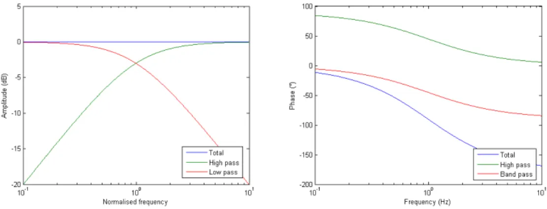
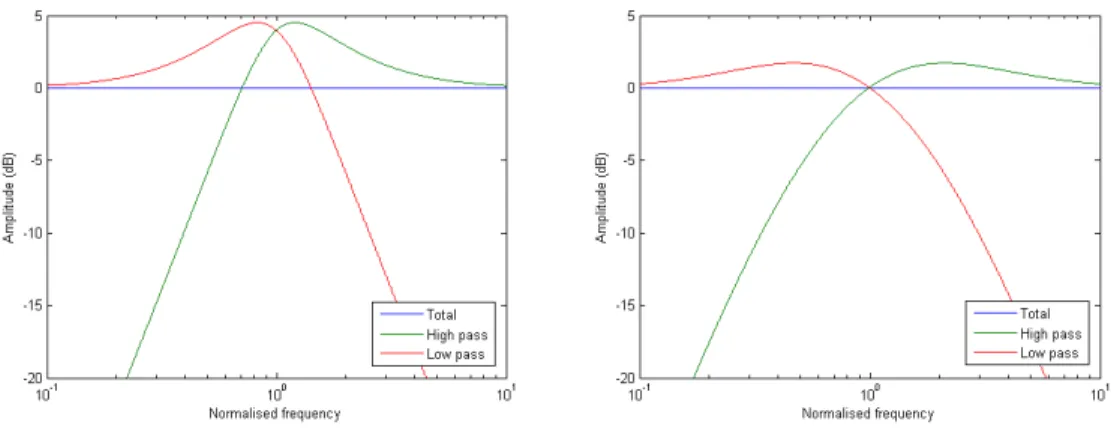
The result is shown below. The channels add up to unity and the phase to zero, as they should since this is an ideal filter (constant-voltage) and assuming perfect loudspeakers with identical path lengths to the listener.

Figure 7 – Amplitude and phase response. The loudspeakers are 90° out of phase throughout frequency, thus adding with 3 dB of loss when combined. The channels are at –3 dB at crossover and add to 0 dB.

A variant of the filter is realised by inverting the treble loudspeaker, which generates the following transfer function:

0 0 1 1 1 s s H + − =

This is an all-pass filter, where the amplitude is flat but the phase is changing gradually from 0° to –180° through frequency with –90° at crossover.

Figure 8 – Amplitude and phase response with the treble loudspeaker inverted. The loudspeakers are 90° out of phase throughout frequency.

The introduction of a phase different from zero for the complete crossover network introduces a group delay different from zero and this is shown in Figure 9.

Note that the group delay unit is calculated for a normalised filter corresponding to a cut-off frequency of 1 Hz. With a cut-off frequency of 1000 Hz the group delay scaling will be in milliseconds and not seconds.

(17)

Figure 9 – Group delay with the treble loudspeaker inverted.

2.1.2. Using bass loudspeaker roll-off

Some bass loudspeakers are designed to roll off smoothly above a certain frequency, typically in the range where the crossover frequency is placed. The crossover network can be simplified if this roll off is used as the low-pass filter thus only implementing the high-pass filter capacitor for the treble loudspeaker. This results in a low-cost crossover network since only one capacitor is required. The bass loudspeaker must realise the required transfer function, so the –3 dB frequency of the bass loudspeaker dictates the crossover frequency. Bass RE CT1 Treble RE

Figure 10 – Passive crossover network using the bass loudspeaker roll off.

Treble loudspeakers build from piezoelectric transducers with an integrated horn are available with a cut-off frequency of approximately 4 kHz and can be used without external components. The treble loudspeaker accepts up to 30 V applied directly and can be used for a two-way system without any components within the crossover network – but the cut-off is very sharp so the resulting design is not a first-order crossover network.

It is possible to electrically adjust the cut-off frequency of the bass loudspeaker using

pole-zero compensation, which is most effectively implemented using active filtering. The method can be used to “move” the bass loudspeaker voice coil cut-off frequency from the actual value to the desired value.

Assume that the bass loudspeaker cut-off frequency is at ω1, and not at ω0 as required.

The transfer function can be rewritten to include a null and a pole at the new frequency. The ratio of the new null/pole transfer function is unity so the transfer function is not changed.

(

)(

)

1 1 1 0 1 1 1 0 0 1 1 1 1 1 1 1 1 1 1 LS CN LP H H s s s s s s s H = + + + = + + × + = + =

(18)

The terms are then arranged so the zero is moved to the crossover network HCN1. The

transfer functions for the crossover network HCN1 and the bass loudspeaker HLS1 then

becomes: 1 1 0 1 1 1 1 1 1 s H s s H_CN _LS + = + + =

The crossover network HCN1 is now a correction filter, which modifies the amplitude

spectrum of the low-frequency channel making the bass loudspeaker useful with the required crossover frequency. The correction should not be brought too far, however, but minor corrections of the order of ±6 dB (one octave up or down) should be realisable.

Note, that moving the crossover frequency upward requires amplification of the signal fed to the bass loudspeaker and moving the crossover frequency down requires attenuation of the signal fed to the bass loudspeaker. The former is impossible to implement using passive filters and the latter impractical, hence the recommendation of active filtering.

(19)

2.2. Second-order

Crossover networks of second order are popular due to the low component count and relatively steep cut-off slope. In addition is the designer provided with an interesting collection of filters to select among; both the ideal constant-voltage and the non-ideal all-pass filters are offered.

A second-order transfer function is defined from HN with N = 2: 2 0 0 1 2 0 0 1 2 1 1 s s a s s a H + + + + =

Coefficient a1 defines the filter characteristic around the crossover frequency and is

conventionally defined by the quality factor Q of a second-order circuitry:

Q a1= 1

A common quality factor is 0.71 for the Butterworth characteristic, which is –3 dB at the crossover frequency, but any value can be used with Q = 0.5 to 1 as typical values.

2.2.1. Asymmetrical – two way

One obvious realisation of a two-way crossover network is to divide between the first-order and second-first-order terms thus increasing the cut-off slope for the treble loudspeaker to improve the protection.

2 0 0 1 0 1 2 2 0 0 1 2 0 2 1 1 1 s s a s a H s s a s H LP HP + + + = + + =

The high-pass filter is of second-order with a slope of 12 dB/octave, which is sufficient to protect the treble loudspeaker. A useful range of 1.5 octaves below the cut-off frequency is required for 20 dB of attenuation so the crossover frequency must be higher than 21.5 = 2.83 times the resonance frequency of the treble loudspeaker.

At the crossover frequency, and assuming a1 = 2, we get:

° − ∠ = − = + = − + + = ° ∠ = = − = − + − = 27 1 . 1 1 2 2 1 1 2 1 2 1 90 5 . 0 2 1 1 2 1 1 2 1 2 2 1 2 i i i i i H i i i H LP HP

So, the channels are 117° apart and will add with some loss, hence the slight boost of the low-frequency channel at the crossover frequency. For a1 = 1 both channels are

boosted but the sum remains constant at unity so the phase of the channels are moved further apart for reduced value of a1. This is not a good way of designing a crossover

network; the channels should not oppose each other since the result then becomes a difference between two fighting channels. A sound way of designing is to select a fairly large value of the coefficient, where a1 = 2 seems to be a fair compromise.

(20)

Bass REB LB1 CT1 Treble RET LT1 RB1 CB1

Figure 11 – Passive crossover network.

Active realisation:

2

2 1 HP

LP H

H = −

The transfer function HHP2 is implemented as a standard second-order high-pass filter

with Q = 1/a1, and the low-pass channel can be derived by an operational amplifier. A

value of a1 = 1 results in Q = 1, which is a 1 dB Chebychev characteristic with relative

steep cut-off and this also applies to the low-pass channel, which is cut-off after one decade. A value of a1 = 2 results in Q = 0.5, which is the limit where the roots of the

polynomial becomes real. This removes any tendency to oscillate in the treble channel, hence the smooth transition without peaking. The cut-off of the low-pass channel is somewhat weaker so the bass loudspeaker must operate well to at least twenty times the cut-off frequency.

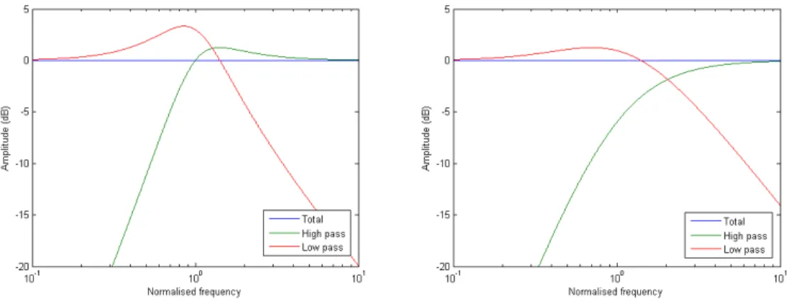
Figure 12 – Amplitude response with a1 = 1 (left) and a1 = 2 (right). The quality factor refers to the treble channel and is Q = 1 (left) and Q = 0.5 (right).

The low-pass filter is second-order but the first-order term in the nominator reduces the cut-off slope to –6 dB/octave at high frequencies, which requires a bass loudspeaker capable of operating 3 octaves above the cut-off frequency, so the channel is more or less full range and the bass loudspeaker must perform well at high frequencies.

(21)

2.2.2. Symmetrical – two way

The first-order term of the transfer function can be split into two halves so both channels includes a first-order term.

2 0 0 1 0 1 2 2 0 0 1 2 0 0 1 2 1 2 1 1 2 s s a s a H s s a s s a H LP HP + + + = + + + =

Both filters are of second-order but the slope is ±6 dB/octave, which is insufficient to protect the treble loudspeaker so the solution should not be used for high-power systems. The loudspeakers must be capable of operating 3 octaves outside the crossover frequency

At the crossover frequency, and assuming a1 = 2, we get:

° − ∠ = + = − + + = ° ∠ = − = − + − = 45 71 . 0 2 1 1 2 1 1 45 71 . 0 2 1 1 2 1 1 2 2 i i i i H i i i i H LP HP

So, the channels are 90° apart at crossover and will add with 3 dB loss to 0 dB. Reducing the coefficient to a1 = 1 introduces peaking in both channels to compensate

for the increased phase difference.

Bass REB LB1 CT1 Treble RET LT1 RB1 CB1 RT1

Figure 13 – Passive crossover network.

The coefficient adjusts the behaviour of the filter and two examples are shown below. The design with a1 = 1 results in steep cut-off but there is a tendency for ringing on

transients although the two channels will cancel when combined. It could be taken as a warning for problems with off-axis listening where the output from the bass loudspeaker is reduced due to its directivity.

(22)

Figure 14 – Amplitude response with a1 = 1 (left) and a1 = 2 (right).

It appear that a1 should be in the range from 0.5 to 1 as a starting point at least. A very

smooth result is obtained with a value of 1.6, which is shown in Figure 15.

Figure 15 – Amplitude response with a1 = 1.6.

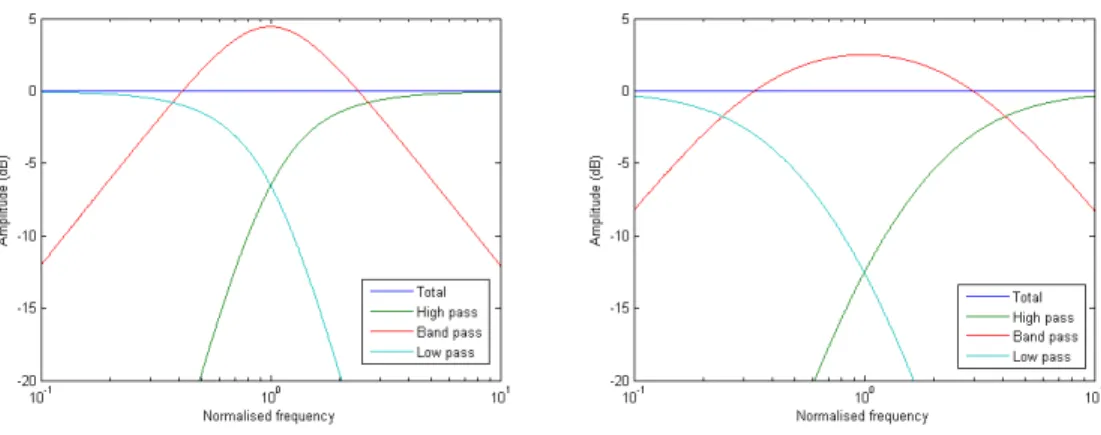
2.2.3. Symmetrical – three way

The equation can be split into three channels:

2 0 0 1 2 2 0 0 1 0 1 2 2 0 0 1 2 0 2 1 1 1 1 s s a H s s a s a H s s a s H LP BP HP + + = + + = + + =

The cut-off slope is ±12 dB/octave for the bass and treble channels and ±6 dB/octave for the midrange channel so the treble loudspeaker is protected but the midrange loudspeaker must cover a range of 6 octaves total. Coefficient a1 represents the quality

factor (Q = 1/ a1), thus defining the pulse response of the individual channels; the

resultant pulse response of the complete system is unity when the outputs are combined, assuming perfect addition of the channels.

(23)

At the crossover frequency, and assuming a1 = 2, we get: ° − ∠ = = − + = ° ∠ = − + = ° ∠ = − = − + − = 90 50 . 0 2 1 1 2 1 1 0 1 1 2 1 2 90 50 . 0 2 1 1 2 1 1 2 2 2 i i H i i H i i H LP BP HP

So, the low-pass and high-pass channels cancel at crossover and leaves the midrange to fill the gap. The design was originally proposed by Bang & Olufsen and labelled as the

Filler Driver system. The name indicates that the middle channel was not considered a conventional midrange channel but rather a phase correction of a two-way system.

Bass REB LB1 CT1 Treble RET LT1 CB1 CM1 Treble RET LM1

Figure 16 – Passive crossover network.

Two examples are shown, using Q = 1, which represents a 1 dB Chebychev filter characteristic of the second-order filter, and Q = 0.5, which represents the limit where the channels are unconditionally stable (real roots).

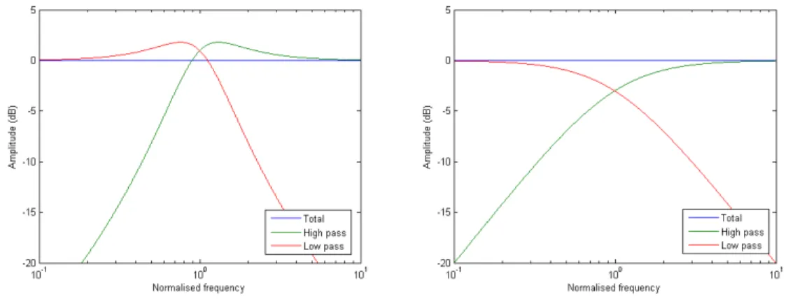
Figure 17 – Amplitude and phase response with a1 = 1.

The phase difference between the neighbour channels is 90° throughout frequency and 180° between the low-pass and high-pass channels.

(24)

Figure 18 – Amplitude and phase response with a1 = 2.

2.2.4. Steep cut-off – two way

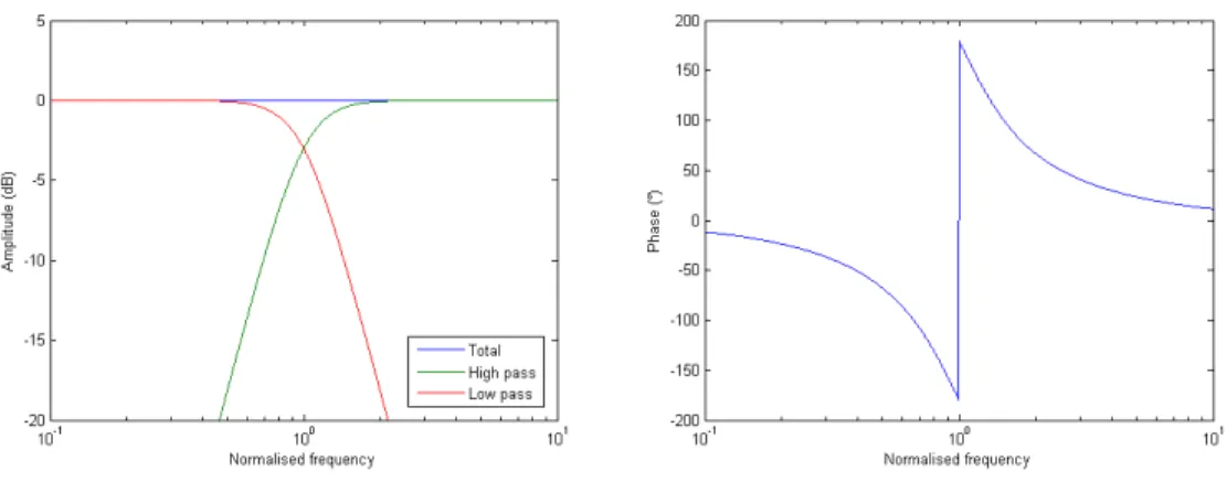
Maximum cut-off slope of both channels is obtained if the first-order term is removed from the nominator, resulting in a two-way crossover. The filter does not satisfy the requirement of unity transfer function since H2≠ 1 but it can realise an all-pass filter.

2 0 0 1 2 2 0 0 1 2 0 2 1 1 1 s s a H s s a s H LP HP + + = + + =

Determination of the coefficients assume modelling by a combination of two first-order Butterworth filters in cascade (the Linkwitz-Riley method). The nominator polynomial is not important for this evaluation, only the denominator polynomial is considered.

2 0 0 2 1 2 0 1 2 1 2 2 1 1 s s N s N H H_LP _LP + + =       + = =

By comparison, the coefficient is found to: 2

1= a

The transfer functions of the channels become:

2 0 2 0 2 2 0 2 2 1 2 1 1 o HP o LP s s s H and s s H + + = + + =

The resultant transfer function becomes:

2 0 2 0 2 2 1 1 o s s s H + + + =

At crossover is s0 = i so the nominator equates zero; i.e. the filter introduces a notch at

(25)

Bass REB LB1 CT1 Treble RET LT1 CB1

Figure 19 – Passive crossover network.

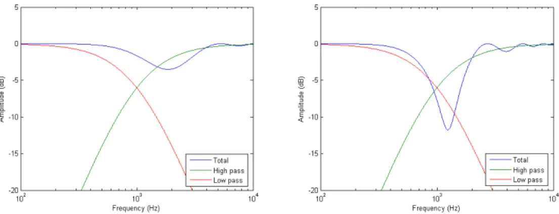
Figure 20 – Amplitude phase response with a1 = 2. The notch at crossover is due to the phase difference between the loudspeaker. The bass loudspeaker is –90° and the treble loudspeaker is 90°, i.e. 180° apart, so the outputs cancel.

A solution is to invert the polarity of one of the channels, often the treble loudspeaker, which restores the phase difference to 0°. The resultant transfer function becomes:

2 0 0 1 2 0 2 2 2 1 1 s s a s H H H _LP _HP + + − = − =

The resulting amplitude response is flat but the phase decreases gradually from 0° at low frequencies to –180° at high frequencies. This is a small price to pay for a filter with sufficient cut-off slope to reduce the bandwidth requirement to 1 octave outside cut-off and to protect the treble loudspeaker against low-frequency signals.

(26)

The introduction of a phase different from zero introduces a group delay, which is shown in Figure 22. Note that the group delay unit is calculated for a normalised filter corresponding to a cut-off frequency of 1 Hz. With a cut-off frequency of 1000 Hz the group delay scaling will be in milliseconds and not seconds.

Figure 22 – Group delay with a1 = 2 and inverted treble channel.

The filter is very popular due to the low component count of two components per channel and relative steep cut-off.

(27)

2.3. Third order

Ideal crossover networks of third order are problematic, as will be shown in this section. The problem being large phase difference between channels, which results in quite odd designs.

A third-order transfer function is defined from HN with N = 3: 3 0 2 0 2 0 1 3 0 2 0 2 0 1 3 1 1 s s a s a s s a s a H + + + + + + =

Determination of the coefficients assume modelling by a combination of a first-order filter and a second-order filter in cascade. The nominator polynomial is not important for this evaluation, only the denominator polynomial is considered.

(

)

(

)

3 0 2 0 0 2 1 2 0 2 1 2 1 3 1 1 1 1 1 s s c s c N N s cs N s N H H H_LP _LP _LP + + + + + = + + × + = × =

By comparison, the coefficients are found to:

c a c a + = + = 1 1 2 1

The value of c must be chosen for the use with all-pass filters. The phase difference between the channels is 270° at crossover (since i3 = –1), so the signals are added with a loss of 3 dB. The crossover filters should thus be –3 dB and since the first-order filter realises this, the second-order filter must be set to 0 dB at crossover so it requires c = 1 since c = 1/Q for the second-order filter defines the level at resonance (equal to Q).

2.3.1. Asymmetrical – two way

One obvious realisation of a two-way crossover network is to divide between the first-order and second-first-order terms:

3 0 2 0 2 0 1 2 0 2 0 1 3 3 0 2 0 2 0 1 3 0 3 1 1 1 s s a s a s a s a H s s a s a s H LP HP + + + + + = + + + =

A passive implementation is sensitive to loudspeaker impedance because of the series elements. The damping must be supplied by the load resistance, the loudspeaker, which is far from resistive if not compensated properly, so the passive crossover network requires impedance compensation of both branches.

(28)

At crossover, and assuming a1 = a2 = 2 for simplicity, we get: ° − ∠ = − − = + − + − = − − + − + = ° + ∠ = − = + − − = − − + − = 18 58 . 1 1 2 1 1 2 1 2 2 1 2 2 1 135 71 . 0 1 1 2 2 1 3 3 i i i i i i i H i i i i i i i H LP HP

So, the channels are 153° out of phase at crossover but the level is increased for the low-frequency channels to compensate for the loss and the channels add up to 0°. This is not a healthy way of designing a crossover network, the design should not be based upon subtraction of large figures; this will easily lead to problems.

Bass REB LB1 CT1 Treble RET LT RB1 CB RB2 LB2 CT2

Figure 23 – Passive crossover network.

An active filter realisation could use the following algorithm to extract the low-pass channel from the high-pass channel.

3

3 1 HP

LP H

H = −

The resulting amplitude response is shown below for two arbitrarily selected values of the coefficients a1 and a2.

Figure 24 – Amplitude response with a1 = a2 = 2 (left) and a1 = a2 = 3 (right).

The peaking becomes worse for smaller values and the slope becomes too soft for larger values of a1 and a2 so this is not a particularly valuable design. The high-pass filter

cut-off slope is 18 dB/octave, but the low-pass channel is only –6 dB/octave so the loudspeaker must be well-behaved three octaves above the cut-off frequency.

(29)

2.3.2. Symmetrical – two way

One obvious realisation of a two-way crossover network is to divide between the second-order and third-order terms:

3 0 2 0 2 0 1 0 1 3 3 0 2 0 2 0 1 3 0 2 0 2 3 1 1 1 s s a s a s a H s s a s a s s a H LP HP + + + + = + + + + =

Cut-off slope is ±12 dB for both channels and the filter is symmetrical for a1 = a2. At

crossover, and assuming a1 = a2 = 2 for simplicity, we get:

° − ∠ = − + − = + − + = − − + + = ° + ∠ = − + = + − − − = − − + − − = 72 58 . 1 1 2 1 1 2 1 2 2 1 2 1 72 58 . 1 1 2 1 2 2 2 1 2 3 3 i i i i i i i H i i i i i i i H LP HP

So, the channels are 144° out of phase at crossover but the level is increased for both channels to compensate for the loss and the channels add up to 0°. This is not a healthy way of designing a crossover network, the design should not be based upon subtraction of large figures; this will easily lead to problems.

A passive implementation is sensitive to loudspeaker impedance because of the series elements. The damping must be supplied by the load resistance, the loudspeaker, which is far from resistive if not compensated properly.

Bass REB LB1 CT1 Treble RET LT1 CB1 RB1 LB2 RB1 CT2

Figure 25 – Passive crossover network.

3

3 1 HP

LP H

H = −

The resulting amplitude response is shown below for two arbitrarily selected values of the coefficients a1 and a2. The cut-off slope is sufficient to reduce the loudspeaker

requirement to 2 octaves past the crossover frequency and using a value of a1 = a2

around 4 seems useful since the peaking is limited to around 1 dB for each channel, which could be expected to work in real life.

(30)

Figure 26 – Amplitude response with a1 = a2 = 2 (left) and a1 = a2 = 3.7 (right).

2.3.3. Symmetrical – three way

A symmetrical three-way crossover network can be build by using the middle two terms for the midrange loudspeaker:

3 0 2 0 2 0 1 3 3 0 2 0 2 0 1 2 0 2 0 1 3 3 0 2 0 2 0 1 3 0 3 1 1 1 1 s s a s a H s s a s a s a s a H s s a s a s H LP BP HP + + + = + + + + = + + + =

Cut-off slope is ±18 dB/octave for the bass and treble channels but only ±6 dB/octave for the midrange channel. The filter will be symmetrical for a1 = a2.

A passive implementation is not attractive but the active solution is straightforward, when the low-pass and high-pass channels have been constructed:

3 3

3 1 LP HP

BP H H

H = − −

The low-pass and high-pass channels can be constructed from standard third-order Butterworth filter blocks – but the design is quite tricky as the following analysis will show. Assume that the coefficients are a1 = a2 = 2, to simplify the analysis. The

following amplitudes and phases can then be found at the crossover frequency (s0 = i):

° − ∠ = − − = + − = − − + = ° ∠ = − − = + − − = − − + − = ° + ∠ = − = + − − = − − + − = 135 71 . 0 1 1 1 1 2 2 1 1 0 2 1 1 2 1 1 2 2 2 1 2 2 135 71 . 0 1 1 2 2 1 3 3 3 i i i i H i i i i i i i H i i i i i i i H LP BP HP

So, the low-pass and high-pass channels combine to –1 at crossover while the midrange channel is at 0°, which means that the two channels opposes the midrange channel. The midrange channel must be boosted to 2 in order for the sum of all channels to be unity.

(31)

Figure 27 - Amplitude response for the symmetrical third-order three-way crossover network with a1 = a2 = 2.5 (left) and a1 = a2 = 4 (right).

The conclusion is, that the design would do better without the midrange channel, and this is exactly the following crossover network to be analysed. This is at the end of the ideal filters with H = 1, since higher order filters includes too many terms; they are cumbersome to implement, especially with passive filters.

2.3.4. Steep cut-off – two way

In order to improve the cut-off slope of the low-pass channel one method is to remove the a1 and a2 coefficients of the nominator:

3 0 2 0 2 0 1 3 3 0 2 0 2 0 1 3 0 3 1 1 1 s s a s a H s s a s a s H LP HP + + + = + + + =

3

3 1 HP

LP H

H = −

Again, the passive filter must use impedance compensation of the loudspeakers.

Bass REB LB1 CT1 Treble RET LT1 CB1 LB2 CT2

Figure 28 – Passive crossover network.

The coefficients must be a1 = a2 = 2 for the all-pass filter and the result is shown in

Figure 29. The phase does not jump 360° at crossover; this is due to the MATLAB

(32)

Figure 29 - Amplitude and phase response with a1 = a2 = 2.

The introduction of a phase different from zero introduces a group delay shown in Figure 30. Note that the group delay unit is calculated for a normalised filter corresponding to a cut-off frequency of 1 Hz. With a cut-off frequency of 1000 Hz the group delay scaling will be in milliseconds and not seconds.

Figure 30 – Group delay with a1 = a2 = 2.

The filter includes two coefficients and its sensitivity to variations was analysed by scaling the coefficients by ±10 % with the result shown in Figure 31.

(33)

Figure 31 - Amplitude response for 10 % change of coefficients: a1 = 1.8, a2 = 2.2 (left) and a1 = 2.2, a2 = 1.8 (right).

The filter accept inversion of the treble loudspeaker.

Figure 32 - Amplitude and phase response with a1 = a2 = 2 and inverted treble.

The group delay is reduced in amplitude and becomes monotonically as result of the inversion, so although one may argument against the inversion, there could be an audible improvement by doing so.

(34)

2.4. Fourth order

Crossover networks of fourth-order are popular due to the steep cut-off slopes, which reduces the loudspeaker requirement to less than 2 octaves beyond the crossover frequency. However, a passive implementation is practical only for the all-pass filter, since component count would be too large with the three-way system.

A fourth-order transfer function is defined from HN with N = 4: 4 0 3 0 3 2 0 2 0 1 4 0 3 0 3 2 0 2 0 1 4 1 1 s s a s a s a s s a s a s a H + + + + + + + + =

2.4.1. Symmetrical – three way

A symmetrical three-way crossover network can be build using the middle term for the midrange loudspeaker. Coefficient a2 must be removed from the nominator.

4 0 3 0 3 2 0 2 0 1 0 1 4 4 0 3 0 3 2 0 2 0 1 2 0 2 4 4 0 3 0 3 2 0 2 0 1 4 0 3 0 3 4 1 1 1 1 s s a s a s a s a H s s a s a s a s a H s s a s a s a s s a H LP BP HP + + + + + = + + + + = + + + + + =

An active implementation could use:

4 4

4 1 LP HP

BP H H

H = − −

The low-pass and high-pass channels includes two terms each so they cannot be implemented using standard low-pass and high-pass filters but the circuitry is not too complex to be implemented using active filters. When build, the midrange channel is derived by subtracting the channels from the input signal.

Assume that the coefficients are a1 = 2, a2 = 3 and a3 = 2, to simplify the analysis. The

following amplitudes and phases can then be found at the crossover frequency (s0 = i):

° − ∠ = − + = + − − + + = ° ∠ = − − = + − − + − = ° ∠ = − − = + − − + + − = 243 2 . 2 1 2 1 1 2 3 2 1 2 1 0 0 . 3 1 3 1 2 3 2 1 3 243 2 . 2 1 2 1 1 2 3 2 1 1 2 3 3 3 i i i i H i i H i i i i H LP BP HP

So, the low-pass and high-pass channels are 486° out of phase (corresponds to 126°) and adds with some loss and the midrange channel adds the required signal. The channels are all at fairly high levels around crossover so this is a design, which is based upon subtraction of large figures – it should be avoided.

(35)

Figure 34 – Amplitude and phase with a1 = 2, a2 = 3, a3 = 2.

2.4.2. Steep cut-off – two way

The terms with a1, a2 and a3 are removed from the nominator resulting in a two-way

crossover with maximum cut-off slope within both channels. The filter does not satisfy the requirement of unity transfer function.

4 0 3 0 3 2 0 2 0 1 4 4 0 3 0 3 2 0 2 0 1 4 0 4 1 1 1 s s a s a s a H s s a s a s a s H LP HP + + + + = + + + + =

Determination of the coefficients assume modelling by a combination of two second-order Butterworth filters in cascade (the Linkwitz-Riley method). The nominator polynomial is not important for this evaluation, only the denominator is considered.

(

)

4 0 3 0 2 0 2 0 2 1 2 0 0 2 2 0 0 1 2 2 4 2 2 2 1 2 , 1 1 s cs s c cs N N c where s cs N s cs N H H H_LP _LP _LP + + + + + = = + + × + + = × =

By comparison, the coefficients are found to:

83 . 2 2 00 . 4 2 83 . 2 2 3 2 2 1 = = = + = = = c a c a c a

A passive implementation is at the limit of what can (or should) be done but the network is straight forward from a theoretical point of view. It is a requirement that the loudspeakers are impedance compensated.

(36)

Bass REB LB1 CT1 Treble RET LT1 CB1 LB2 CT2 CB2 LT2

Figure 35 – Passive crossover network.

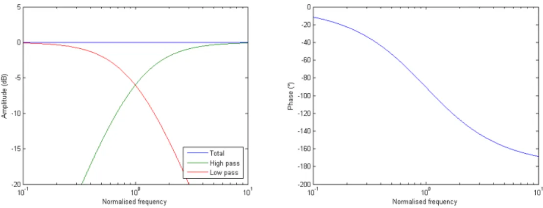
The result is shown in Figure 36. The phase difference between the channels are 360° at crossover so the signals are added without loss.

Figure 36 – Amplitude and phase response with a1 = a3 = 2.83, a2 = 4.00.

(37)

2.5. Passive network

A passive network is best suited for low order crossover networks and can be build as shown in Figure 38, where Z1, Z2, etc. are impedances, which may consist of resistors,

inductors and capacitors or even combinations hereof. The number of branches is defined by the filter order; a first order crossover network would consist of Z1 only.

RE Z3

Z2 Z1

Figure 38 – Conventional ladder-network for a passive crossover. The impedances can be any of resistor, inductor or capacitor.

The transfer function of the filter can be derived from inspection of the circuitry. The below collection of crossover network transfer functions is limited to third order since higher order networks become more involved and are of little practical use. Higher order filters should preferably be build using active circuitry.

2.5.1. First order

This consists only of Z1 so Z2 not used and Z3 is a short circuit. The filter is a voltage

divider between the series element Z1 and the loudspeaker, represented by the DC voice

coil resistance RE. The transfer function for the first order network is:

E E R Z R H + = 1 1

To introduce real components, the impedance must be substituted by an inductor or a capacitor. The impedance of the inductor and capacitor is defined as:

sC Z sL Z C L 1 = =

Using an inductor for Z1 the result is a low-pass filter:

L R where s R sL R sL R H E E E E LP = ₊ = + = + = ₀ 0 1 , 1 1 1 1 _ω