REWIRE: An Optimization-based Framework for
Data Center Network Design
Andrew R. Curtis, Tommy Carpenter, Mustafa Elsheikh, Alejandro L´opez-Ortiz and S. Keshav
Cheriton School of Computer ScienceUniversity of Waterloo
University of Waterloo Tech Report CS-2011-21
Abstract—Despite the many proposals for data center network (DCN) architectures, designing a DCN remains challenging. DCN design is especially difficult when expanding an existing network, because traditional DCN design places strict constraints on the topology (e.g., a fat-tree). Recent advances in routing protocols allow data center servers to fully utilize arbitrary networks, so there is no need to require restricted, regular topologies in the data center. Therefore, we propose a data center network design framework, REWIRE, that designs networks using a local search-based algorithm. Our algorithm finds a network with maximal bisection bandwidth and minimal end-to-end latency while meeting user-defined constraints and accurately modeling the predicted cost of the network. We evaluate REWIRE on a wide range of inputs and find that it significantly outperforms previous solutions—its network designs have up to 100–500% more bisection bandwidth and less end-to-end network latency than best-practice data center networks.
I. INTRODUCTION
Organizations have deployed a considerable amount of data center infrastructure in recent years, and much of this has been from the expansion and upgrading of existing facilities. For example, a recent survey found that nearly 2/3s of data center operators in the U.S. have added data center capacity in the past 12–24 months and 36% plan on adding capacity in 2011 [17]. Most existing DCNs are small- to medium-sized1 and use a vendor-defined network architecture. These architectures, such as Cisco’s [11], arrange the topology as a 1+1 redundant tree. Doing so results in underprovisioned networks, for example, Microsoft researchers [20] found links as much as 1:240 oversubscribed in their data centers. Such heavily oversubscribed networks constrain server utilization because they limitagility—the ability to assign any server to any service—and they lack sufficient bisection bandwidth for modern distributed applications such as MapReduce, Dryad [30], partition-aggregate applications [3], and scientific com-puting.
Despite this, operators have little guidance when planning and executing a data center expansion or upgrade. Designing a new or updated network is a challenging optimization problem that needs to optimize multiple objectives while meeting many
175% of survey respondents in the US have data centers with
power load of less than 2.0 MW [17], which implies they run fewer
than 4000 servers if each server draws 500 W (including the power to cool it).
constraints. Most physical data centers designs are unique, so expansions and upgrades must be custom designed for each data center (see, e.g., industry white papers [51]). The optimization challenge is to maximize network performance (which includes bisection bandwidth, end-to-end latency and reliability) while minimizing costs and satisfying a large number of constraints.
We propose REWIRE, an algorithm to design new, upgraded and expanded DCNs. Unlike previous solutions, REWIRE does not place strict restrictions on the space of topologies considered. Instead, it maximizes bisection bandwidth and minimizes end-to-end latency of its network designs by search-ing the space of all networks that are feasible under a user-specified data center model.
In particular, our main contributions are:
1) We propose a model to characterize the data center network design problem.
2) We introduce a data center design algorithm REWIRE that designs greenfield, upgraded or expanded networks for a user-specified data center model using local search. 3) We evaluate REWIRE by comparing it to several other
methods of constructing data center networks.
To find an optimized network, REWIRE uses a local search, so it evaluates many candidate network designs. However, computing the performance of a network involves determining its bisection bandwidth. We are not aware of any previous polynomial-time algorithm to compute the bisection band-width of an arbitrary network; however, we show that it can be found by solving a linear program (LP) given by Lakshman et al. to find an optimaloblivious, or static, routing. Unfortu-nately, this LP hasO(n4)variables and constraints, where n
is the number of switches in the network, so it is expensive to find even for small networks. To speed this process, we implement an(1+)-approximation algorithm to compute this LP [36]. We further speed the run-time of this approxima-tion algorithm implementing its bottleneck operaapproxima-tion—an all-pairs shortest-path computation—on the GPU using NVIDIA’s CUDA framework [42]. Our implementation is 2–23x faster than a high-performance CPU implementation. Additionally, we utilize a heuristic based on the spectral gap of a graph, which is the difference between the smallest two eigenvalues of a graph’s adjacency matrix. We find that the spectral gap of
a graph is a useful heuristic for candidate selection, especially when designing greenfield (newly constructed) DCNs.
The closest related work to REWIRE is LEGUP [14], another framework to design DCN upgrades and expansions. However, their approach imposes a heterogeneous Clos topol-ogy on the updated network, and also requires a Clos network as input. We seek a general solution—one that accepts any network as input and returns arbitrary topologies.
We find that moving to an arbitrary DCN topology has significant performance benefits. When designing greenfield (i.e., new) data center networks, REWIRE’s networks have at least 500% bisection bandwidth than a fat-tree constructed with the same budget. When upgrading or expanding an exist-ing network, REWIRE achieves similar performance gains and beats a greedy algorithm as well. Moving to an arbitrary DCN topology does create operational and management concerns since most DCN architectures are topology-dependant. We address these issues in Sec. V.
II. DEFINING THEPROBLEM
Designing a data center network is a major undertaking. The solution space is massive due to the huge number of variables and an ideal network maximizes many objectives simultaneously. Our goal is to automate the task of designing the best network possible given a user’s budget and a model of their data center. We primarily target small- to mid-sized data centers because (1) it is expensive for small data center operators to hire consultants to re-design their network (whereas large data center operators may be able to perform this task in-house) and (2) most data centers have fewer than 4000 servers [17]. Ideally, a user of our system need only hire staff to re-wire the DCN according to the system’s output. In the remainder of this section, we describe the data center environment and state our assumptions.
A. Network design and assumptions
We now describe DCN workloads and their impact on topology design.
Workload assumptions:from available DCN measurement studies [5], [31], we know that DCN workloads exhibit a high degree of variance, and therefore must be provisioned accordingly. In a 24 hour time period, there can be an order of magnitude difference between the peak and minimum load in the DCN [27]. The network needs enough capacity to account for this daily fluctuation, and it should account for future demand. DCN traffic is also unpredictable over short periods. Studies indicate that DCNs exhibit highly variable traffic [31], [6], [20], [5], that is, the traffic matrix (TM) in a DCN shifts frequently and its overall volume (i.e., the sum of its entries) changes dramatically in short periods.
Because of the variability in DCN traffic, we assume that an ideal DCN can feasibly route all hose traffic matrices, which are the traffic matrices where a node i sends or receives at mostr(i)traffic at once. Typicallyr(i)is equal to the sum of NIC uplinks ati. We denote the polyhedron of hose TMs valid for nodes1, . . . , nbyT(r(1), . . . , r(n)). The switching fabric
is never a bottleneck in a network that can feasibly route all hose TMs—instead, flows are limited only by contention for bandwidth at end-host NICs.
Topology design:greenfield data centers are typically built with a highly regular topology. Most DCNs, especially small-to medium-sized DCNs, are built following vendor guidelines, which generally arrange the network as a 3-level, 1+1 redun-dant tree topology. In this topology, each rack contains 20–80 servers that connect to a top-of-rack (ToR) switch. A typical ToR switch has 48 1Gbps and up to four 10Gbps ports. These ToR switches are the leaves of the multi-rooted switching tree. This tree usually has three levels: the ToR switches connect to a level of aggregation switches, which connect to a core level made up of either switches or routers. The core switches are typically connected to a pair of edge routers which connect the data center to the internet.
Theoretical topology constructions date back to telephone switching networks, when the goal was to interconnect cir-cuits. A variety of topology constructions have been proposed over the years to interconnect hundreds of thousands of servers, for example, [12], [14], [4], [47], [34], [1], [52], [23], [22]. The general theme of work in this area is to scale-out, that is, these topologies use multiple commodity switches in place of a single high-end switch.
Cost-effective topology design is important to data center operation, because providing enough bisection bandwidth is crucial to reducing the overall cost of operating a data center because it allows for higher server utilization. Servers account for over 45–60% of the cost of building a large-scale data center [21] and server utilization is generally 10–20% with an average utilization of 30% being very good [24]. Networks with too little bisection bandwidth cannot allocate servers to jobs timely enough to improve utilization further [20]. B. Switches, links and end-hosts
Most data centers today run on commodity off the shelf (COTS) servers and switches. Using COTS equipment reduces costs, so we assume the network will be composed of COTS switches. There are many such switches to choose from, each with different features. As such, we allow users to define the specifications of switches available to add to their data center. For example, we enable the user to input details about line cards available for a particular switch type. Also, users can specify a processing delay for each switch, which indicates the amount of time it takes the switch to forward a packet when it has no other load.
Links can be optical or copper and can use incompatible connector types. Currently, we do not model the difference in link medium or connectors; instead, we assume that all 1Gb ports use the same connector and all 10Gb ports use the same connector. Copper links also pose a problem because they are limited to runs of less than 5–10m when operating at 10Gbps [39]. It would not be difficult to check for link medium and connector types; however, we do not do so currently.
We assume that the data center operator has full control over end-hosts. That is, they can install custom multipath routing
protocols, like Multipath TCP [46] and SPAIN [38], on all end-hosts. This assumption does not hold in cloud settings, where customers can run their own OS installations. Here, the cloud provider could release a set of OS images that have the required end-host modifications installed.
C. Physical design and constraints
There are many physical restrictions placed on the design of a DCN. We now discuss the constraints that make adding equipment to a data center challenging.
Most data centers house equipment in large metal racks, and a standard rack is 0.6 m wide, 2 m tall by 1 m deep and is partitioned into 42 rack units (denoted by U). A typical server occupies 1–2U and switches occupy 1U for a top-of-rack switch up to 21U for large aggregation and core switches. We assume that all equipment must be placed in a rack, and that the racks are positioned alongside each other so they form rows.
Data center power delivery systems are complex and expen-sive. Power to servers is deliverd by power distribution units (PDUs), which then power servers and network equipment. A typical PDU handles 75–225 kW of load [27]. We model a data center’s power system by its PDUs, that is, if any PDU has enough capacity to power a device, then it can be added to the data center floor.
Data center equipment creates a significant amount of heat, which must be dissipated by a cooling system. For every watt spent powering IT gear, it takes 1 watt to cool it in the average data center [19]. Therefore, cooling is a constrained resource, so we assume that each rack has a limit on the amount of heat its contents may generate.
Cabling also has physical limitations because cables adds weight to and take up space in plenums, which are trays that carry cables between rows. Modeling these limitations is challenging as Mudigonda et al. describe [39]. At this point, we do not model physical layout of cabling; however, REWIRE’s design supports adding these constraints in the future.
D. DCN performance: what’s important to applications? The two most important characteristics of DCN perfor-mance are high bisection bandwidth and low latency. Bisection bandwidth is especially important, because when the network has enough bisection bandwidth, all servers can fully utilize their NICs no matter where they are sending data to or what other servers on the network are doing. This is ideal— end-hosts are the limiting factor in such a network, not the switching fabric. Spare bisection bandwidth also keeps end-to-end latencies across the network low, because links will be lightly loaded, and hence queuing delays will be minimal. Minimal latency is important for interactive data center jobs, such as search and other partition-aggregate jobs, where up to hundreds of worker servers perform jobs for a service. The results of these jobs are aggregated by a master server. Latency is critical for this type of service because responses
from workers that do not respond by a deadline (usually 10– 100ms) are not included in the final results, lowering result quality and potentially reducing revenue [3].
E. Cost model
Estimating the cost of building a DCN design is very difficult. There are two major obstacles to accurately pricing a DCN design: (1) it is hard to get prices of switches— street prices are often a fraction of retail prices and can be difficult to obtain. Vendors offer discounts for bulk purchases, so the price of a switch often decreases as more of its type are purchased. And, (2) it is difficult to estimate the cost of cabling a DCN. Cables that are too long incur installation costs because the contractor has to hide cabling. Bundling cables together in long runs also reduces the cost of wiring long-distance links [45], [39], though we are not aware of any algorithms to compute the cost of such a wiring. Finally, it may be more expensive to wire irregular topologies compared to regular topologies; however, we do not have any data on this, so we bill per link, regardless of the topology structure. For tractability reasons, we assume fixed prices for switches. That is, the switch prices specified by the user should be an estimate of how much the switch will cost even if just a single switch of its type is purchased. For cabling, we divide cable lengths into different categories (e.g., short, medium and long) and charge for a cable based on its length category.
III. REWIRE ALGORITHM
We now describe the operation of REWIRE, starting by formally stating the problem it solves. It performslocal search, so it starts with a candidate solution, which is a network design that does not violate any constraints. It explores the search space of all candidate solutions by moving from one candidate to another by modifying local properties of the solution until a near-optimal solution is found. This local search only optimizes the network’s wiring—it does not add switches to the network. Therefore, we end this section by describing how to extend our approach to add new switches to the network as well.
A. Optimization problem formulation
REWIRE’s goal is to find a network with maximal perfor-mance, subject to numerous user-specified constraints.
1) Optimization objective: REWIRE designs networks to jointly maximize bisection bandwidth while minimizing the worst-case latency between ToR switches, that is, given the fixed scalarsαandβ, our objective function is:
maximize : α·bw(G)−β·latency(G)
wherebw(G)andlatency(G)are defined as follows: • Bisection bandwidth: denoted bw(G), depends on the
rate, r(i), of a node i, which we define as the peak amount of traffic v can initiate or receive at once. For example, a servervwith a 1Gbps NIC hasr(v) =1Gbps. For simplification, we aggregate the bandwidth from all servers attached to a ToR switchsat that switch, that is,
we let the rater(i)of a ToR switch ibe the sum of the rates of servers directly connected to the switch (e.g., a ToR switch connected to 40 servers, each with a 1Gbps NIC, has a rate of 40Gbps). The bisection bandwidth of a networkGis then: bw(G) = min S⊆V P e∈δ(S)w(e) min{P i∈Sr(v), P i∈Sr(v)}
where δ(S) is the set of edges with one endpoint in S
and another in S=V −S.
• Worst-case latency:is defined as the worst-case shortest-path latency between any pair of ToR switches in the network, where the latency of a path is the sum of queuing, processing, and transmission delays of switches on the path. We assume that the queuing delay at any port in the network is constant because we have no knowledge of network congestion while designing the network. Both of these metrics have been considered in the design of DCN topologies, e.g., [20], [39]. However, as far as we know, no previous algorithms could compute the bisection bandwidth of an arbitrary network in polynomial-time. Therefore, we propose such an algorithm by combining previous theoretical results in Sec. III-B1.
Previous work has modeled latency by the worst-case hop-count in the network—this is the network’s diameter. Our definition of latency takes into account the speed of links on the path and the processing time at switches. Taking into account processing time at switches is important because unoptimized switches can impose an order of magnitude more processing delay than switches optimized to minimize latency. Our definition of network latency is more difficult to compute than a definition based on hop-count, because the worst-case hop-count can be found in linear-time using breadth-first search, whereas our definition requires computing the full shortest-path tree of a network.
2) User-specified constraints: REWIRE incorporates a wide range of constraints into its optimization procedure. These are provided by the user, and are:
• Budget constraint. This is the maximum amount of cash the user is willing to spend on the network.
• Existing network topology and specifications.To perform an upgrade or expansion, we need the existing topology. If designing a greenfield network, then REWIRE needs a set of ToR switches given as the existing network because our current design does not attach servers to ToR switches. This input needs to include specifications for all network devices. For switches this includes their neighbors in the network and relevant details such as the number of free ports of each link rate. Our implemen-tation does not support different link types (e.g., copper vs. optical links); however, it would be easy to extend it so that links include the type of connectors on the ends. • Available switch prices and specifications (optional). If one would like to add new switches to the network, REWIRE needs as input the prices and specifications of a few switches available on the market. Specifications
include number and speeds of ports, peak power con-sumption, thermal output and the number of rack slots the switch occupies.
• Link prices and specifications. We need a price estimate for labor and parts for each link length category. • Data center model (optional).Consists of the following:
– Physical layout of racks;
– Description of each rack’s contents (e.g. switches, servers, PDUs, number of free slots);
– Per rack heat constraints; and/or – Per rack power constraints.
The data center model places constraints on individual racks. REWIRE uses these constraints to, for example, restrict the placement of new switches to racks with enough free slots.
• Reliability requirements (optional). This places a con-straint on the number of links in the min-cut of the network. That is, this is the minimum number of link removals necessary to partition the network into two connected components.
B. Local Search Approach
REWIRE uses simulated annealing (SA) [35] to search through candidate solutions. Our algorithm contains:
1) A finite spaceS of all network configurations that obey the hose, port, and budget constraints.
2) A constantIrepresenting the number of inner Metropo-lis iterations to be preformed (explained below). As
I → ∞, SA finds a guaranteed optimal solution, but the algorithm runtime is unfeasible for very large values of I [7]. We set I to 1000.
3) A real valued energy function E(s) defined ∀s ∈ S;
E(s)= −α∗bw(s) +β∗latency(s).
4) A set N(s) defined ∀s ∈ S—the set of all connected graphs with one link added or removed froms. 5) An initial temperature TST ART found using [35]. 6) A decreasing function T(k) : Z+ → R called the
cooling schedule, where T(k) is the temperature dur-ing the kth set of I Metropolis iterations. We chose
T(k) = TST ART ∗0.93k, but note there is extensive
theory behind choosing cooling schedules [41], [53]. 7) An initial state s0∈S—the input network.
We first note ifs0 is a permutation ofsfound by adding a link tos, E(s0)≤E(s), but ifs0 is a permutation found by subtracting a link, E(s0)≥E(s).
The goal of SA is to find the network that minimizes
E. We perform I Metropolis iterations K times as follows, starting at TST ART. At each iteration, we choose random i, j ∈ N, R ∈ {0,1} to generate a state s0 ∈ N(s). If
R = 1, we attempt to generate s0 by adding a 10Gbps link betweeni, jinssubject to the port and budget constraints. If this addition fails, we attempt to add a 1Gbps link. If either addition is successful, the move is accepted and otherwise rejected. If R = 0, we generate s0 by attempting to subtract a link of random speed between i, j (if one exists), subject
to the connectivity constraint. If the subtract fails we reject the move. Otherwise, if E(s0) =E(s), the move is accepted unconditionally. If E(s0)> E(s) the move is accepted with probability e−(E(s
0)−E(s)
T , known as the Metropolis criterion. SA avoids getting caught in local maxima by sometimes taking suboptimal moves. The Metropolis criterion controls this risk as a function of temperature: the limit of the criterion is 1 as
t → ∞ and 0 as T → 0. When T is high bad moves are likely to be accepted, but whenT is close to 0, bad moves are accepted with very low probability.
AfterIMetropolis iterations are preformed, the temperature is decreased according to the cooling schedule. The process is repeated K times, where K is the smallest integer such that
T(k)< .05.
1) Evaluating a candidate solution: To compute the per-formance of a candidate solution, we must compute bisection bandwidth and the diameter of the network.
Bisection bandwidth: recall that bisection bandwidth is defined on the minimal cut of all cuts of a graph. This is too expensive to compute directly on arbitrary graphs because a graph can have exponentially many cuts. However, we can compute the bisection bandwidth of an arbitrary graph by computing a two-phase routing for the network.
Two-phase routing, proposed by Lakshman et al. [36], is oblivious, meaning that it finds a static routing that minimizes the max link utilization for any traffic matrix in a polyhedron of traffic matrices. Two-phase routing divides routing into two phases. During phase one, each node forwards an αi fraction of its ingress traffic to nodei. During stage two, nodes forward traffic they received during phase one on to its final destination. We say that α1, . . . , αn are the load-balancing parameters of
a graph G = (V, E). The optimal values of the αi values depends onGand the set of hose TMsT(r(1), . . . , r(n))for
V = 1, . . . , n.
Before describing how to compute a two-phase routing, we show that finding the load-balancing parameters of a network gives use the network’s bisection bandwidth. We denote a cut
of Gby(S, S), whereS andS are connected components of
G andS =V −S. Letc(S, S)be the capacity of all edges with one endpoint in S and the other in S. The following theorem shows the desired result—that we can compute the bisection bandwidth of a graph from α1, . . . , αn.
Theorem 1 ( [16] ): A network G = (V, E) with node ratesr(1), . . . , r(n)and load balancing parametersα1, . . . , αn
can feasibly route all hose TMsT(r(1), . . . , r(n))using multi-path VLB routing if and only if, for all cuts (S, S)of G,
c(S, S)≥X i∈S αi· X i∈S r(i) +X i∈S αi· X i∈S r(i) whereS=V −S.
This theorem shows that a multi-commodity flow version of the famous max-flow, min-cut theorem holds for networks using two-phase routing under the hose model.
We now show how computeα1, . . . , αn using the results of
Lakshman et al., who proved that the αi values can be found
with linear programming (LP) [36]. Before presenting their LP, we need to introduce some notation. Let f be anetwork flow in the optimization sense. We use fk to denote flow k
wheres(k)and is the origin andt(k)is the destination of the flow. Then let fk(i, j)be the amount of flow placed on edge
(i, j) by flow fk. We denote the outgoing edges from node
i by δ+(i) its incoming edges by δ−(i). The capacity of an
edge(i, j)is denoted byc(i, j).
Optimal two-phase routing LP:
min µ Subject to: X w∈δ−(y) fk(w, y) = X z∈δ+(y) fk(y, z) ∀y 6=s(k), t(k) ∀k (1) K X k=1 fk(i, j)≤µ·c(i, j) (2) X j∈δ+(i)
fk(i, j) =αs(k)r(i) +αt(k)r(i) (3)
i=s(k),∀k
X
i
αi= 1 (4)
This LP can be computed in polynomial-time using an LP solver; however, it is computationally expensive because it has
O(n4) constraints andO(n4)variables. In our initial testing, we found that computing this LP for a network with 200 nodes and 400 (directed) edges needs more than 22GB of memory using IBM’s CPLEX solver [29]. Even with only 50 node networks, this LP takes up to several seconds to compute. REWIRE’s local search approach needs to evaluate thousands of candidate solutions; therefore, this LP is not fast enough for our purposes.
To solve these issues, we implemented an approximation algorithm by Lakshman et al. [36] to computeα1, . . . , αn in
polynomial-time. This algorithm finds a solution guaranteed to be within an(1 +)factor of optimal. The algorithm works by augmenting a node i’s value of αi iteratively. At each
iteration, the algorithm computes a weightw(e)for each edge
e ∈ E and then pushes flow to i along the shortest-paths toi based on these weights. The bottleneck operation in this algorithm is computing the shortest-path from each node to each other node given the weightsw(e). This operation needs to perform an all-pairs shortest-path (APSP) computation. The best running time we are aware of for an APSP algorithm is O(n3) (deterministic) [13] and O(n2)(probabilistic) [44].
Because this operation is the bottleneck, we implemented an APSP solver on a graphics processing unit (GPU). Used this way, the GPU is a powerful, inexpensive co-processor with hundreds of cores. Details of our GPU implementation of APSP are found in Appendix A.
Latency: we find latency(G) by computing APSP on the network, where each edge weight represents the expected
time to forward packets on that link. To estimate this, we set the weight w(i, j) of an edge (i, j) to be the sum of queuing delays, forwarding time and processing delay at
(i, j)’s endpoints. The processing delay of each switch is
specified by the user. We assume that the forwarding time is 1500 Bytes divided by the link rate (1 or 10Gbps) and that the queuing delays are constant for all ports. Our assumption of uniform queuing delays is not realistic but necessary; since we assume no knowledge of the network load, we cannot accurately determine queuing delays.
Therefore, we compute the diameter of a candidate solution by solving APSPs with these link weights. As discussed above, this is a computationally expensive process, so we use our GPU-based APSP solver (described in Appendix A) for this computation.
2) Candidate selection: Our simulated annealing approach is guaranteed to find a globally optimal solution, if let run for long enough. However, given the huge search space we explore, this could take too long, especially when many links need to be added to a network. Therefore, we added the ability to seed REWIRE’s simulated annealing procedure with a candidate solution. To find a seed candidate, we use a heuristic based on the spectral capof a graph.
Before we define the spectral gap of a graph, we need to introduce a few terms. The Laplacian of G= (V, E) is the matrix: L(i, j) = 1 ifi=j andd(i)6= 0, −√ 1
d(i)d(j) ifi andj are adjacent,
0 otherwise.
The eigenvalues ofLare said to the bespectrumofG, and we denote them by λ0 ≤ · · · ≤ λn−1. It can be shown that λ0 = 0 (see, e.g., [10] for a proof). We say that λ1 is the
spectral gapof G.
Intuitively, a graph with a “large” spectral gap will be regular (we omit a precise definition of large here—see any text book for details [10]), and the lengths of all shortest-paths betweeen node pairs are expected to be similar. Spectral gap has been used as a metric in network design before (e.g., [18], [49]) due to the nice properties of graphs with large spectral gaps. As an example, the following lemma shows that the spectral gap correlates with the diameter of a graph.
Lemma 1: LetG be a graph with diamterD ≥4, and let
K denote the maximum degree of any vertex of G. Then
λ1≤1−2 √ k−1 k (1− 2 D) + 2 D
That is, a graph with a large spectral gap has a low diameter. Therefore, we modified REWIRE so that it optionally performs a two stage simulated annealing procedure. In stage 1, its objective function is to maximize the spectral gap. The result from stage 1 is used to seed stage 2, where its objective function is to maximize bisection bandwidth and minimize latency. This way, stage 2 starts with a good solution and can converge quicker. When this two stage procedure is used, we say REWIRE is in hotstart mode.
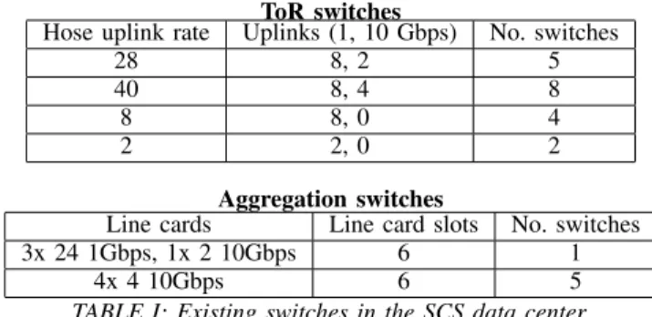
ToR switches
Hose uplink rate Uplinks (1, 10 Gbps) No. switches
28 8, 2 5
40 8, 4 8
8 8, 0 4
2 2, 0 2
Aggregation switches
Line cards Line card slots No. switches
3x 24 1Gbps, 1x 2 10Gbps 6 1
4x 4 10Gbps 6 5
TABLE I: Existing switches in the SCS data center.
Note that a network with a maximal spectral gap of all candidate solutions does not necessarily mean that the network will also have high bisection bandwidth. The spectral gap metric does not take the hose constraints into account, so it is not directly optimizing for bisection bandwidth. Instead, it creates networks that are well-connected, which tend to have high bisection bandwidth (see, e.g., [16] for details), but that is not necessarily the case, especially for heterogeneous networks.
C. Adding switches to the network
REWIRE’s simulated annealing procedure does not consider adding new switches to the network—it only optimizes the wiring of a given set of switches. To find network designs with new switches, we run REWIRE on the input network plus a set of new switches that are not attached to any other switch. REWIRE attaches the new switches to the existing network randomly, and then begins its simulated annealing procedure. While simple, this approach does not scale well. If a user has input specifications forknew switch types, then we need to run REWIREk!times to consider all possible combinations of switch types. We believe this could be improved by applying heuristics to select a set of new switches; however, we leave investigation of such heuristics to future work.
IV. EVALUATION
We now present our evaluation of REWIRE. First, we describe the inputs we use in our experiments, and then we the approaches we compare REWIRE to. Finally, we present our results using REWIRE to design greenfield, upgraded and expanded networks.
A. Inputs
1) Existing networks: To evaluate REWIRE’s ability to design upgrades and expansions of existing networks, we use the following network as inputs to REWIRE:
• The University of Waterloo’s School of Computer Sci-ence machine room network (denoted by SCS network), which has 19 ToR, 2 aggregation and 2 core routers. Each ToR connects to a single aggregation switch with a 1 or 10Gbps link and both aggregation switches connect to both core switches with 10Gbps links. The network is composed of a heterogeneous set of switches described in TableI.
To predict the cost of a network design, REWIRE needs the distance between each ToR switch pair. We do not have this data for the SCS network. Therefore, we label each switch with a unique label from 1, . . . , n. The distance between switches
i and j is then |i−j|. The distance from i to the nearest 25% of switches is categorized as “short”, the distance to the next 50% is “medium” and then distance to the final 25% is “long”. We use these distance categories to estimate the price of adding a link between two switches.
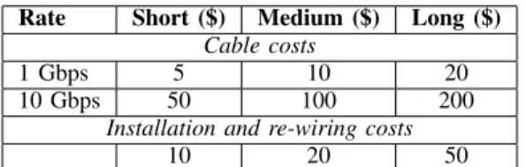
2) Switches and cabling: We separate the costs of adding a cable into the cost of the cable itself and the cost to install it. Mudigonda et al. report [39] that list prices for 10Gb cables are between $45–95 for 1m cables and $100–400 for 10m cables depending on the type of cable (copper or optical and its connector types). Optical cables are more expensive than copper cables, but they are available in longer lengths. To obtain a reasonable estimate of cabling costs without creating too much complexity, we divide cable runs into three groups: short, medium and long lengths. The costs we use are shown in Table II. We also charge an installation fee for each length group (also shown in the table). Whenever an existing cable is moved, we charge the appropriate installation fee given the cable’s length.
Rate Short ($) Medium ($) Long ($)
Cable costs
1 Gbps 5 10 20
10 Gbps 50 100 200
Installation and re-wiring costs
10 20 50
TABLE II: Prices of cables and the cost to install or move cables.
TableIIIshows the costs we assume to buy various switches. Ports Watts Price ($)
24 1Gbps 100 250
48 1Gbps 150 1,500
48 1Gbps, 4 10Gbps 235 5,000
24 10Gbps 300 6,000
48 10Gbps 600 10,000
TABLE III: Switches used as input in our evaluation. Prices are representative of street prices and power draw estimates are based on a typical switch of the type according to manufacturers’ estimates.
B. Comparison approaches
We compare REWIRE against the following DCN design solutions.
Fat-tree: was proposed by Leiserson [37] and is a k -ary multi-rooted tree. We assume a 3-level fat-tree topology and that all switches in the network must be homogeneous. Building an optimal fat-tree for a set of servers given switch specifications is NP-hard [39], so we upper bound the perfor-mance that a fat-tree network with a specified budget could achieve. To do this, compute the number of ports the fat-tree needs, and bound the cost of switches by the min-cost port of a given rate (e.g., a 1Gb port costs at least $250/24 and a 10Gb port costs at least $10K/48). To estimate the cost of cabling, we assume that server to ToR links are free, and that ToR to
aggregation switches are medium length and aggregation to core links are long length.
Greedy algorithm: we implemented a greedy heuristic to determine if REWIRE’s more sophisticated local search ap-proach is necessary. The algorithm iterates over all pairs of switches as follows. First, it computes the change in agility and latency that would result from adding a 1Gbps and 10Gbps between every pair of switches and stores the result. At the end of each iteration, the algorithm adds the link that increases the network’s performance the most. If no link changes the agility or latency during an iteration then a random link is added. This iteration continues until the budget is exhausted or no links can be added because all ports are full. Note that this algorithm does not rewire the initial input—it only adds links to the network until the budget is exhausted. This algorithm performs
O(n2)bisection bandwidth computations at each iteration, and hence does not scale to graphs with more than ∼40 nodes. Therefore, we do not compare against the greedy algorithm for any network with more than 40 nodes.
Random graph:Singla et al. proposed a DCN architecture based on random graph topologies [48]. Random graphs have nice connectivity properties, and they showed that it’s less expensive to build a random graph than a fat-tree much of the time. To estimate the performance a random graph can achieve with a specified budget, we determine the expect radix of each ToR switch given number of links one can install with the budget. Then, we compute the expected bisection bandwidth and diameter of the network following Singla et al.’s approach. REWIRE can operate in several different modes. These are: • Spectral gap mode:sets REWIRE to maximize the
spec-tral gap of the solution as described in Sec.III-B2. • CPLEX or approximation:sets the method REWIRE uses
to compute the bisection bandwidth of a network. In CPLEX mode, REWIRE uses IBM’s CPLEX solver [29] to compute the bisection bandwidth exactly; whereas in approximation mode, REWIRE finds the bisection band-width of a candidate solution using the FPTAS described in Sec.III-B1.
• Hotstart:this mode finds a candidate solution in spectral gap mode, which is used as a seed solution to stage 2, where the objective function is changed to our normal definition of performance. See Sec.III-B2for full details. C. Greenfield networks
We begin by evaluating the effectiveness of REWIRE at designing greenfield, i.e., new, DCNs. For this experiment, the input to REWIRE is a set of ToR switches and we use REWIRE in approximation mode. Initially, ToR switches are each attached to servers, but no other switches. The total cost of the network is the cost of these ToR switches plus the wiring budget. We experimented with two types of ToR switches. First, we set all ToR switches have 48 1Gbps ports, where 24 ports attach to servers and the other 24 are left open. Then, we set all ToR switches to have 48 1Gbps ports and 4 10Gbps;
-‐0.1 -‐0.05 0 0.05 0.1 0.15 0.2 0.25 0.3 0.35 0.4 Fa t-‐tr ee Ran do m RE W IRE Fa t-‐tr ee Ran do m RE W IRE Fa t-‐tr ee Ran do m RE W IRE Fa t-‐tr ee Ran do m RE W IRE Fa t-‐tr ee Ran do m RE W IRE Fa t-‐tr ee Ran do m RE W IRE Fa t-‐tr ee Ran do m RE W IRE Pe rf or m an ce 48 1Gbps ports 48 1Gbps + 4 10Gbps ports Bisec;on bandwidth Latency Budget = $5K $10K $20K $40K $20K $40K $80k
Fig. 1: Results of designing greenfield networks using a fat-tree, random graph and REWIRE for two ToR switch types. The results on the left used ToR switches with 48 1Gbps ports and the results on the right used ToR switches with 48 1Gbps ports and 4 10Gbps. Missing bars for the random graph indicate that the network is expected to be disconnected. A network with bisection bandwidth 1 has full bisection bandwidth, and a network with latency zero is fully connected.
each ToR switch attaches to 40 servers with 1Gbps ports. For both experiments, we built networks to connect 3200 servers. We compare against a fat-tree and a random topology, each constructed with the same total budget. The results are shown in Figure1. In the chart, the bar above zero shows the bisection bisection bandwidth (higher is better) and the bar below zero shows the normalized latency (smaller is better). When latency(G) = 0 for a networkG, each node is one hop away from each other node, and when latency(G) = 1, we have that Gis a path. We do not compare against the greedy heuristic for these experiments because it is not fast enough for networks with more than 40 nodes.
We observe that the random network has more bisec-tion bandwidth than REWIRE’s network when the budget is $5,000; however, REWIRE’s solution has less latency (this network has a diameter one hop less than the expected random network’s). This illustrates the need for REWIRE to output several solutions, which can then be evaluated by the data center operators manually.
We also re-ran the REWIRE experiments using its spectral gap mode. We found that the solutions with a maximal spectral gap had the same performance as the solutions found by REWIRE in approximation mode. This implies that the spectral gap is good metric when designing greenfield data centers because it seems to maximize bisection bandwidth and it finds networks with very regular topologies, which would possibly reduce the cost of wiring the network.
D. Upgrading
We now evaluate REWIRE’s ability to find upgrades to existing DCNs. To begin, we compared REWIRE to a fat-tree and our greedy algorithm on the SCS network for several budgets. The results are shown in Figure 2.
REWIRE significantly outperforms the fat-tree—its net-works have 120–530% more bisection bandwidth than a
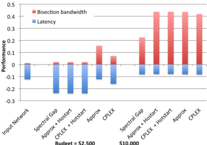
fat--‐0.2 -‐0.1 0 0.1 0.2 0.3 0.4 0.5 Input Fat-‐tr ee Greed y REW IRE Fat-‐tr ee Greed y REW IRE Fat-‐tr ee Greed y REW IRE Fat-‐tr ee Greed y REW IRE Pe rf or m an ce Bisec=on bandwidth Latency Budget = $1,250 $2,500 $5,000 $10,000 Fig. 2: Results of upgrading the SCS topology with different budgets and algorithms. -‐0.3 -‐0.2 -‐0.1 0 0.1 0.2 0.3 0.4 0.5 Input Netw ork Spec tral Gap Appro x + Ho start CPLE X + Ho tstart Appro x CPLE X Spec tral Gap Appro x + Ho start CPLE X + Ho tstart Appro x CPLE X Pe rf or m an ce Budget = $2,500 $10,000 BisecFon bandwidth Latency
Fig. 3: Results of upgrading the SCS topology with different REWIRE modes and two budgets.
tree constructed with the same budget, and with budgets over $5K, REWIRE’s network also has a shorter diameter (by 1 hop) than a fat-tree. REWIRE also outperforms the greedy algorithm for all budgets, though it does perform nearly as well as REWIRE when the budget is $5K or more. This indicates that a greedy approach performs very well in some settings; however, we have generally observed that the greedy algorithm does not perform well when it has a small budget or a very constrained input where few ports are open. As an example, when the budget is $2,500, REWIRE’s network has 350% more bisection bandwidth than the network found by the greedy algorithm.
Next, we compared the various modes of REWIRE for two budgets as shown in Figure3. We observe that the spectral gap and hotstart modes performs poorly when the budget is $2,500. This is likely due to the properties of the spectral gap, which tries to make the network more regular. Because the budget is not large enough to re-wire the network in this regular fasion, optimizing the network’s spectral gap creates a candidate solution with poor bisection bandwidth. This problem does not arise when the budget is large enough (as in the case when the budget is $10K), because there is enough money to re-wire
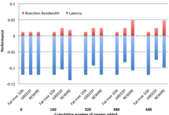
-‐0.15 -‐0.1 -‐0.05 0 0.05 0.1 Fat-‐tr ee 1G b GREED Y REW IRE Fat-‐tr ee 1G b GREED Y REW IRE Fat-‐tr ee 1G b GREED Y REW IRE Fat-‐tr ee 1G b GREED Y REW IRE Fat-‐tr ee 1G b GREED Y REW IRE Pe rf or m an ce
Bisec8on Bandwidth Latency
0 160 320 480 640 Cumula5ve number of servers added
Fig. 4: Results of iteratively expanding the SCS data center.
-‐0.2 -‐0.1 0 0.1 0.2 0.3 0.4 Fat-‐tr ee 1G b Fat-‐tr ee 10 Gb REW IRE Fat-‐tr ee 1G b Fat-‐tr ee 10 Gb REW IRE Fat-‐tr ee 1G b Fat-‐tr ee 10 Gb REW IRE Fat-‐tr ee 1G b Fat-‐tr ee 10 Gb REW IRE Fat-‐tr ee 1G b Fat-‐tr ee 10 Gb REW IRE Pe rf or m an ce Bisec8on Bandwidth Latency 0 160 320 480 640
Cumula5ve number of servers added
Fig. 5: Results of iteratively expanding a greenfield network.
the network into this regular structure. E. Expanding
We now examine the performance of the algorithms as we expand the data center over time by incrementally adding new servers. We tested two expansion scenarios here.
First, we expanded the SCS data center by adding 160 servers at a time, until we have added a total of 640 servers to the data center. The results are shown in Figure 4. For REWIRE and the greedy algorithm, we used ToR switches with 48 1Gbps and 4 10Gbps ports, so each ToR attaches to 40 servers. For the 1Gb fat-tree, we used ToR switches with 24 1Gbps ports. The budgets shown in the figure are the cabling budgets given to REWIRE; not the total budget that includes switches.
We found that REWIRE outperforms the fat-tree and the greedy algorithm in this scenario. The fat-tree is not able to improve the bisection bandwidth of the expanded network beyond the bisection bandwidth of the initial SCS DCN, whereas both the greedy algorithm and REWIRE do, while also decreasing the network latency. This scenario shows the limitations of the greedy algorithm. After four expansion iter-ations, REWIRE’s network has nearly twice as much bisection bandwidth as the greedy algorithm’s network.
Next, we expanded a greenfield data center using the two approaches. In these experiments, we built the initial DCN with a budget of $40K using REWIRE or a fat-tree with 1 or 10Gb links. This initial data center contained 1600 servers.
Then, we iteratively expanded this data center by adding 4000 servers at a time. For each expansion, the algorithms were given a total budget of $60K (this includes the cost of ToR switches). The results are shown in Figure 5.
Again, REWIRE performed better than either fat-tree con-figuration.
F. Quantitative results
We now evaluate the speedup we gain by utilizing the GPU to for our all-pairs shortest-path (APSP) solver implementa-tion. Our approximation algorithm to compute a network’s bisection bandwidth needs to solve hundreds of APSP prob-lems, and this computation is the bottleneck in its operation. Therefore, if we can solve APSP twice as fast, then it will take nearly half as much time to run REWIRE.
The following table shows the speedup achieved by our GPU implementation of APSP versus a high-performance CPU implementation [25] and the naive implementation de-scribed in [13].
n GPU runtime SPIRAL speedup CLRS speedup
64 0.092 0.211 2 2.66 28
128 0.274 1.5 5 20.31 74
256 0.733 9.83 13 112.8 153
512 3.435 51.6 15 839.63 244
1024 17.988 419 23 6020 334
TABLE IV: Comparison of our GPU implementation on NVIDIA Tesla C2050 with the CPU running times reported in [25] using the SPIRAL program generator and our implementation of APSP following the description in [13]. The reported times for SPIRAL use an auto-tuned 4-way vectorization of the Floyd-Warshall algorithm on Pentium 4.
V. OPERATING AN ARBITRARYDCN
In this paper, we have advocated for the adoption of non-regular topologies in the data center. Doing so raises architecture issues. In particular, we need to be able to provide addressing, routing, load-balancing and cost-effective management on arbitrary DCN topologies if they are to be of practical use. We now show how previous work can perform these functions.
Addressing and routing: have been the focus of much recent work due to the difficulty of scaling traditional, dis-tributed control-plane protocols to connect more than a couple thousand servers. VL2 [20] and PortLand [40] are scalable L2 networking architectures designed specifically for data center environments. Both proposals can scale to hundreds of thousands of end-hosts; however, they only work on networks with a Clos topology. Protocols such as SEATTLE [33] and TRILL [50] provide scalable L2 functionality on arbitrary topologies, but do not provide multipath routing, which is needed to fully utilize dense networks.
However, we can get scalable L2 networking and multipath routing by using SPAIN [38]. SPAIN uses commodity switches and servers. It modifies end-hosts and uses VLANs to partition the network into path-disjoint subgraphs.
Load-balancing: we assume that a network’s bandwidth can be fully exploited by the load-balancing mechanism. This assumption is not valid when using single-path protocols like
spanning tree; however, near-optimal load-balancing can be achieved on arbitrary topologies by using Multipath TCP [46] or SPAIN [38]. Centralized flow controllers like Hedera [2] and Mahout [15] could also be modified to provide near-optimal load-balancing.
Multipath TCP exposes multiple to-end paths to end-hosts, and they independently attempt to maximize their bandwidth by performing adaptive load balancing across these paths. This approach can achieve 100% utilization on a fat-tree [46]. Multipath TCP has not yet been evaluated on arbitrary topologies; however, its performance on regular topologies indicates it will be able to fully utilize arbitrary topologies as well.
SPAIN [38] performs reactive load balancing at the end-hosts over the various VLANs exposed to each end-host. It has been shown that SPAIN can fully utilize HyperX, FatTree and BCube topologies. Because it performs well on this range of regular topologies, we believe it will also perform well on the topologies REWIRE designs.
Management and configuration:managing an DCN with an irregular topology may be more costly and require more expertise than a vendor-specified DCN architecture. In par-ticular, addressing is more difficult to configure an irregular topology, because we cannot encode topologic locality in the logical ID of a switch (typically a switch’s logical ID is its topology-imposed address or label). However, such a network can be configured using Chen et al.’s generic and automatic data center address configuration system (DAC) [9]. DAC automates the assignment of logical IDs (e.g., IP addresses or node labels) to network devices. DAC begins with a network blueprint which specifies the logical ID, and then automatically learns devices IDs (e.g., MAC addresses). An interesting benefit of DAC’s design is that it can automatically identify mis-wirings. This operation is especially useful for us because wiring an arbitrary topology may be more difficult than a regular, tree-like topology. We believe DAC can solve many of the management problems that may arise from the introduction of irregular topologies in the data center, and we leave further investigation to future work.
VI. DISCUSSION
The (1 +)-approximation algorithm we implemented to compute the bisection bandwidth of a network is numerically unstable. At each iteration of its operation, it performs an all-pairs shortest-path computation. To do this, it needs to com-pare increasingly minute numbers at each successive iteration. We found it returns incorrect shortest-paths trees after enough iterations because these comparisons are made on numbers less than 10−40. Because of this numerical instability, we could
not run the approximation algorithm on inputs larger than 200 nodes and 200 edges. Nor could we run it with very small values ofbecause the algorithm performs more iterations as
decreases.
We believe it would be interesting to incorporate output topology constraints into REWIRE’s algorithm. This would allow users to constrain REWIRE’s output to a family of
topology constructions (e.g., Clos, fat-tree, BCube or HyperX). Doing so would generalize algorithms of Mudigonda et al. [39], who proposed algorithms to find min-cost constructions for fat-trees and HyperX networks.
We did not explicitly consider designing upgrades or ex-pansions that can be executed with minimal disruption to an existing DCN. However, it is possible to disable REWIRE’s support for moving existing network links. The greedy algo-rithm we compared REWIRE against never moves existing links, so we believe its results are indicative of the results such a modification to REWIRE would have. Another approach is to modify the cost constraints (e.g., moving a link costs five times more than adding a new one) so that rare, significantly beneficial re-wirings are permissible.
VII. CONCLUSIONS
In this paper, we proposed REWIRE, a framework to design data center networks. REWIRE uses local search to find a network that maximizes bisection bandwidth while minimizing latency and satisfying a large number of user-defined con-straints. REWIRE’s network design algorithm finds networks that significantly outperform networks found by other pro-posals. This optimization-based approach is flexible—it can design greenfield networks and upgrades or expansions of existing networks—and effective. For example, REWIRE finds greenfield networks with over 500% more bisection bandwidth and less worst-case end-to-end latency than a fat-tree built with the same budget.
To achieve these results, REWIRE builds arbitrary net-works, rather than the topology-constrained networks most existing data center use. REWIRE demonstrates that arbitrary topologies can boost DCN performance while reducing net-work equipment expenditure. Traditionally DCN design has restricted the topology to only a few classes of topologies, because it is difficult to operate an arbitrary topology in a high-performance environment. These difficulties have been mitagated by recent work [38], [9], so it may be time to move away from highly regular DCN topologies because of the performance benefits arbitrary topologies offer.
APPENDIXA
In this appendix, we sketch our GPU-based implementation of a all-pairs shortest-path (APSP) solver. GPUs are powerful and affordable, though have been traditionally difficult to program. However, new general purpose GPU (GPGPU) pro-gramming frameworks such as CUDA and OpenCL [42], [32] allow programmers to easily use the computational power of GPUs. Modern GPUs are equipped with hundreds of cores and are inexpensive; for example, NVIDIA introduced GeForce GTX 560 Ti in 2011 which has 384 cores offering 1.2 teraflops of computing power for $250 [43].
CUDA [42] extends the C++ language with parallel primi-tives and an extensive API for exposing the parallel features of the GPU. CUDA allows the programmer to group a large number of threads into thread blocks. A blocks is a group of single instruction multiple data (SIMD) threads. GPUs exhibit
a high memory bandwidth, and a high latency per memory access, though this can usually be compensated by clever scheduling of memory access requests, and careful reordering of the program logic so that memory access can be hidden.
We implemented a recursive version of the Floyd-Warshall algorithm for our APSP function using CUDA [8]. The algorithm uses generalized matrix multiplication (GEMM) as an underlying primitive. GEMM exhibits a high degree of data parallelism and we can significant speedups by exploiting this attribute. Finally, we perform a parallel reduction to find the maximal path in the distance matrix. Parallel reduction is an efficient algorithm for computing associative operators in parallel. It uses Θ(n) threads to compute a tree of partial results in parallel. The number of steps is bounded by the depth of the tree which is Θ(logn)[28], [26].
REFERENCES
[1] J. H. Ahn, N. Binkert, A. Davis, M. McLaren, and R. S. Schreiber. Hy-perx: topology, routing, and packaging of efficient large-scale networks. In Proceedings of the Conference on High Performance Computing Networking, Storage and Analysis (SC ’09), 2009.
[2] M. Al-Fares, S. Radhakrishnan, B. Raghavan, N. Huang, and A. Vahdat. Hedera: Dynamic Flow Scheduling for Data Center Networks. InNSDI, 2010.
[3] M. Alizadeh, A. Greenberg, D. A. Maltz, J. Padhye, P. Patel, B. Prab-hakar, S. Sengupta, and M. Sridharan. Dctcp: Efficient packet transport for the commoditized data center. InSIGCOMM, 2010.
[4] V. E. Beneˇs. Mathematical Theory of Connecting Networks and Telephone Traffics. Academic Press, 1965.
[5] T. Benson, A. Akella, and D. Maltz. Network traffic characteristics of data centers in the wild. InIMC, 2010.
[6] T. Benson, A. Anand, A. Akella, and M. Zhang. Understanding data center traffic characteristics. InProceedings of the 1st ACM workshop on Research on enterprise networking (WREN), 2009.
[7] D. Bertsimas and J. Tsitsiklis. Simulated annealing.Statistical Science, 8(1):10–15, 1993.
[8] A. Buluc¸, J. R. Gilbert, and C. Budak. Solving path problems on the gpu.Parallel Comput., 36:241–253, June 2010.
[9] K. Chen, C. Guo, H. Wu, J. Yuan, Z. Feng, Y. Chen, S. Lu, and W. Wu. Generic and automatic address configuration for data center networks. InSIGCOMM, pages 39–50, New York, NY, USA, 2010. ACM. [10] F. R. K. Chung. Spectral Graph Theory. 1994.
[11] Cisco. Cisco data center network architecture and solutions overview. White paper, 2006. Available online (19 pages).
[12] C. Clos. A study of non-blocking switching networks. Bell System Technical Journal, 32(5):406–424, 1953.
[13] T. H. Cormen, C. E. Leiserson, R. L. Rivest, and C. Stein. Introduction to Algorithms. The MIT Press, 3rd edition, 2009.
[14] A. R. Curtis, S. Keshav, and A. L´opez-Ortiz. LEGUP: Using hetero-geneity to reduce the cost of data center network upgrades. InCoNEXT, 2010.
[15] A. R. Curtis, W. Kim, and P. Yalagandula. Mahout: Low-overhead datacenter traffic management using end-host-based elephant detection. InINFOCOM, 2011.
[16] A. R. Curtis and A. L´opez-Ortiz. Capacity provisioning a valiant load-balanced network. InINFOCOM, 2009.
[17] Digital Reality Trust. what is driving the US market? White paper, 2011. Available online athttp://knowledge.digitalrealtytrust.com/.
[18] L. Donetti, F. Neri, and M. A. Munoz. Optimal network topologies: Expanders, cages, ramanujan graphs, entangled networks and all that. Journal of Statistical Mechanics: Theory and Experiment, 8, 2006. [19] EPA. EPA report to congress on server and data center energy efficiency.
Technical report, U.S. Environmental Protection Agency, 2007. [20] A. Greenberg, J. R. Hamilton, N. Jain, S. Kandula, C. K. P. Lahiri,
D. Maltz, P. Patel, and S. Sengupta. VL2: a scalable and flexible data center network. InSIGCOMM, 2009.
[21] A. G. Greenberg, J. R. Hamilton, D. A. Maltz, and P. Patel. The cost of a cloud: research problems in data center networks. Computer Communication Review, 39(1):68–73, 2009.
[22] C. Guo, G. Lu, D. Li, H. Wu, X. Zhang, Y. Shi, C. Tian, Y. Zhang, and S. Lu. BCube: a high performance, server-centric network architecture for modular data centers. InSIGCOMM, 2009.
[23] C. Guo, H. Wu, K. Tan, L. Shi, Y. Zhang, and S. Lu. Dcell: a scalable and fault-tolerant network structure for data centers. In SIGCOMM, 2008.
[24] J. R. Hamilton. Data center networks are in my way. Presented at the Standford Clean Slate CTO Summit, 2009.
[25] S.-C. Han, F. Franchetti, and M. P¨uschel. Program generation for the all-pairs shortest path problem. InParallel Architectures and Compilation Techniques (PACT), pages 222–232, 2006.
[26] W. D. Hillis and G. L. Steele, Jr. Data parallel algorithms. Commun. ACM, 29:1170–1183, December 1986.
[27] U. Hoelzle and L. A. Barroso. The Datacenter as a Computer: An Introduction to the Design of Warehouse-Scale Machines. Morgan and Claypool Publishers, 2009.
[28] D. Horn. Stream Reduction Operations for GPGPU Applications, volume 2, chapter 36. 2005.
[29] IBM. IBM ILOG CPLEX Optimizer.http://www-01.ibm.com/software/ integration/optimization/cplex-optimizer/.
[30] M. Isard, M. Budiu, Y. Yu, A. Birrell, and D. Fetterly. Dryad: distributed data-parallel programs from sequential building blocks. In EuroSys, 2007.
[31] S. Kandula, S. Sengupta, A. Greenberg, and P. Patel. The nature of datacenter traffic: Measurements & analysis. InIMC, 2009.
[32] Khronos OpenCL Working Group. The opencl specification, version 1.0.29, 8 December 2008.
[33] C. Kim, M. Caesar, and J. Rexford. Floodless in seattle: a scalable ethernet architecture for large enterprises. InSIGCOMM, 2008. [34] J. Kim, W. J. Dally, and D. Abts. Flattened butterfly: a cost-efficient
topology for high-radix networks. SIGARCH Comput. Archit. News, 35(2), 2007.
[35] S. Kirkpatrick, C. D. Gelatt, and M. P. Vecchi. Optimization by simulated annealing. Science, 220(4598):671–680, 1983.
[36] M. Kodialam, T. V. Lakshman, J. B. Orlin, and S. Sengupta. Oblivious routing of highly variable traffic in service overlays and ip backbones. IEEE/ACM Trans. Netw., 17:459–472, April 2009.
[37] C. E. Leiserson. Fat-trees: universal networks for hardware-efficient supercomputing. IEEE Trans. Comput., 34(10):892–901, 1985. [38] J. Mudigonda, P. Yalagandula, M. Al-Fares, and J. C. Mogul. SPAIN:
COTS data-center ethernet for multipathing over arbitrary topologies. In NSDI, 2010.
[39] J. Mudigonda, P. Yalagandula, and J. C. Mogul. Taming the flying cable monster: A topology design and optimization framework for data-center networks. InUSENIX ATC, 2011.
[40] R. N. Mysore, A. Pamboris, N. Farrington, N. Huang, P. Miri, S. Rad-hakrishnan, and V. Subram. Portland: A scalable fault-tolerant layer 2 data center network fabric. InSIGCOMM, 2009.
[41] Y. Nourani and B. Andresen. A comparison of simulated annealing cooling strategies. Journal of Physics A: Mathematical and General, pages 8373–8385, 1998.
[42] NVIDIA. NVIDIA CUDA. http://www.nvidia.com/object/cuda home new.html.
[43] NVIDIA Corporation. GeForce GTX 560 Ti. http://www.nvidia.com/ object/product-geforce-gtx-560ti-us.html. Accessed: 07/25/2011. [44] Y. Peres, D. Sotnikov, B. Sudakov, and U. Zwick. All-pairs shortest
paths ino(n2)time with high probability. InFOCS ’10, 2010.
[45] L. Popa, S. Ratnasamy, G. Iannaccone, A. Krishnamurthy, and I. Stoica. A cost comparison of data center network architectures. InCoNEXT, 2010.
[46] C. Raiciu, S. Barre, C. Pluntke, A. Greenhalgh, D. Wischik, and M. Handley. Improving datacenter performance and robustness with multipath tcp. InSIGCOMM, 2011.
[47] M. R. Samatham and D. K. Pradhan. The de bruijn multiprocessor network: A versatile parallel processing and sorting network for vlsi. IEEE Trans. Comput., 38:567–581, April 1989.
[48] A. Singla, C.-Y. Hong, L. Popa, and P. B. Godfrey. Jellyfish: Networking data centers randomly. InHotCloud, June 2011.
[49] H. Tangmunarunkit, R. Govindan, S. Jamin, S. Shenker, and W. Will-inger. Network topology generators: degree-based vs. structural. In SIGCOMM, 2002.
[50] J. Touch and R. Perlman. Transparent Interconnection of Lots of Links (TRILL): Problem and Applicability Statement. RFC 5556 (Informational), May 2009.
[51] A. Vierra. Case study: NetRiver rethinks data center infrastructure design. Focus Magazine, August 2010. Available online at http: //bit.ly/oS4pCu.
[52] H. Wu, G. Lu, D. Li, C. Guo, and Y. Zhang. MDCube: a high performance network structure for modular data center interconnection. InCoNEXT, 2009.
[53] A. Y. Zomaya and R. Kazman. Algorithms and theory of computation handbook. chapter Simulated annealing techniques, pages 33–33. Chapman & Hall/CRC, 2010.